Revisiting Forest Effects on Winter Air Temperature and Wind Speed—New Open Data and Transfer Functions

Abstract

The diurnal cycle of both air temperature and wind speed is characterized by considerable differences, when comparing open site conditions to forests. In the course of this article, a new two-hourly, open-source dataset, covering a high spatial and temporal variability, is presented and analyzed. It contains air temperature measurements (128 station pairs (open/forest); six winter seasons; six study sites), wind speed measurements (64 station pairs; three winter seasons, four study sites) and related metadata in central Europe. Daily cycles of air temperature and wind speed, as well as further dependencies of the effective Leaf Area Index (effective LAI), the exposure in the context of forest effects, and the distance to the forest edge, are illustrated in this paper. The forest effects on air temperature can be seen particularly with increasing canopy density, in southern exposures, and in the late winter season, while wind speed depends on multiple factors such as effective LAI or the distance to the forest edge. New transfer functions, developed using linear and non-linear regression analysis, in a leave-one-out cross-validation, improve certain efficiency criteria (NSME; r²; RMSE; MAE) compared to existing transfer functions. The dataset enables multiple purposes and capabilities due to its diversity and sample size.

1. Introduction

The climate in the boundary layer and, thus, the micrometeorological variables are strongly dependent on the nature of the environment, which enables understanding air temperature and wind speed profiles by considering their surrounding area [1].

As a rule, in the boundary layer, air temperature in the open field decreases with altitude during the day and increases with altitude at night (nocturnal inversion). The reason behind this phenomenon is the ground’s heat absorption during the day, which depends on the albedo value and radiation, and its emission at night through long-wave radiation [1] and downhill katabatic wind. In the forest, this diurnal cycle of air temperature differs from open site conditions. The maximum air temperature during the day is lower due to radiation shading by the canopy [2]. Below the tree canopy, the temperature profile is consequently characterized by a lower amplitude [1].

Regarding wind speed, forests generate higher turbulence compared to other surfaces, due to their roughness [1]. Thus, the impact of the canopy on microclimate below is particularly high in regards to wind speed. The active surface of the energy balance in the open field influences the micrometeorology in the boundary layer. Forests increase the active surface in terms of vertical distance from the forest ground to the canopy section with highest leaf density. Above the trees, wind speed increases logarithmically and from the top of the trees to the active surface it decreases sharply [1]. Slightly below, the wind speed is most attenuated by the large aerodynamic resistance. Beneath the canopy, a mini-jet arises (i.e., a shallow layer with a local maximum of wind speed) and on ground the wind speed becomes zero [1]. This slightly greater airflow below the canopy causes the air to be mixed and the air temperature gradient between the ground and the canopy is low [3]. The size of clearings [4] and wind speed [5] play a role in the question whether wind can form in gaps in the forest or whether the forest cover is considered closed. Wind speed in the open field is, thus, typically greater than in the forest, but above the forest, the turbulence in the atmosphere extends to higher layers [1]. Wind speed depends largely on the type of forest, but slope orientation, topography, and the stability of the air layers also have an influence [3]. In general, it can be said that because of the increased active surface, the daily maximum air temperature and wind speed are lower in the forest than in the open field [6,7,8].

Understanding climatic effects between forested and open areas is important to, for example, accurately simulate snow processes or eco-hydrological mechanisms in forested environments. Snow models require micrometeorological values from the forest for calculating hydrological processes such as snowmelt or snow distribution [9,10]. Typically, meteorological measurements are collected at open field sites [11] and not within forests.

This article can make a contribution to comprehending the interactions between open field and forest sites, regarding winter micrometeorology. Forest characteristics can, for example, be described by its leaf area index (LAI) [12]. Such a parameter enables calculations of climatic differences between forest and open field with transfer functions that use forest parameters and meteorological variables. Examples in snow hydrology, among others, are “SNOWMODEL” [13], “AMUNDSEN” [14], “ESCIMO” [15], and “WaSiM” [11]. Recent publications have increasingly focused on the influence of the canopy on wind speed and radiation, and consequently air temperature, and assign an important role to these factors for snow distribution and snowmelt [9,10]. Due to variations in snow accumulation in forests and canopies, extensive datasets are crucial for empirical model development [16]. The temporal resolution of meteorological data also plays an important role for snowpack models. According to [17], significant underestimations of snow water equivalent (SWE) and melt rate occur at time steps larger than one hour because the precipitation phase is poorly represented. Larger time steps might cause an increase in errors between observation and simulation. It is also confirmed that in areas with a lot of snow, three-hourly time intervals can be sufficient for good model results [18].

This publication presents a comprehensive dataset of two-hourly measurements of air temperature and wind speed at forest stations and neighboring stations in the open field, collected during different winter seasons and study sites in central Europe. In addition, characteristics of the study areas and forest parameters are compiled. The dataset’s visualization presented here, as well as the development of new transfer functions, might be an inspiration for its usage. Especially its advantages of sample size and spatial diversity can offer benefits in the development of new models or testing hypotheses.

2. Materials and Methods

2.1. Study Sites and Observation Network

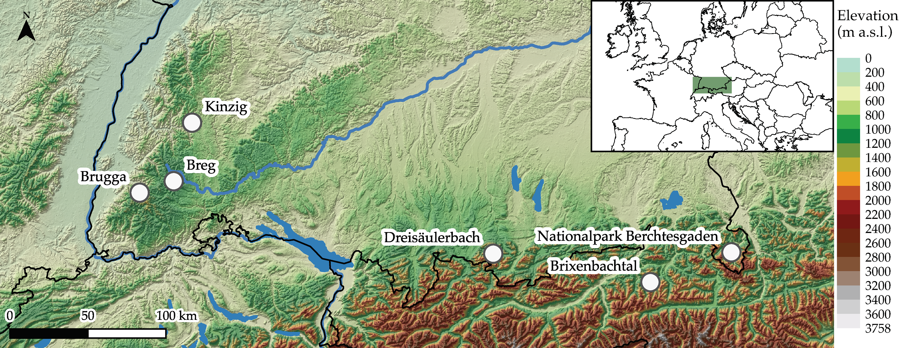
The research areas used for data collection are located in southern Germany (Black Forest and Bavarian Alps) and the Austrian Alps (Brixenbachtal) (see Figure 1).

Black Forest: The Black Forest is a typical midlatitude medium elevation mountain range in the southwest of Germany. Three study catchments, Kinzig (KIN), Breg (BRE), and Brugga (BRU), were equipped with observation stations. The mountain range has elevations ranging from approximately 400–1493 m a.s.l. Average winter season air temperatures range from 4.1 °C in the lower parts to −2.1 °C in the highest elevations. Mean annual precipitation ranges from approximately 900 mm in the lower parts to about 1950 mm in the higher regions. More than half of precipitation falls during the winter months. Prevailing main wind direction in the area is westerly. On average, only 3% of the study catchment areas are covered by human settlements while 27% are open areas, used for grazing and haymaking. The remaining 70% of the area is covered by forest. The forests in the Black Forest are about 80% coniferous (spruce, fir, pine) and 20% deciduous (beech, birch, oak). The most common needle leaf species is the European spruce (Picea abies), while the most common deciduous tree species is beech (Fagus sylvatica).

Nationalpark Berchtesgaden (NPB): This study area is located in the Berchtesgaden Alps of southeastern Germany and is part of the Berchtesgaden National Park. The National Park comprises an area of 210 km². The region is characterized by an extreme topography with mountain ranges covering an altitude from 603 to 2713 m a.s.l. Due to its status as a biosphere reserve, land use primarily depends on environmental protection policies and is only marginally influenced by economic activities. The main ecosystem types found in the catchment are forest (47.7%), rock and rubble fields (25.3%), grass covered communities (13,7%), mountain pine and green alder shrubs (7.2%) as well as lakes (1.7%). The main soil types in the region are Syrosem (35.5%), Cambisol (30.1%), and Podsol (26.7%).

Dreisäulerbach (DSB): This study catchment is located in the Ammergauer Alps of southern Germany. The Ammergauer Alps can be considered a typical subalpine mountain range. The catchment ranges from 940 m a.s.l. to over 1700 m a.s.l. and covers an area of about 2.6 km². The bedrock within the catchment is mainly made up of Cenoman-Turon and local limestone (Wettersteinkalk). In the higher regions, considerable areas are covered with slope weathered rock. The soil layer catchment consists mainly of cambisol and rendzina. Other soil types only occur in minor proportions. The surface, especially in the lower regions, is predominantly covered with coniferous forests. In the upper, steeper, regions of the catchment, significant patches of grassland can be found. The mean annual precipitation is about 1757 mm. The monthly average temperature varies from −1.5 °C in January to 16.1 °C in July.

Brixenbachtal (BRX): The Brixenbach valley is a small subalpine catchment situated in the Kitzbühel Alps in Northern Tyrol, Austria. The size of the Brixenbach catchment is 9.3 km², with a mean elevation of 1370 m a.s.l. The highest point (Gampenkogel) has an elevation of 1956 m a.s.l. and the discharge gauge of the Hydrographic Service of Tyrol (installed in 2004) at the catchment outlet is at 818 m a.s.l. The mean annual precipitation sum at the precipitation gauge at Nachtsöllberg (990 m a.s.l.), close to the catchment outlet, is about 1400 mm, and the mean duration of snow cover amounts to 132 days (1990–2010, Hydrographic Service of Tyrol). The bedrock belongs to the Paleozoic Greywacke zone and is, thus, dominated by porphyroids and shales (slightly metamorphic sand-, siltand claystones), partly overlain by Mesozoic dolomites. Mostly shallow cambisols, podsols, partly gleysols and—in the dolomite areas—rendzinas have developed on the Quarternary sediment coverage (moraines, talus deposits, colluvium). The catchment area is mainly covered by oligotrophic cattle pastures (44%) and forests (35%). Rock faces and talus slopes cover 14% of the catchment, and only small areas are used as hay meadows for settlements, ski-slopes, and forest road. The forests are dominated by conifers, with spruce (Picea abies) being the predominant tree species. Larch trees (Larix), firs (Abies), mountain pines (Pinus mugo), Swiss stone pines (P. cembra), grey and green alders (Alnus incana, A. viridis) occur in smaller proportions.

Networks consisting of different numbers of microclimatic measurement stations were established during different winter seasons in the study areas (see

Table 1. Number of measurement stations separated by study area, year, and micrometeorological quantity.

Study Area	2012	2013	2014	2015	2016	2017
Brugga (BRU)	- -	TEMP (5) -	TEMP (14) -	TEMP (5) WIND (5)	- -	- -
Breg (BRE)	TEMP (7) -	TEMP (9) -	TEMP (8) -	- -	- -	- -
Kinzig (KIN)	TEMP (9) -	TEMP (10) -	- -	- -	- -	- -
Dreisäulerbach (DSB)	- -	- -	- -	- -	TEMP (7) WIND (7)	TEMP (3) WIND (3)
Brixenbachtal (BRX)	- -	- -	- -	TEMP (3) WIND (3)	- -	- -
Nationalpark Berchtesgaden (NPB)	- -	- -	- -	TEMP (8) WIND (7)	TEMP (26) WIND (25)	TEMP (14) WIND (14)

). The snow monitoring station (SnoMoS) is a standalone measurement system able to measure snow depth, air temperature, relative humidity, incoming shortwave radiation, surface temperature, barometric pressure, and wind speed/precipitation. A comprehensive description of the SnoMoS can be found in [19]. A stratified sampling design was used to cover a wide range of elevations and exposures within the study areas. To specifically investigate the influence of the vegetation cover, pairs of SnoMoS were generally installed in close proximity to each other, with one being located underneath the canopy while the other was situated on an adjacent open field site. In this study, only measurements of air temperature and wind speed are presented, since those are the variables with the most measurements available in total.

2.2. Dataset

The presented dataset consists of time series of two-hourly measurements of air temperature and wind speed. The data was initially collected to study the spatio-temporal variability of micrometeorological variables describing the energy balance of the snowpack [19]. The micrometeorological data is listed in station pairs of neighboring stations. Metadata for each location and station pair, respectively, are also part of the dataset. The available parameters are summarized below in

Table 2. Parameters of the metadata with the respective unit and a short explanation.

Parameter	Unit	Description
Pair_ID	(-)	Identification of the station pair
Location	(-)	Local description
Elevation_Open	(m a.s.l. )	Elevation open field
Elevation_Forest	(m a.s.l. )	Elevation forest
Exposure_Open	(°)	Exposure open field counterclockwise (0°/360° = north; 90° = west, etc.)
Exposure_Forest	(°)	Exposure forest counterclockwise (0°/360° = north; 90° = west, etc.)
Slope_Open	(°)	Slope open field
Slope_Forest	(°)	Slope forest
Effective_LAI	(m2m−2)	Effective leave area per ground area
Canopy_Openness	(%)	Openness of the canopy
Distance_Forest_Edge	(m)	Distance of the forest station to the closed forest edge
Distance_Open_Station	(m)	Distance between the paired stations

. The entire dataset is available for free and accessible (see Data availability section).

According to the two-hour intervals, there are 12 measurements per day. The air temperature (given in °C) and wind speed data (given in ms⁻¹) are structured in the same way and as follows: The time stamp (Date), the measurement in the open (Air_Temp_Open, Wind_Open), and the measurement in the forest (Air_Temp_Forest, Wind_Forest). The dataset consists of 128 station pairs with air temperature measurements and 64 station pairs with wind speed measurements (the total number of values amounts to 173 682 and 115 211, respectively). Near surface air temperature and wind speed are measured at 2 m above surface.

Elevation, slope, and exposure of the locations were derived from digital elevation models. Effective LAI and canopy openness was derived from hemispherical images. The distances were measured in the field or derived from georeferenced aerial images.

The used observation stations SnoMoS are additionally equipped with a photo diode that can be used to measure incoming global radiation. During days with high radiation inputs, distinct peaks of air temperature during noon were observed in the raw data of the measurements at the open field stations, which can be explained by radiative heating. A strong linear correlation between measured air temperature peaks and incoming radiation was observed and consequently used to correct the air temperature measurements for the solar heating bias at the open field stations. Due to the shading of forest trees such a bias was not observed at the forest stations and, thus, no correction of those measurements was conducted.

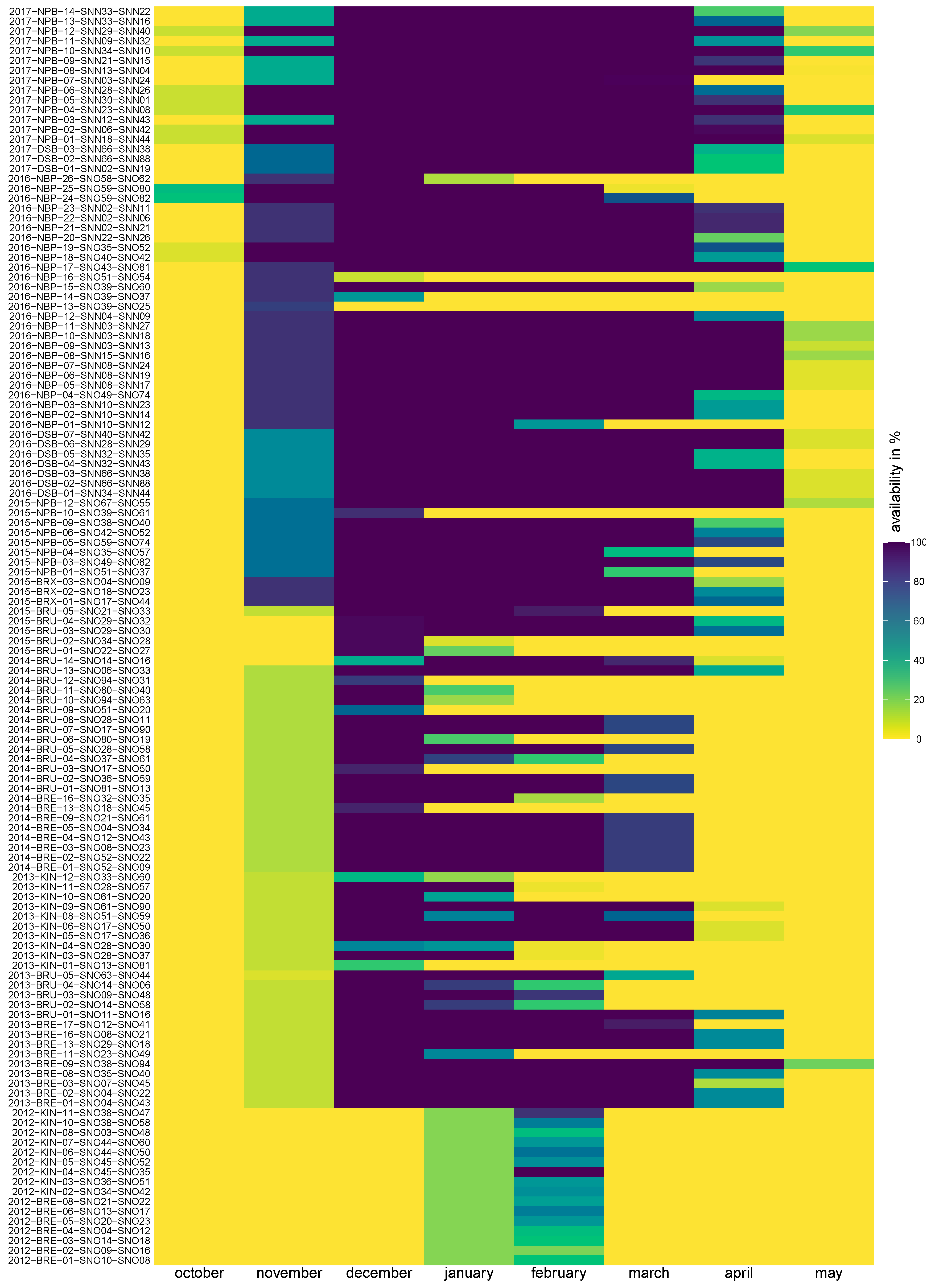
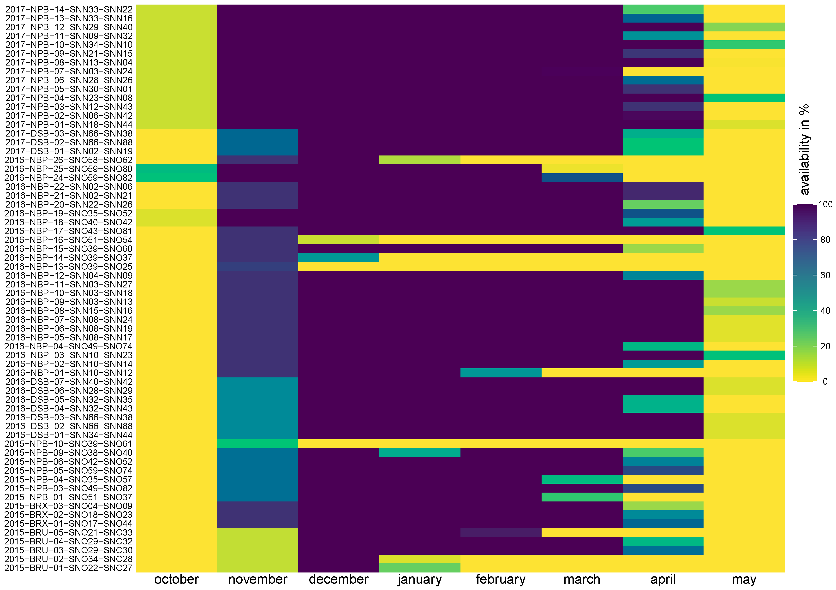
The measurements were recorded during six winter seasons. For each station pair, the available time period is shown in Appendix A for air temperature (Figure A1) and in Appendix A for wind speed (Figure A2), respectively.

The effective leaf area index (LAI) is the most important factor of the metadata because it summarizes the distribution of leaves, which has great influence on biological and physical processes in the forest and, thus, on micrometeorology [12]. The existing transfer functions apply the effective LAI [15], referring to the definition according to [12], which determines that tree trunks, branches, and leaves are included, but not aggregating effects, which describe that leaves are not randomly distributed and cover each other. The LAI value mentioned in this article and contained in the dataset adheres to this definition.

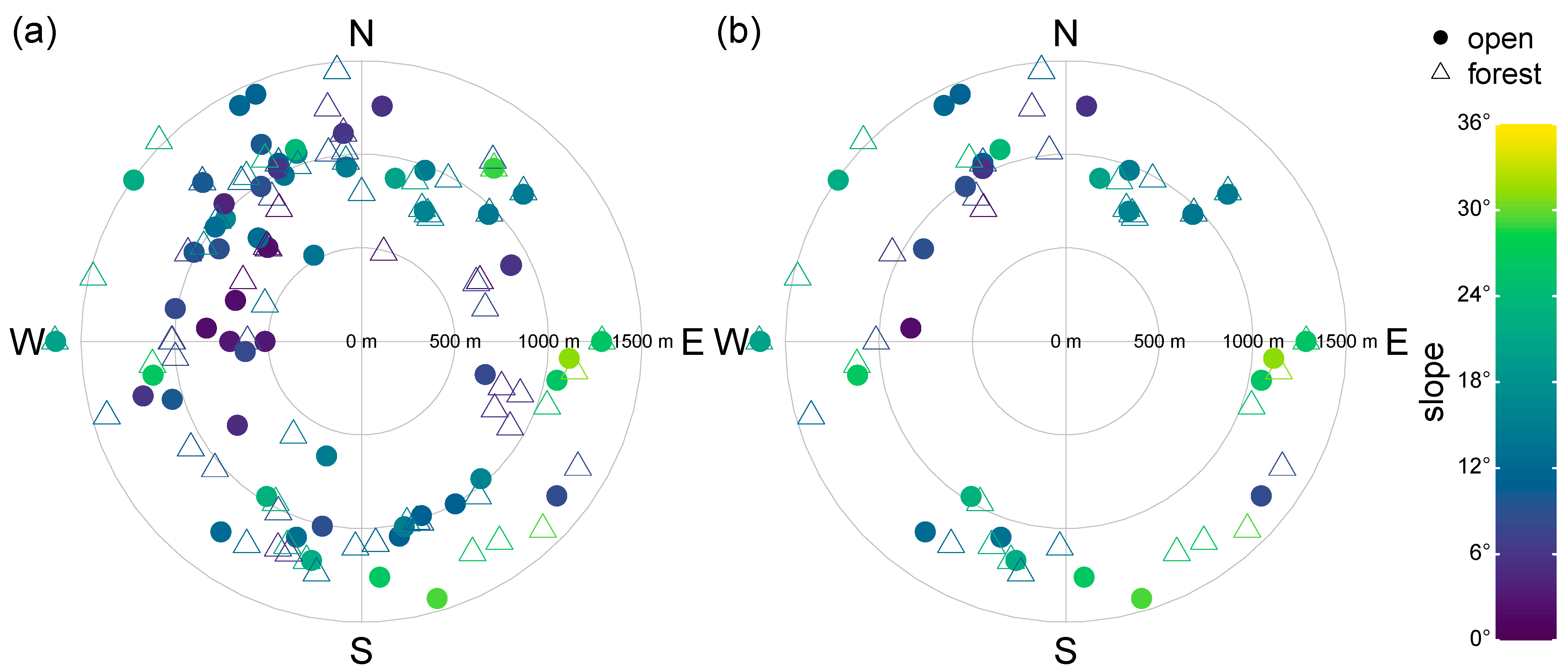
Figure 2 visualizes the range of terrain characteristics (i.e., slope and altitude) covered by the dataset. The 128 air temperature station pairs are comprised of 59 stations in the open field and 73 stations in the forest with different metadata. The 64 wind station pairs are comprised of 27 stations in the open field and 34 stations in the forest with different metadata.

2.3. Data Analysis

The dataset is used to elaborate forest effects and processes on winter air temperature and wind speed. In particular, their daily cycles as well as the interrelations between the metadata and the meteorological variables are considered. The dumping effects by the forest are explored with the effective LAI (air temperature) and the distance to the forest edge (wind speed). Furthermore, the impact of exposure on daily air temperature ranges are under examination. Finally, the dataset is used for evaluation of existing transfer functions and the development of new transfer functions.

2.4. Existing Transfer Functions

Empirical transfer functions for air temperature and wind speed are already available in the literature [11,13,14,15,20,21,22,23] and used in climate and snow models.

Refs. [11,13,14,15] follow the empirical approach of Obled [23] for calculating the air temperature in the forest based on the air temperature in the open field. The equation:

$$T_f=T_o-F_c\left\{T_o-\left[R_c\left(T_o-T_{mean}\right)+T_{mean}-\delta T\right]\right\}$$

(1)

expresses that the air temperature in the forest $T_f$ [K] can be calculated equal to the top-of-canopy air temperature $T_o$ [K] with an attenuation of the diurnal profile due to shading and nighttime thermal radiation emitted by the canopy. $R_c$ is a dimensionless scaling parameter (=0.8), $T_{mean}$ [K] is the mean daily air temperature in the open field and $\delta T$ [K] is a temperature offset based on $T_{mean}$ [20], as can be seen in Equation (2):

$$\delta T=\frac{\left(T_{mean}-273.16\right)}{3}.$$

(2)

The results of this formula were compared with meteorological values from Col de Porte (1420 m a.s.l.) in the French Alps and found to be good [20]. The condition −2 K $\le \delta T\le$ +2 K applies. $F_c$ (-) is a function, which expresses the canopy density depending on the effective leaf area index $LA{I}^{*}$ (m²m⁻²) with values between 0 and 1 and can be calculated by

$$F_c=a+b\times \ln \left(LA{I}^{*}\right),$$

(3)

where $a$ equals 0.55 (-) and $b$ equals 0.29 (-) following [24].

Three different approaches are mentioned for the calculation of wind speed. The variable $W_f$ (ms⁻¹) stands for wind speed in the forest and the variable $W_o$ (ms⁻¹) stands for wind speed in the open field. Hardy et al. [25] set up the equation:

$$W_f=max\left[\left(W_o\times 0.042\right)-0.04,0\right],$$

(4)

after a three-day measurement of wind speeds 2 m above the surface and above the canopy of a Banks pine forest. This formula is based on observations.

Link and Marks [26] have adopted a simple estimate by assuming the wind speed in the forest with 20% of the wind speed from the open field in Equation (5):

$$W_f=\frac{1}{5}\times W_o.$$

(5)

Liston and Elder [13], Strasser et al. [14], Marke et al. [15], and Förster et al. [11] follow a common approach, which is based on Cionco [22] and supplemented by Essery et al. [21]. It says that wind speed at the reference height in the forest can be calculated using the following equation:

$$W_f=W_o\times e^{-0.4\times f_i}.$$

(6)

The required canopy flux index f_i is determined using the Equation (7):

$$f_i=\beta \times LA{I}^{*},$$

(7)

where $\beta$ is a dimensionless scaling factor with the value 0.9, through which the effective leaf area index $LA{I}^{*}$ (m²m⁻²) is adjusted to be compatible with Cionco [13]. Marke et al. [15] follows this approach too, but has expressed it as follows:

$$W_f=W_o\times e^{-\alpha \times \left(\frac{1-z}{h}\right)},$$

(8)

$h$ (m) is the canopy height and $z$ (m) is the canopy reference level. The canopy flow index $\alpha$ (-) is calculated using $LA{I}^{*}$ (m²m⁻²) and the scaling factor $\beta$ = 0.9 (-):

$$\alpha =LA{I}^{*}\times \beta .$$

(9)

In addition, there are numerical and iterative approaches that iteratively calculate meteorological variables based on energy balances for each step and achieve good results [27,28]. However, there are also models that assume the values of the open field to be the values in the forest, if they are not available (e.g., SNTHERM) [25].

2.5. Developement of New Transfer Functions

For the development of new transfer functions, the differences and correlations between forest and open field are considered via literature and the observed data. In the event of recurring diurnal profiles, functions are extended to include factors that map these oscillations. Other factors that the functions contain are evaluated via simple and multiple linear regression analysis or non-linear regression. Care is taken to use as few parameters as possible in order to achieve good results for datasets with less information.

The linear least squares method is a common practice for regression analysis in geosciences [29], where the straight line between all pairs of values is determined with the observed and the calculated value, which produces the least sum of squared deviations to the values. The idea behind this is to create a linear combination of parameters that relate the values to each other. For more dynamical cases, the more complex, iterative non-linear least squares method is used, where initial values for the parameters sought must be estimated in advance [30]. Especially for wind speed, the non-linear method offers an approach for dampening large outliers.

2.5.1. Air Temperature

The air temperature in the forest is mostly within the daily range of the air temperature in the open field, thus, its profile is dampened. The transfer function according to Obled [23] (Equations (1) and (2)) and two new approaches are applied.

Approach T1 starts with a linear regression, which estimates the forest minimum and maximum daily air temperature depending on the open daily minimum and maximum air temperature via the variables $A$ and $B$. This regression results in following two equations for estimating the forest minimum and maximum based on every open field value:

$$T_{f,min,est}\left(t\right)=A_{min}\times T_o\left(t\right)+B_{min},$$

(10)

$$T_{f,max,est}\left(t\right)=A_{max}\times T_o\left(t\right)+B_{max}.$$

(11)

The maximum value is calculated under the assumption that the current air temperature [K] at time $t$ is the daily maximum value, while the minimum value is calculated under the assumption that the current air temperature is the daily minimum value. The range between $T_{f,min,est}\left(t\right)$ and $T_{f,max,est}\left(t\right),$ thus, gives the scope of the attenuation by determining the estimated air temperature between those values. The function for calculating the air temperature in the forest for every time step $T_f\left(t\right)$ [K]

$$T_f\left(t\right)=\left(\frac{T_o\left(t\right)-T_{o,daily,min}}{T_{o,daily,max}-T_{o,daily,min}}\right)\times \left(T_{f,max,est}\left(t\right)-T_{f,min,est}\left(t\right)\right)\times Fc+T_{f,min,est}\left(t\right),$$

(12)

reduces this estimation by the distance of the value in the open field at time $t$ from the daily minimum value. Due to the dumping effect of the forest on the air temperature, $T_{f,min,est}\left(t\right)$ must be higher than $T_o\left(t\right)$, respectively, $T_{f,min,est}\left(t\right)$ must be lower than $T_o\left(t\right)$. For this reason, the difference between $T_{f,max,est}\left(t\right)$ and $T_{f,min,est}\left(t\right)$ is negative and $T_{f,min,est}\left(t\right)$ (the last part of Equation (12)) is reduced. By multiplying with the factor $F_c$ (Equation (3)), the dampening of the air temperature is made dependent on the leaf area index. With an increasing $LA{I}^{*}$, the factor $F_c$ decreases and the forest’s dampening impact in this transfer function increases as well. $T_{o,daily,min}$ (K) stands for the daily minimum air temperature and $T_{o,daily,max}$ (K) stands for the daily maximum air temperature in the open field.

The second approach T2

$$T_f\left(t\right)=A\times F_c\times {\left(\left(\frac{T_o\left(t\right)-T_{o,daily,min}}{T_{o,daily,max}-T_{o,daily,min}}\right)-0.5\right)}^2\times \left(T_o\left(t\right)-T_{o,daily,mean}\right)+T_{o,daily,mean},$$

(13)

follows the idea that a quadratic equation at the beginning of the function determines the upward and downward deviation from the daily mean. The first part of the function works like a parabola, which operates with the comparison of the current air temperature and the respective daily mean. Low and high air temperatures, in the range of daily distribution, result in large numbers and for air temperatures close to the related daily mean, this part of the equation decreases towards zero. This factor is additionally made dependent on a scaling factor $A$ (-) and the factor $F_c$ (-). The second bracket of Equation (13) calculates the deviation of the daily mean and the air temperature in the open field at time $t$. Subsequently, this deviation is offset against the daily mean in the open field $T_{o,daily,mean}$ (K). The air temperature in the forest, thus, tends towards the mean value in the open field, whereby the amount of attenuation depends on the daily maximum and minimum values.

2.5.2. Wind Speed

The wind speed in the forest depends significantly on the wind speed above the forest and the structure of the trees. In the present dataset, however, the wind speed values in the open field do not come from above the canopy, which is why the assumption of a logarithmic wind profile does not necessarily work within the used measurement set-up (ground stations at open and forested sites). For this reason, approaches are pursued that assume linear proportions between the wind speed in the open field and the forest. The transfer functions according to Cionco [22] (Equation (6)) and Hardy et al. [25] (Equation (4)) are applied.

In addition, two further developments are considered. The first approach W1

$$W_f\left(t\right)=max\left(W_o{\left(t\right)}^A\times Fc-W_{o,mean}, 0\right)$$

(14)

takes up the function according to Hardy et al. [25]. $W_f\left(t\right)$ (ms⁻¹) and $W_o\left(t\right)$ (ms⁻¹) describe again wind speed in the forest and in the open field. $W_{o,mean}$ (ms⁻¹) stands for the average wind speed at the open station. In order to better represent higher wind speeds, the wind speed is quadratically adjusted with the dimensionless exponent $A$. In addition, the factor $F_c$ (-) is intended to represent the different densities of the foliage. Finally, this value is set in relation to the mean value at the respective station in the open field. The idea behind this is to receive a more specific function for the respective station pairs.

The second approach for wind speed W2

$$W_f\left(t\right)=max\left({\left(W_o\left(t\right)\times F_c\right)}^A-W_{o,mean},0\right)$$

(15)

is a further development of Equation (4). The underlying idea is including the factor $F_c$ (-) in the quadratic function to increase the forest effects due to exponent $A$ (-).

2.6. Leave-One-Out Cross-Validation & Efficiency Criteria

The new transfer function approaches are applied to the entire dataset by means of a cross-validation procedure and compared with the existing functions in order to proof and compare efficiency. More precisely, a repeated leave-one-out cross-validation (LOOCV) procedure is used because the dataset is limited [31]. In this procedure, parameter tuning is applied, utilizing a subset of the entire collection of values, in order to test the accuracy of the function—even for conditions not covered in the training dataset. Therefore, the predictive quality of the functions can be determined on new datasets [31]. The present dataset has many individual station pairs, which represent completed time series for different winter seasons. Here, each station pair becomes the test set once, while all other station pairs form the training set. Since not every measured value is omitted once, but always an entire pair of stations, this method is more like a k-fold cross-validation [32], with the difference that the omitted pairs of stations have different numbers of values. For the respective training set, the parameters of the respective function are calculated using mathematical methods. The function is then applied to the neglected station pairs and the efficiency criteria (see Sect. Appendix B) are determined and presented by violin plots in the results section. This aims to quantify their accuracy and to make the suitability of the transfer functions comparable. In addition to the boxplots, the violin plots show the probability density. Here, the width of the violins is normalized, so all violins have the same width at the position with the most values, and its respective scale. Therefore, the violins are not comparable among each other regarding width. Conclusions from the violin plots can be drawn by considering the density distribution for each violin. The coefficient of determination $r^2$, the Nash-Sutcliffe-Model Efficiency $NSME$, the Root Mean Square Error $RMSE$ and the Mean Average Error $MAE$ are used for the evaluation. The reason for multiple efficiency criteria lies in the different approaches as well as the fact that no criterion should be considered alone [33,34]. Chai and Draxler [35] emphasizes that multiple criteria are often necessary to assess model performance. All efficiency criteria, with their interpretations, are described in detail in the attached Appendix B.

3. Results

3.1. Data Analysis

3.1.1. Air Temperature

The mean daily cycle of air temperature can be seen in Figure 3. Through the violins, the shift of the air temperature is reconstructed. The violins are split to compare the probability density of open (left) and forest (right) data by their shifts. Because of the normalized width of density, the shape of the violins only provides information about the data distribution and not about the number of values. The plots show that the air temperature in the forest is slightly higher than for open fields between 22:00 and 08:00 o’clock. During the day, open field air temperatures clearly exceed forest air temperatures. This observation is also found in the boxes (showing 50% of the sample size) and the whisker (representing 1.5 times of the box border values). The yellow line symbolizes the mean air temperatures in the open field at each time step and the red line represents the mean air temperatures in the forest. The course is drawn by a spline line, so values between two time steps are interpolated. The mean dampening due to forest effects results in lower average air temperatures between 08:00 and 16:00 o’clock and higher air temperatures from 18:00 to 06:00 o’clock.

In

Table 3. Differences between the mean air temperature values of all stations in the open field and in the forest.

0 h	2 h	4 h	6 h	8 h	10 h	12 h	14 h	16 h	18 h	20 h	22 h
−0.552 K	−0.562 K	−0.576 K	−0.495 K	0.201 K	1.438 K	1.977 K	1.503 K	0.36 K	−0.37 K	−0.52 K	−0.541 K

, mean differences are provided. The largest differences between the mean values in the open field and in the forest appear at 04:00 o’clock in the morning with −0.576 K and at noon with +1.977 K, respectively.

The reduction of the daily air temperature range in terms of amplitude represents the relation between the daily mean air temperature ranges in the forest and the open field. For instance, if the range in the forest during a day is 1 K and in the open field 10 K, the reduction amounts to 90%. This proportion is contrasted in Figure 4 to the respective effective LAI of the forest site in the vicinity. The full range of effective LAI values is divided into four classes, which image ranges of equal size. The boxes have an upward shift with increasing effective LAI. The first and the last class of effective LAI values though have less stations to represent them, but the sample size of the smallest class is still 14,796 measurements.

Another impact of forest cover on air temperature is visualized in Figure 5 by comparing the average of the daily air temperature difference at 04:00 and 12:00 o’clock of each station pair. These differences are visualized in polar plots, in order to shed light on the influence of exposure and elevation, respectively. Due to the different sample sizes of the station pairs, every month is considered individually, hence, the evolvement of the forest effect on surface climate can be seen throughout the winter season. It can be seen that a southern exposure causes a higher difference in the open field, while this is not clearly seen in the forest. It is also striking that the differences in the open field increase sharply in February and March, while only slight increases can be seen in the forest.

3.1.2. Wind Speed

The relationship between the reduction of wind speed and the distance of the forest station to the forest edge is visualized in Figure 6. The distances are divided into four classes, each representing a section of 10 m, excepting the fourth box, because its stations are subject to a large spread of distances to the forest edge with a minimum of 35 m and a maximum of 80 m, wherefore it represents all distances above 30 m. To quantify the forest effect on wind speed, a reduction value is introduced as a percentage, similar to air temperature. Within the first three boxes, the reduction of wind speed decreases with increasing distance, while the fourth box does not follow the scheme. In the first box, it is striking that the median is lower than in the other three boxes, which expresses that more than 50% of their values are reduced with 100%.

The average daily course of the wind speed can be seen in Figure 7. The particularity is that only days with an air temperature range of more than 10 K are considered. The idea behind is to focus on days with short-wave radiation triggering positive momentum flux and, hence, a higher degree of aerodynamic coupling, which entails diurnal features. The violins represent the density functions of wind speed measurements, according to the explanations of Figure 3 for the air temperature. In the violins at 12:00 and 14:00 o’clock, an increased wind speed can be seen. It is more obvious in the open field, but a slight increase is also observed in the forest. The box in the forest is only visible from 12:00 until 16:00 o’clock, so at other timesteps at least 75% of the data is windless. Even the whiskers are only displayed for the open stations. Like in the diurnal air temperature profile, the dampening of wind speeds due to the forest is noticeable, as visualized with the red and yellow lines representing mean values.

3.2. Transfer Functions

3.2.1. Air Temperature

An improvement of the four efficiency criteria due to the new transfer functions can be seen in Figure 8. Here, the violins are not split in open and forest and the differences in density for the efficiency criteria of the varied transfer functions are shown (different colors). The boxes, the medians, the whiskers, and the shape of the violin reflect better results for T1 and T2 than the function according to Obled [23]. Only T2 has an outlier in terms of NSME. Regarding NSME, the upper whisker and the upper edge of the box show similar characteristics for both new approaches, while the median and the lower edge of the box and the lower whisker are higher with the approach T2. In addition, the violin is more dampened, which suggests that the function works well for a larger span of station pairs and the lower edge of the box and the whisker is better with T2. The peak values of approach T1 at the coefficient of determination, RMSE and MAE indicate that this function works very well for some stations. Besides that, the widest points in the violins of the existing transfer function (red) are further away to the ideal values of each efficiency criteria than for both new approaches.

The mean values of the efficiency criteria in

Table 4. Comparison of mean efficiency criteria for air temperature transfer functions.

Transfer Function	NSME (-)	r2 (-)	RMSE (K)	MAE (K)
Obled (1971)	0.85	0.88	1.70	1.25
T1	0.89	0.91	1.43	1.00
T2	0.90	0.92	1.36	1.00

show that approach T2 achieves the best value in all criteria alone or amongst others.

The approach T2 yields the following function for the dataset used with air temperature values in degrees:

$$T_f\left(t\right)=3.511\times F_c\times {\left(\left(\frac{T_o\left(t\right)-T_{o,daily,min}}{T_{o,daily,max}-T_{o,daily,min}}\right)-0.5\right)}^2\times \left(T_o\left(t\right)-T_{o,daily,mean}\right)+T_{o,daily,mean}.$$

(16)

3.2.2. Wind Speed

Similar to air temperature, a clear decision which transfer function is best proves difficult, as no approach sticks out. The approaches are finally evaluated on the basis of their meteorological usefulness and applicability.

Figure 9 compares the violin plots for each wind speed transfer function, regarding the efficiency criteria according to the violin plots for air temperature. With the NSME, it can be seen that the approach of Hardy et al. [25] gives less very poor results than the approach of Cionco [22]. The approaches W1 and W2 give better results than the existing functions for a large proportion of the stations (position of highest density), but there are some stations where negative NSME values occur. The new approaches show no improvements for the RMSE compared to Cionco [22]. For the RMSE and the MAE, the new approaches and the function according to Hardy et al. [25] provide the best results. The violins clearly show that the majority of the values are very low, compared to Cionco.

The mean values in

Table 5. Comparison of mean efficiency criteria for wind speed transfer functions.

Transfer Function	NSME (-)	r2 (-)	RMSE (ms−1)	MAE (ms−1)
Cionco (1978)	−1.57	0.39	0.57	0.29
Hardy et al. (1997)	−0.04	0.37	0.51	0.19
W1	0.01	0.39	0.44	0.19
W2	−0.01	0.38	0.45	0.19

show an improvement of the efficiency criteria NSME and RMSE by the new approaches, but the mean NSME is found to be poor in general. The coefficient of determination and the MAE can also be achieved by the existing functions. However, taking all efficiency criteria into account, the new functions reach similar or better results for the criterions except W2 for the coefficient of determination.

Based on Equation (14), the approach W1 yields the following function for the present dataset:

$$W_f\left(t\right)=max\left(W_o{\left(t\right)}^{0.737}\times F_c-W_{o,mean}, 0\right).$$

(17)

4. Discussion

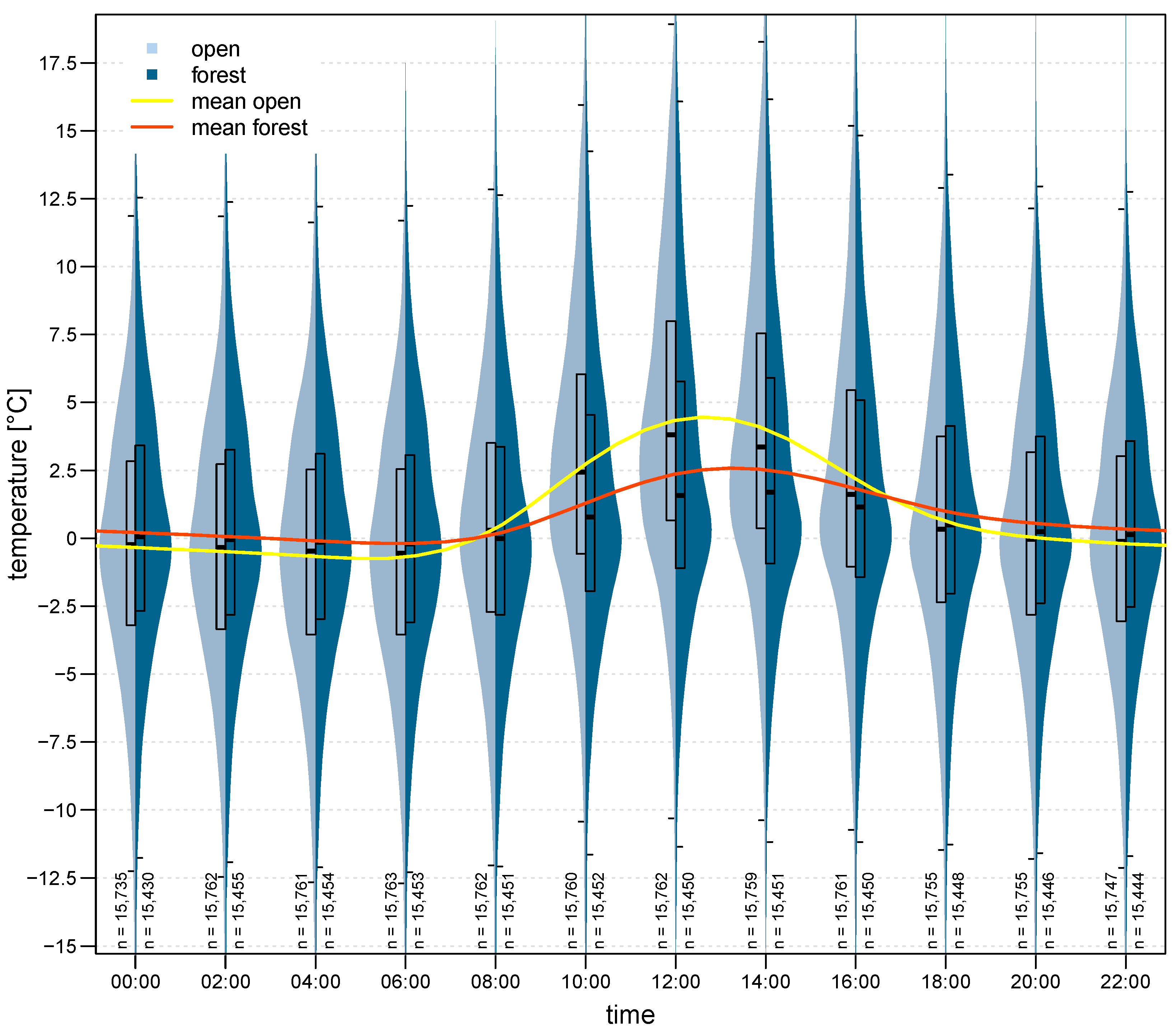
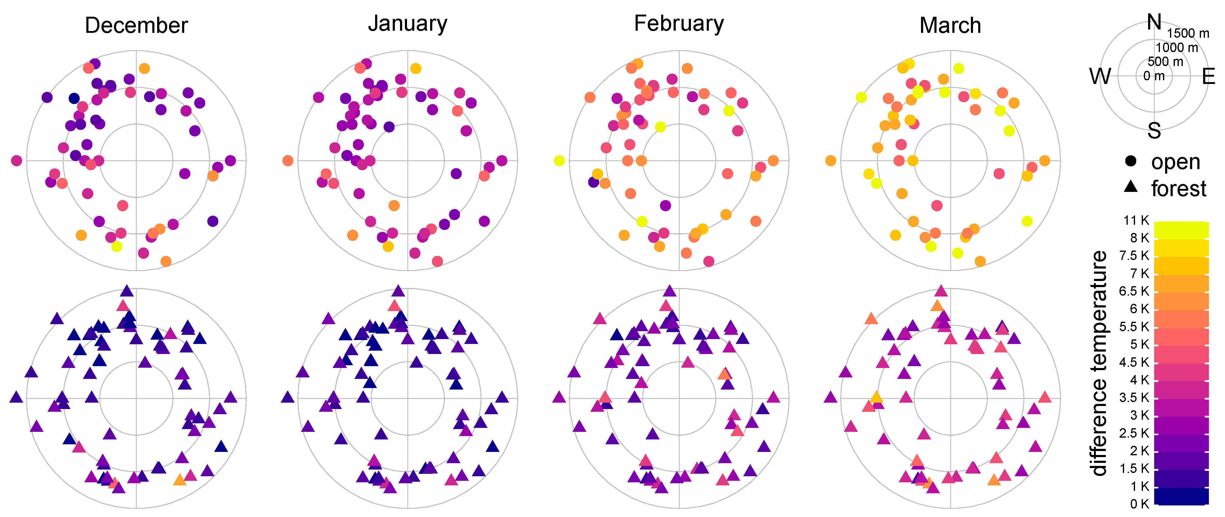
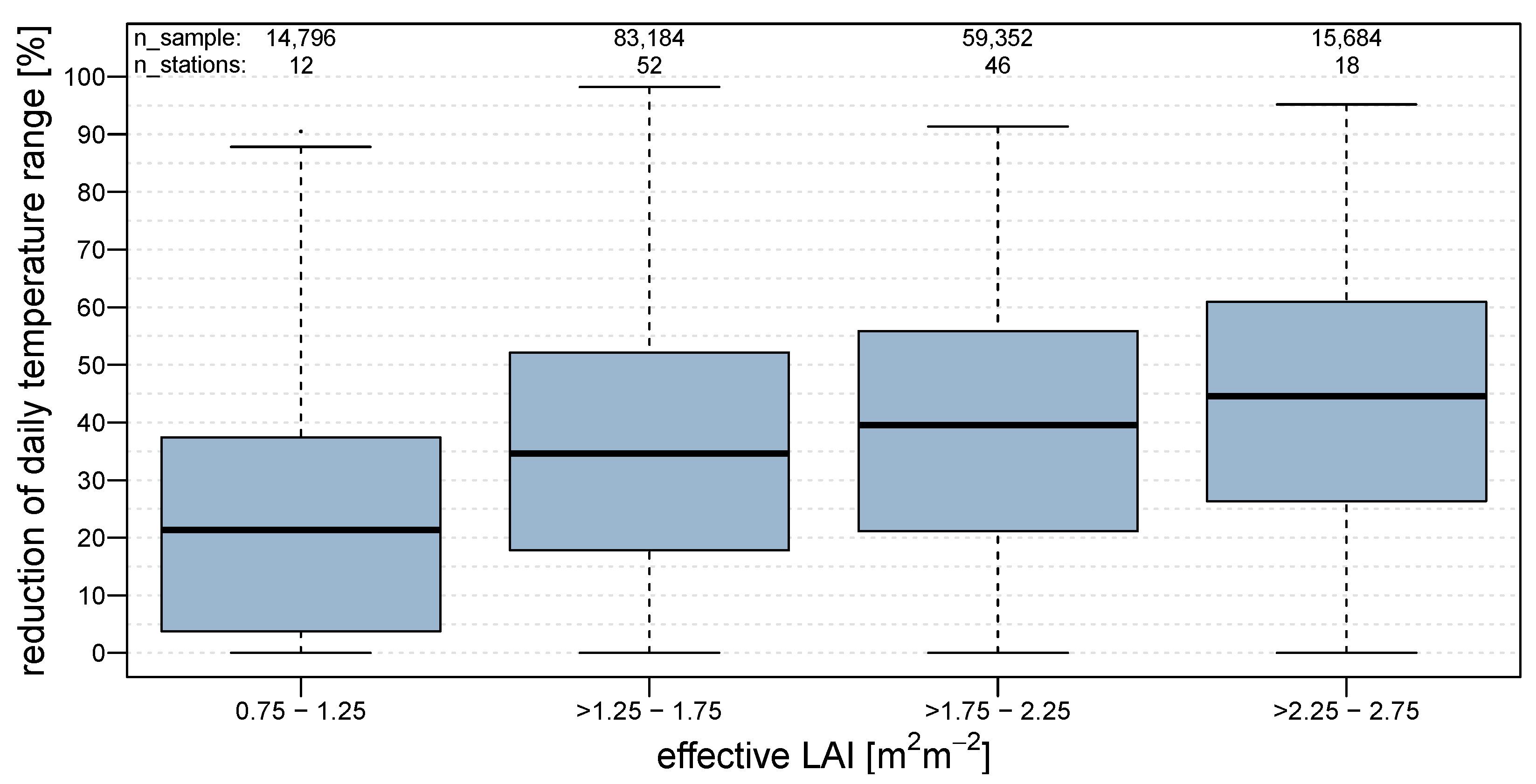
The presented dataset enables a detailed investigation of relevant processes affecting the differences measured at forested and open locations. The diurnal air temperature profile (see Figure 3) clearly confirms the common knowledge for temporal dampening in the forest. The temperature reduction due to the effective LAI (see Figure 4) also shows a clear trend. The first and the last LAI classes (effective LAI less than 1.25 m²m⁻² and effective LAI more than 2.25 m²m⁻²) contain 12 respectively 18 out of 128 station pairs, which occurs because the class boundaries have been set with an equal size for all classes and most LAI values are in between. Nevertheless, the sample size of 14 796 for the smallest class is still relatively high. When comparing the differences between the air temperatures at 04:00 and 12:00 o’clock, throughout the season (see Figure 5), it has to be mentioned that in March, data are partly limited due to instrument failure (limited energy support). The trend for higher daily air temperature ranges at the southern exposure, which occurs due to higher short-wave radiation, can be clearly seen. Furthermore, it is evident that in February and March the exposure of open stations seems to be less important compared to December and January. The reason for this could be the higher position of the sun during the day. The elevation does not seem to have an influence on the temperature difference, which makes sense, because no absolute air temperature values are shown in the plot.

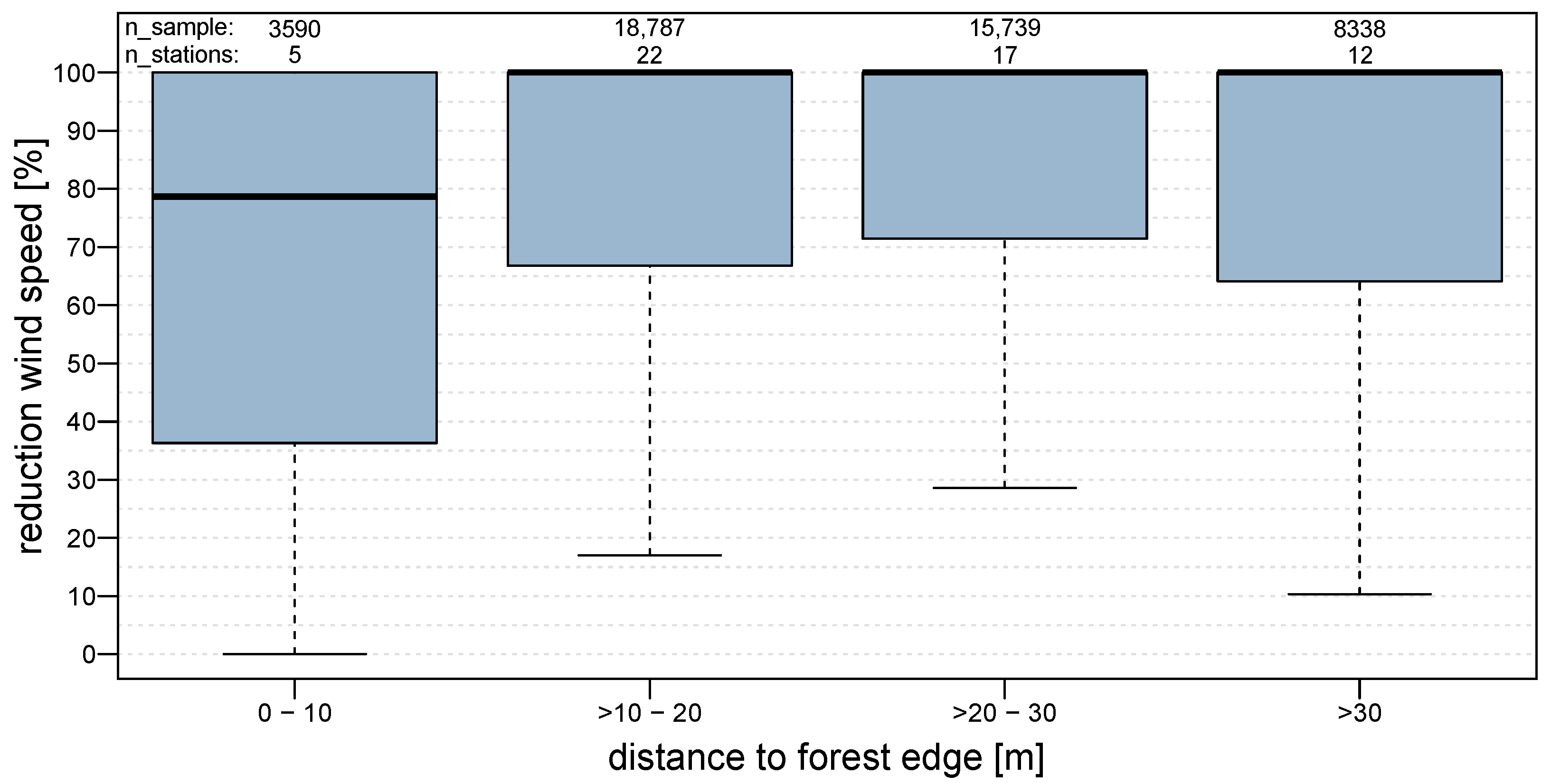
Looking at the relation between wind speed reduction and the distance of the forest station to the forest edge (see Figure 6), the first three distance classes reflect a clearly increasing reduction of wind speed due to higher distances to the forest edge. The last class, with distances above 30 m, does not confirm a further decrease in wind speed. Several reasons could be held responsible for this observation: The stations have a wide range of distances with 35–80 m to the forest edge, where it can be questioned whether it is useful to organize them in the same class. However, increasing the number of classes would lead to classes containing only one single station and consequently to a loss of statistical significance. Another point is that eight out of these 12 stations have elevations greater than or equal to 1200 m a.s.l., which is fairly high compared to the remaining station pairs. At higher elevations, forest density tends to be generally lower. Therefore, the exposure to wind speed is potentially higher, suggesting that the reduction of wind speed is lower at those locations.

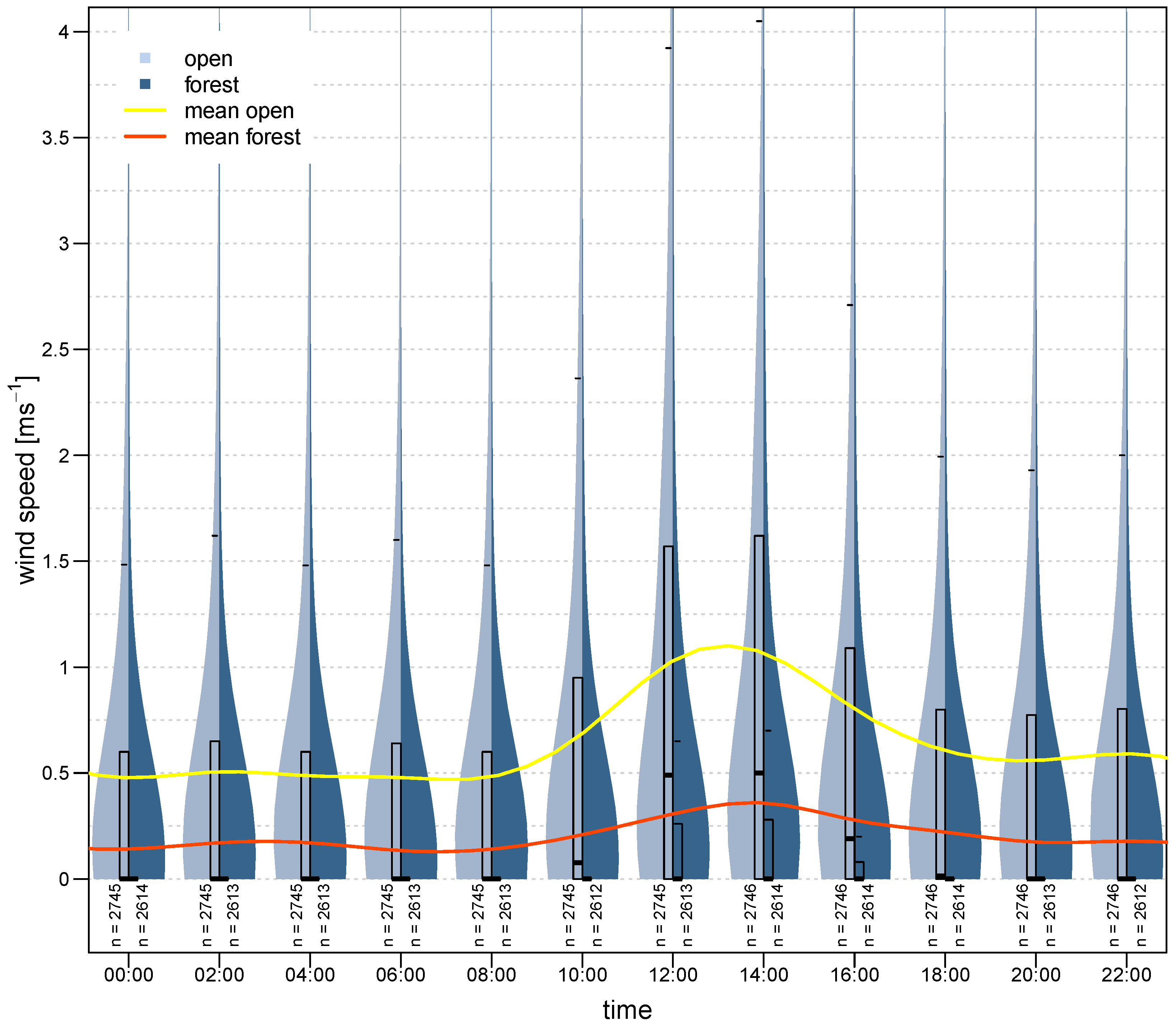
The diurnal course of wind speed (see Figure 7) allows some assumptions about the importance of short-wave radiation with regard to wind speed. The violins and boxes clearly suggest an offset for open stations between 10:00 and 16:00 o’clock, so the deviation could be related to radiation (wind effects due to surface warming etc.). The remaining wind speeds in the open stations, with a mean of around 0.5 ms⁻¹, and in the forest stations, with a mean of about 0.2 ms⁻¹, determine the average wind speeds that occur without radiation. The upper limit of the box of the forest stations is often 0, which confirms that calm situations in the forest are prevalent, or the measuring instruments have a certain minimum resistance until they record values.

When looking at the existing transfer functions, it is noticeable that, compared to the complexity of the interactions of a forest canopy with the atmosphere, very simple approaches are chosen for the description of the meteorological variables in the forest. The transfer functions are mostly only dependent on the effective LAI, which is often converted to a factor $F_c$, because this includes a logarithmic reduction. It is a great advantage that the transfer functions are kept relatively simple and depend on few parameters. The applicability to a large number of datasets is, thus, greater. However, the transfer functions are developed on the basis of a few datasets, which is why their validity might depend on the climatic conditions of the site for which fitting the functions has been conducted.

The methodological core of the development of new transfer functions lies in cross-validation. Here, the extensive dataset offers further advantages, because validation is possible at individual stations and yet a huge set of values (128 stations with 173,682 measurements for air temperature and 64 stations with 115,211 measurements for wind speed) are included for the development of the functions. The omitted samples differ in the number of meteorological values, which must be considered when evaluating the functions against the efficiency criteria. The mathematical comparability between the pairs of stations is, therefore, not given in a strict sense, but the advantage remains that completely independent stations can be used for the validation of models and, thus, its validity is strengthened.

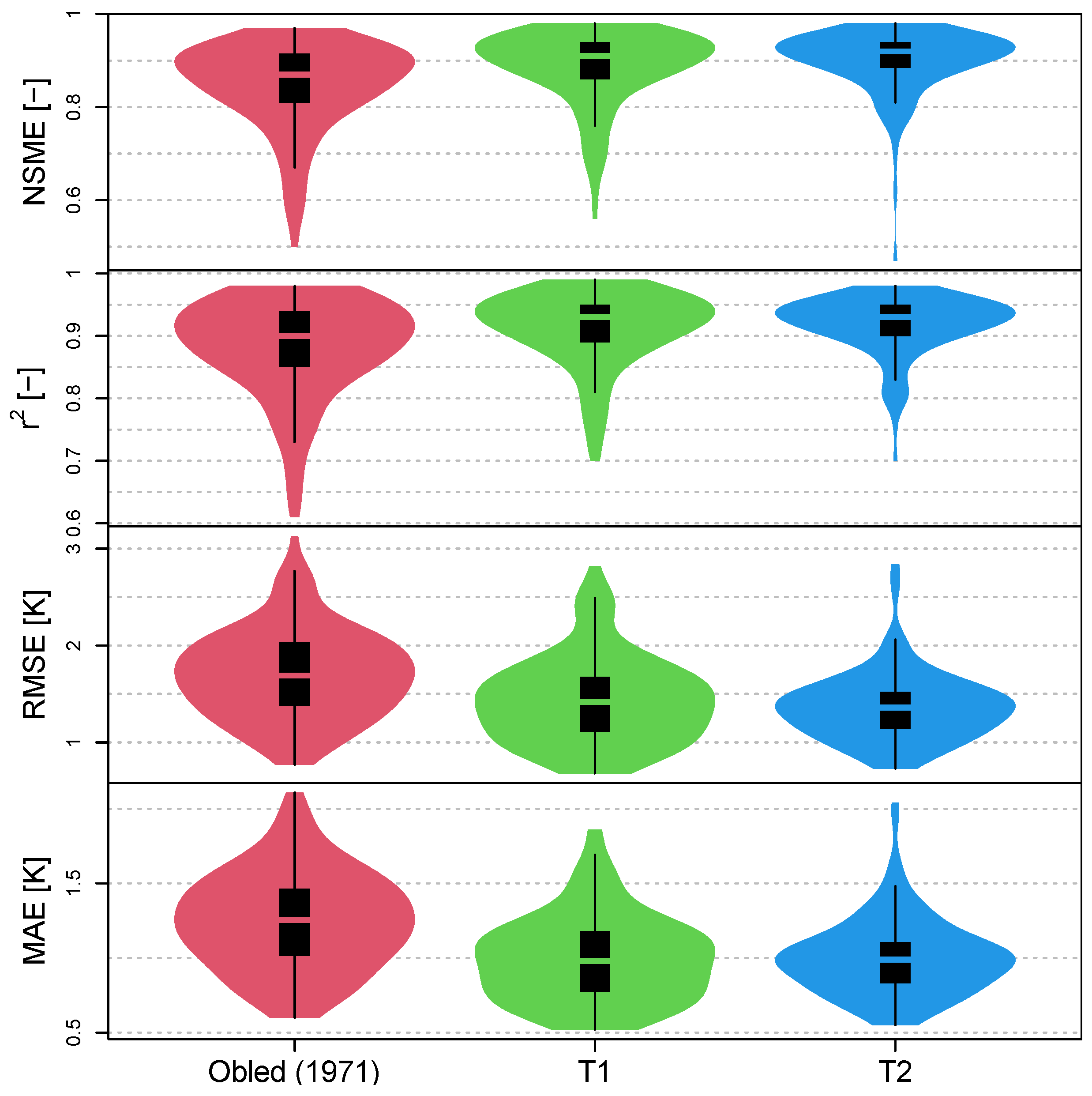
When applying the transfer functions from the literature, the strengths and weaknesses of these become apparent. The incompleteness of the data is one reason for outliers in the efficiency criteria. In addition, when evaluating the RMSE and the MAE, the range of the respective meteorological variable must be taken into account. In case of air temperature, it can be seen that the measured values are accurate and of high quality because the efficiency criteria achieve good values (see Figure 8 and Table 4). One reason could be that the air temperature is not subject to such large fluctuations over the distance between the measuring stations as, for example, wind speed. The dampening of the daily fluctuations was found to be the most challenging part because of different dampening effects during day and night. The problem of the existing transfer function is that the daily maximum and minimum values are poorly represented. To overcome this deficiency, a parabolic function is tested. With air temperature values at the upper or lower edge of the daily range, the temperature in the forest is dampened depending on the difference between the air temperature and the daily mean value in the open field. This dampening approach is a more effective way of representing the daily minimum and maximum air temperatures in the forest. Moreover, it makes sense to use the daily mean value in the field as starting value for constructing the corresponding diurnal course in the forest to keep the structure of the equation simple, because the mean values in the forest and outside are very close to each other with 0.84 °C and 0.99 °C. Additionally, daily mean values in the forest can be estimated via a previous linear regression for a more accurate starting value, but it means more computation steps and slightly higher complexity. Particularly in very cold months, the mean air temperature in the forest is even greater compared to the open field, why further refinements of details could result in better simulations in deep winter.

A further linear regression creates a strong dependence to the dataset, wherefore the scaling factor $A$ can be seen as critical already. It has to be mentioned that regarding different datasets, it is possible that equation T1 yields better results. Nevertheless, the function offers an improvement when compared of the original approach.

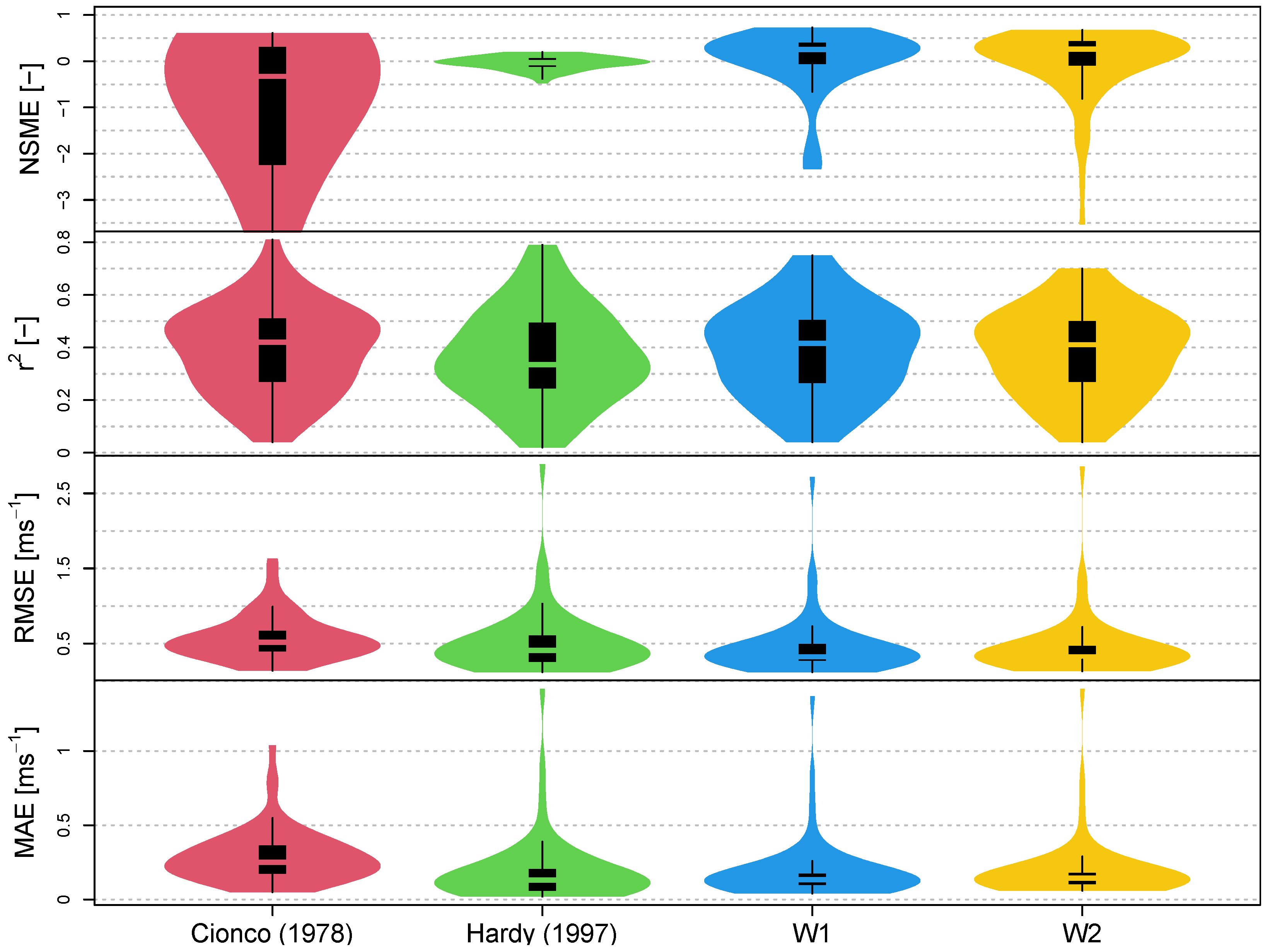
For wind speed, it is noticeable that for the existing transfer functions, the simplest approach works best (see Figure 9 and Table 5). A reason for this might be that wind speeds observed in the open field are determined by the logarithmic wind profile above a surface, which differs to the wind profile above the forest, due to differences in roughness induced coupling to the atmosphere. Thus, we are dealing with two different wind speed profiles when transferring wind speed from the open field to the forest and complex algorithms exceed their comparability. For this reason, it proves to be more reliable that only a proportion of the wind speed in the open field is assumed for the forest. The results of the efficiency criteria for the new transfer functions show NSME values around zero, suggesting that the mean value of the observations works just as well as the presented new transfer functions. From our selection of transfer functions, it is noticeable that it is hardly possible to say clearly which function performs best, which is why the approach according to Hardy et al. [25] with an exponent is chosen because it, thereby, works significantly better at high wind speeds.

When developing new transfer functions, one goal is that they are applicable and transferable to as many datasets as possible. Both the dataset and the methodology are crucial to derive new functions. The dataset introduced in our study has advantages and disadvantages. On the one hand, it is very extensive and reflects a wide range of study areas. On the other hand, its subject to measurement uncertainties. Due to the low-cost station approach used in the measurement campaigns, a lower accuracy is accepted here, since the focus of this study is put on spatial variability rather than on collecting high accuracy data for selected single sites. This way, the amount of data collected can be increased in principle at low costs to even increase the variability in the dataset. Compared to related datasets, which formed the basis for the named existing transfer functions, the dataset reflects a high spatial and temporal variability, because six different study sites are considered and data from up to six years are available.

In relation to the meteorological data, on average about 10% of the values are missing due to temporal instrument or measurement failure. The recording periods of the different stations also differ. These factors can lead to more values being available for some periods in a winter season than for others, suggesting that a higher weight is given to some seasons in the process of deriving the functions. In addition, the meteorological data in the field are not collected above the canopy, but at nearby open areas, resulting in a certain horizontal distance for each pair of stations. In some cases, measuring stations from the open field are assigned to several stations in the forest in order to increase the number of available station pairs for analysis. This can help to take the diversity of different locations into account, but it can also lead to less significance while developing new transfer functions. In general, the characteristics of the dataset are still viewed helpful, because the extensive range of values means that functions in general and fitting the functions to the dataset relies on station pairs in different environments.

5. Conclusions

The influence of a forest canopy on near-ground air layer micrometeorology is based on interactions between the trees and the atmosphere as well as shading effects. The air temperature profile in the canopy is dampened, which means that temperature amplitudes occurring in the open field are less pronounced in the forest. High air temperatures are attenuated because there is less radiation in the forest. Low air temperature amplitudes are attenuated by the long-wave radiation emission by the trees and reduced aerodynamic coupling. Wind speed is significantly reduced in the canopy. The canopy density and the tree density of the forest are important characteristics here.

Factors such as exposure and density of the forest in relation to air temperature and distance to the forest edge in relation to wind speed are considered, also supported by statistical measures such as correlation. During deep winter (December and January), the dampening of air temperature is more visible in southern exposures, while the dependence of the exposure on this effect decreases during February. In spring (March), the dampening can be observed most strongly, and it occurs noticeably at all exposures. Furthermore, the daily air temperature range in the forest decreases with increasing effective LAI. A dependence of the wind reduction on the distance to the forest edge is found, although stations located at the higher altitudes in the study areas with large distances to the forest do not confirm this observation. Finally, increased wind speed is observed on days with air temperature differences above 10 K most likely due to heating effects at the surface, which even translates to the forest with smaller amplitude.

Existing transfer functions for the calculation of micrometeorological data in forests are based on the same approaches, which is why the presented extensive dataset is not only helpful to study micrometeorological processes, it also represents unique data for the development of new model approaches or hypothesis testing. In the development of new transfer functions, linear and non-linear regression analyses are applied based on the method of least squares. The validation of the models is performed with a leave-one-out cross-validation. A disadvantage is a demanding computational effort, because the validation procedure has to be carried out 128 times for 128 pairs of stations for air temperature. Furthermore, the dataset cannot be stratified into comparable sections as in a standard cross-validation with training sets of equal sizes. However, this could even be viewed as an advantage, since a cross-study area validation is performed in this way, supporting the idea of transferability.

The air temperature is determined via a quadratic function, which makes the diurnal features in the forest more dependent on the values in the open field. In this way, the already good efficiency criteria are further improved. The wind speed is calculated with a further development of the function according to Hardy et al. [25]. An exponent and the factor $F_c$ are used for the reduction in the forest.

Transfer functions are very useful, since data in the forest are often not available due to a lack of observations stations. Especially snow modelling of subalpine (forested) areas requires meteorological variables in the forest, since the energy balance and, thus, the snow melt significantly differs under forest canopies compared to open sites. The water balance in the forest is also altered by interception, sublimation, drifting, and differences in snow cover. This, together with changing climatic conditions, directly affects the accumulation and melting process and, thus, the height and duration of the snow cover in the forest. The spatial and temporal variability of the presented data offers multiple possibilities for future research. Furthermore, validation of models is possible due to the spatial representativeness. The added benefit of the new transfer functions could be confirmed by their application to model snow interception (e.g., [10]).