Abstract
An initial condition that closely represents the true atmospheric state can minimize errors that propagate into the future, and could theoretically lead to improvements in the forecast. This study aims to evaluate and understand the impacts of 3DVAR on the state-of-the-art Weather Research and Forecasting (WRF) model with a two nested domains setup. The domain configuration of the model covers China with an emphasis on Guangdong province, with a resolution of 27 km, 9 km, and 3 km. Improvements in the forecasts for the Winter and Summer season of all the domains are systematically compared and are quantified in terms of 2 m temperature, 10 m wind speed, sea level pressure, and 2 m relative humidity. The results show that 3DVAR provides significant improvements in the winter case and surprisingly improvements were also found after the 48 h of the forecast. Evaluations of performance of 3DVAR in different domains and between two different seasons were done to further understand the reasons behind the discrepancies.
1. Introduction
Applying new methods to improve the accuracy of regional non-hydrostatic numerical weather prediction (NWP) has always been one of the most heavily investigated topics in the meteorological research society. To improve the model’s accuracy could be understood as reducing the errors of the model. The origin of the errors of a regional mesoscale model can be dissected into three main categories. First, errors can come from the imperfect integration method applied in maintaining the stability of the discretized model [1]. Secondly, errors can arise from the underlying physics within the model, as the parameterizations are heavily dependent on the scale of the weather phenomena that it aims to predict. Last but not least, errors can also originate from the data inputs used for generating the forecasts. With erroneous input data, even a perfect model will be prone to generating erroneous simulation results. The first two categories are more related to the internal errors that exist in the model itself; however, the last one is more related to the quality of the input data. Thus producing input data that closely resemble the true state of the atmosphere for the model is very important to generate an accurate forecast, and as essential as improving the underlying dynamics, physical schemes and the structure of model.
In order to reduce the error of the input data used for initializing the model, one of the most popular methods is to assimilate observations onto the initial atmospheric field, and this method is known as data assimilation. Kalnay [2] provides readers with a fundamental understanding of data assimilation, as well as introducing different state-of-the-art data assimilation methods that were applied and are being applied in most of the meteorological agencies. As we are aiming for an efficient and less resource-demanding data assimilation strategy, the three-dimensional variational (3DVAR) data assimilation method is considered to be the best option to be apply to the forecasting model to improve the initial condition. Numerous studies applied 3DVAR on a non-nested regional mesoscale model or a single domain ([3,4,5,6], etc.). While these studies show that 3DVAR leads to significant improvements in the initial conditions and has proven to have positive effects on the initial 48 h of forecasts, limited efforts were made to investigate the effect of applying 3DVAR to several nests of a regional mesoscale model and how it impacts the post-48 h time period of the forecasts. Additionally, most 3DVAR applications are event-based and short-term forecasting. Fan [7] applied 3 h cycling 3DVAR to a nested 27 km/9 km/3 km domain, focusing on the prediction of 0–6 h accumulated rainfall of a specific heavy rain event that occurred in Beijing, China. Jianfeng [8] targeted a specific typhoon case to evaluate the effectiveness of 3DVAR. They improved the initial condition by optimizing the background error statistics (BES) and tuning the scale-length parameter. Many other 3DVAR-related studies also aimed to investigate specific weather phenomena ([5,9,10,11], etc.). While these studies make a notable contribution to the short-term forecasting of severe weather events, they are not representative enough to demonstrate the performance of 3DVAR for general day-to-day weather forecasting.
In the Environment and Sustainability department of Hong Kong University of Science and Technology (HKUST), one of our goals is to be able to accurately predict the dispersion of pollutants within the Pearl River Delta (PRD) region, in which the atmospheric input heavily relies on the accuracy of the weather forecasting model. In order to create a more accurate atmospheric condition to drive the air pollution model, numerous methods have been researched, tested, and applied to our weather forecasting model, such as considering the frictional force induced by urban effects in the ACM2 PBL scheme [12] as well as utilizing the multi-layer urban canopy model (WRF-BEP) model [13], which provides direct information exchange between the planetary boundary layer (PBL) and the buildings. With more sophisticated building height parameters, more accurate weather forecasts could be achieved [14] within an urban landscape. However, these are improvements which reduce errors that are within the aspect of the model itself. While efforts were also spent on reducing the errors that lie within the input data, through updating the soil map and the soil moisture to improve the realism of the model regarding the latent heat energy that is stored in the ground [15], the changes regarding the atmospheric field are affected in a passive way.
With the PRD region situated within the sub-tropical region and along the coastline of South-Eastern China, the weather patterns are season-dependent. In the summer, the South-Westerly monsoon dominate. The maritime air stream brings in moist and warm air mass from the ocean towards the region. In the winter, the north-easterly monsoon, together with the southward movement of Siberian continental air-mass, brings dry and cold weather to the region. Due to the drastic difference in weather patterns, focusing on a specific weather phenomena within a particular season does not show a complete analysis of the performance of 3DVAR. Therefore, in this study, we would like to evaluate and understand how 3DVAR behaves in general, without focusing on any specific weather event, and to focus on the post-48-h impacts of applying a 3DVAR data assimilation method using conventional observations on the Weather Research and Forecasting (WRF) model, which has a two-nested domains setup.
The intention of applying variational data assimilation to any NWP model is to generate the most precise and accurate estimate, close to the true state of the atmosphere at a specific analysis time, using the iterative method to find the solution of a prescribed cost-function, such as Equation (1) [16]. In this paper, the term WRF-Var will refer to the data assimilation component, which is responsible for the minimization and iterative process that consists of Equation (1), while the term WRFDA refers to the entire WRF data assimilation system, including various other components.
The essence of the variational method is to find an analysis state that could minimize . This could be done by minimizing Equation (1) iteratively until a suitable is found, which contributes to obtaining a minimum of . With the given priori data and error matrices, such as the background state (including model error B) and the observations (including observation errors E and F), could be shown as the posteriori maximum likelihood estimate of the real atmospheric condition [17,18]. The entire data assimilation system consists of several components: observation preprocessing (OBSPROC) unit, the background error unit (gen_be utility), the WRF-Var unit, and the update lateral boundary conditions unit (WRF_BC). These processing units are supplied with various observation data and model analysis, which are then processed to generate data files to input into the WRF-Var to perform the assimilation process.
When data assimilation is applied on a regional domain, WRF-Var extends the observation information and relays it beyond its original location using recursive filters as a diffusion operator [19]. Updating the existing wrfbdy lateral boundary condition files () is an essential step and could be done via the WRF-BC utility [1]. This update process allows to remain consistent with to avoid unexpected gravity waves being generated.
The objective of this paper is to understand the sensitivity of the NWP model towards the application of 3DVAR. The paper focuses on two parts. First, the effectiveness of the application of 3DVAR on different domain setups and evaluate its contribution towards different prediction times. Second, the seasonal effects on the response of the model towards the 3DVAR application. We organized the paper in the following fashion. Section 2 (Model and data assimilation setup) would focus on the setup of the NWP model and the data assimilation protocol. Section 3 (Data) would show the data we used for both the model and the data assimilation process. Then, in Section 4 (Methodologies and Results), the methodologies of the studies would be laid out and the results of those studies would be presented. Lastly, Section 5 (Conclusions) summarizes the study by highlighting the findings of the experiments carried out in this paper.
2. Model and Data Assimilation Setup
One of the most important inputs for variational data assimilation systems is the background error covariance B. It performs several important roles in data assimilation, such as: (i) determining the weight of the background state , so that the analysis can be defined to either match the observations more or less closely; (ii) projection of the spatial and multivariate characteristics of the model error; (iii) maintaing the physical balance between variables when applying increments.
The background error can be understood as the deviation of the model from the true state of the atmosphere. However, we do not possess the information of the truth, thus refraining us from producing the true background error. Therefore, a best estimate of the true atmospheric condition () has to be produced to substitute , such that we can determine the background error via the forecast difference National Meteorological Center (NMC) method. In 3DVAR systems, the background error covariances are estimated offline and have similar characteristics to climatological statistics, which do not evolve with time, it is also not flow-dependent. This allows for a more computationally efficient NMC method to be applied. The NMC method uses forecast differences (e.g., T + 48 minus T + 24 for global model and T + 24 minus T + 12 for regional model) statistics to generate the background error covariances, with the assumption that both forecasts have the same model BIAS and uncorrelated errors [20].
The WRF model with the Advanced Research WRF (ARW) dynamical core is used for generating the simulations. A parent domain and two nested domains are applied in this research, namely, domain 1 (D1), domain 2 (D2), and domain 3 (D3). The first domain D1 focuses on converting synoptic scale weather phenomena into mesoscale- scale events that propagate through or develop within China. The second domain D2 collects information from D1 and acts as a buffer region for the conversion between mesoscale- and mesoscale- scales weather events that propagate or develop within the southeastern part of China. D3 focuses on the propagation and development of mesoscale- scale weather within the Guangdong region of China. The specifications of these three domains are listed in Table 1 and a spatial representation is shown in Figure 1. The model applied in this study was being run in parallel and the domains are one-way nested with the static terrestrial data downloaded from the WRF download website [21]. The geographical data include various geographical information which consists of the characteristics of the terrain on which the model is running. The model does not use restart and we consider the first 24 h as the spinning-up time for the model. We selected the two time periods for the model simulation, June 2015 and December 2015. In general, they represent the summer season and the winter season for our study, respectively, and in some experiments, only the winter season was evaluated (Section 4).

Table 1.
The general configuration of the parent and the child domains of the WRF model.
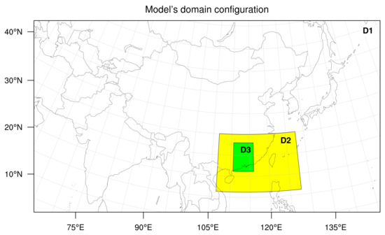
Figure 1.
The domain configuration of the model. There are a total of 3 domains with 2 nests. Domain 1 (27 km) is being shown as D1, domain 2 (9 km) is being shown as D2, and domain 3 (3 km) is being shown as D3.
The WRF Data Assimilation (WRFDA) System is being used for the data assimilation process and the gen_be utility is used to generate the background error covariances (BE) via the NMC method. One month of 12 h initiated WRF simulation data, set prior to the study period, are supplied to the gen_be_wrapper to estimate the forecast error covariance CV5 [27]. Two sets of BE are generated, one for the summer and the other for the winter. Together with the BE, the observations are assimilated onto the initialization timestep with a window size of 10 min to maximize the usable data. We increased the VAR_SCALING (VS) of all the variables from 1.00 (default) to 3.00, following [28]. The increase in VS is mainly because the error of the model error is generally underestimated, as shown in [11,29,30]. Since observations that lie above five of the error covariance are automatically rejected, the increase in VS increases the underestimated model error, thus allowing more observations to be assimilated into the model.
- VAR_SCALING1 = 3.00, 3.00 (ψ)
- VAR_SCALING2 = 3.00, 3.00 (χu)
- VAR_SCALING3 = 3.00, 3.00 (T_u)
- VAR_SCALING4 = 3.00, 3.00 (rh)
- VAR_SCALING5 = 3.00, 3.00 (Psfc_u)
3. Data
The data used for the WPS unit of the WRF-ARW and WRFDA data assimilation system are described as follows.
Meteorological data: WPS requires an external meteorological source to provide atmospheric information to initialize the simulation. In this research, we use the NCEP operational Global Forecast System (GFS) analysis and forecasts, as the initial meteorological fields for the simulation. The data are 0.25 degree resolution, which has time steps at a 3-h intervals from 0 h to 240 h, initiated at 00, 06, 12, and 18 UTC daily, stored as GRIB2 format. The GFS analyses contain various variables, which include air temperature, albedo, cloud frequency, cloud liquid water/ice, sea surface temperature, skin temperature, soil temperature, upper air temperature, vorticity, etc. More information about the dataset can be found in [31].
Two sets of observation data are applied in this research and they serve a different purpose during the simulation process. The two sets of observation data will be described as follows:
(1) NCEP ADP Global Upper Air and Surface Weather Observations (ds337.0): These datasets are provided by the National Centers for Environmental Prediction (NCEP), and they compose of a set of global operational surface and upper air reports. The observation data are reported at a time interval ranging from 1 to 12 h. All the data are stored in the PREPBUFR format, while ASCII and NetCDF formats are also available [32]. Each observation in the dataset comes with a quality marker (qm), and a qm less than 3 are kept to ensure that good-quality observations are assimilated in this study. All the observations which passed the QC and are within the domain of our study are assimilated into the initial condition;
(2) The Environmental Central Facility Atmospheric and Environmental Database: These datasets are provided solely for educational and research purposes, by the Environmental Central Facility (ENVF) within the Institute for the Environment (IENV) of the Hong Kong University of Science and Technology (HKUST). They comprise reports of conventional surface observations gathered from GTS, Meteorological Terminal Aviation Routine Weather Report (METAR), and Surface Synoptic Observations (SYNOP), and the data went through several quality control measures. More information regarding these datasets can refer to [33]. The purpose of these observation data is to evaluate the result of simulations both before and after 3DVAR which are applied to the model, so that we can understand the changes made by the data assimilation system, with the assumption that the observations used by WRF-VAR for the data assimilation and the observations used to evaluate the results are uncorrelated with each other. We selected four variables—2-m surface temperature, 10-m zonal and meridional wind, and 2-m relative humidity—as the variables for the evaluation process. In this research, since we are mostly interested in the behaviour of the model within the Pearl River Delta region, some of the evaluation on the middle domain (domain 2) would be shown for a more complete study, but only the outermost domain (domain 1) and the innermost domain (domain 3) would be evaluated in detail. All results were evaluated by the observation data located within the Guangdong province (Figure 2), except the evaluation on the 27 km domain for the seasonal sensitivity study (Figure 3).
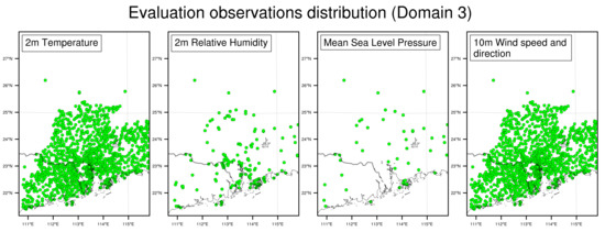
Figure 2.
The distribution of the observation data that are used to evaluate the performance of the model. All the observations are situated within the Guangdong province which is covered by domain 3 (D3) of the model (Figure 1).
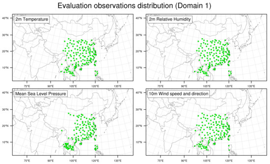
Figure 3.
The distribution of the observation data that are used to evaluate the performance of the model of domain 1 (D1) for seasonal sensitivity forecast (Figure 1).
4. Methodologies and Results
4.1. Background
The results are analyzed in terms of how sensitive the model is with the application of 3DVAR and they can be separated into three parts, namely, domain sensitivity, which is the sensitivity of the domain’s reaction towards the application of 3DVAR, time period sensitivity, which is the sensitivity of the model at different time period of the simulation, and seasonal sensitivity, which is the sensitivity of the model, with 3DVAR application, towards the change in atmospheric conditions due to seasonal variations. Thus, two studies, namely the general (domain and time period) sensitivity study and seasonal sensitivity study, meaning that information from the child would not pass back to the parent; thus, observations assimilated in the child domain should also be assimilated again on the parent domain. Nearest grid point prediction value is used to calculate the evaluation metrics.
4.2. General Sensitivity Study
This general sensitivity study aims to understand the effectiveness of 3DVAR on different domains and time periods of a model run. Four cases were conducted in this experiment, as shown in Table 2. A Control case (CONTROL_DOMAIN) was run without applying 3DVAR to any of the domains so that the performance of the model without 3DVAR application can be used as a reference for comparison. The second (3DVAR_DOMAIN_D1), third (3DVAR_DOMAIN_D12) and forth (3DVAR_DOMAIN_ D123) cases apply 3DVAR on Domain 1 only, Domains 1 and 2, and Domains 1, 2 and 3, respectively. The data assimilation and simulation settings used the same settings as mentioned in Section 2. The BE was generated using a month-long simulation of November 2015 via the NMC method of WRFDA. Four days of hourly WRF forecasts are initiated, using the NCEP GFS analysis by WRF Standard Initialization (WRF_SI) as the control case (CONTROL) or WRF_SI plus WRFDA (3DVAR_DOMAIN cases), every 24 h, from 1200Z of 1 December 2015 to 31 December 2015. The results of domain 1 and domain 3 of the cases are compared against the reference case (CONTROL) and the effectiveness of the application of 3DVAR on the designated domains are examined based on the scale of improvements in the initial condition, as well as the result of the forecasts compared with the ENVF observation dataset, using BIAS and RMSE statistical evaluation methods. Four evaluation metrics were used, namely, (Equation (2)), (Equation (3)), (Equation (4)), and (Equation (5)), where the subscript “time” indicates that the metric is calculated along the forecast period for each validation station, while the subscript “station” indicates that the metric is calculated across all the validation stations for each forecast hour.
where:

Table 2.
The application of 3DVAR for the general sensitivity study. ✗ refers to 3DVAR not being applied and ✓ refers to 3DVAR being applied.
- Pi = Prediction value
- Oi = Observation value
- n = Number of forecast hours
- s = Number of stations
4.2.1. Domain Sensitivity Experiment
A total of four cases, three with 3DVAR and one without, as shown in Table 2, were evaluated on all three domains. The observations we used for the comparisons are 2 m temperature (T2), 2 m relative humidity (RH2), sea level pressure (SLP), and 10 m wind speed (10 m wind).
Figure 4a,b shows the distribution of and of all stations. It is clear that the 3DVAR_DOMAIN_D1 enjoys the greatest benefit from the application of 3DVAR. The differences between CONTROL_DOMAIN and 3DVAR_DOMAIN_D1 is the greatest among all other 3DVAR cases. The mean is always being shifted more closely towards 0 and the mean is mostly being reduced. Among all the variables, 2 m temperature sees the most significant improvements, as the mean sees a correction of +0.68 C and +0.51 C for 27 km and 3 km domain, respectively. The is also reduced by 0.31 C in the 27 km domain, with the entire distribution shifting lower. Further applying 3DVAR to domain 2 (3DVAR_DOMAIN_D12), the improvements are less significant compared to those seen with the application domain 1 only (3DVAR_DOMAIN_D1). Even though the improvements are small, the mean are generally shifted closer to 0, with lower mean values. If we continue to apply 3DVAR towards domain 3, we could see negligible improvements. The results show that there is an inverse relationship between the application of 3DVAR and nested child domains. The more you apply 3DVAR on child domains, the fewer improvements there will be. This experiment shows that, with the given setup, the most effective data assimilation configuration would be the application of 3DVAR on domain 1 and 2 only (3DVAR_DOMAIN_D12). Having shown that 3DVAR_DOMAIN_D12 is the most effective configuration, in the following sections, instead of showing the statistics of all the cases, we would be focusing on comparing between CONTROL_DOMAIN and 3DVAR_DOMAIN_D12, and show their respective differences.
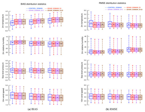
Figure 4.
The distribution statistics of the and for variables 2 m temperature, 2 m relative humidity, sea level pressure, and 10 m wind speed for all the general sensitivity study cases [CONTROL_DOMAIN (leftmost), 3DVAR_DOMAIN_D1 (center-left), 3DVAR_DOMAIN_D12 (center-right), 3DVAR_DOMAIN_D123 (rightmost)] evaluated at the 27 km (left), 9 km (center) and 3 km (right) resolution domains.
4.2.2. Time Period Sensitivity Experiment
In this experiment, we look at the and which are the metrics that averaged of the validation stations along the forecast period. Taking a closer look at of 2 m temperature and 2 m relative humidity of the 27 km domain in the Figure 5a, we observe that there are dramatic improvements in at the beginning of the model due the application of 3DVAR but diminished quickly within the first 24 h of the model run. The diminishing property is within expectations with Barker [18], and Hou [5] also show similar diminishing results in their forecast runs. The main reason which causes the retrograding effect within the first 24 h is that when the model approaches towards the 24 h mark, the boundary effect takes over the effects brought by the initial condition, which ultimately becomes the major factor in driving the model’s forecast. Since only the initial condition and the initial boundary condition is improved, the model will have a tendency to follow a track similar to a pre-3DVAR forecast, due to the predetermined information contained within the unimproved boundary layer of the parent domain.
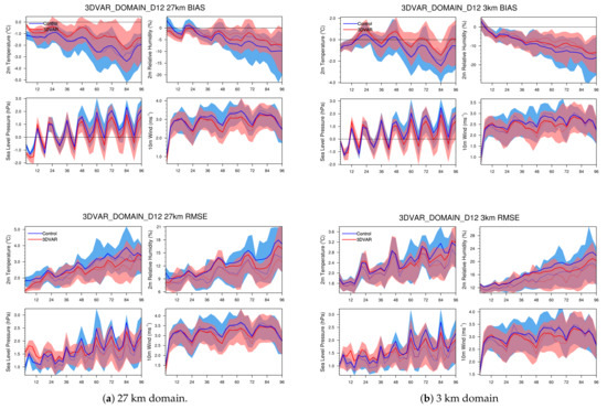
Figure 5.
The and statistics of 3DVAR_DOMAIN_D12 (red) comparing to the control case CONTROL_DOMAIN (blue) for the 27 km and 3 km domain. The solid lines represent the mean, the dotted lines represent the median and the shaded areas indicate the upper and lower quartile of the distribution. The statistics of the variables 2 m temperature, 2 m relative humidity, sea level pressure, and 10 m wind speed are shown.
The previous research rarely shows the effects of 3DVAR after the 48 h time period, mainly due to the lack of interest in the post-48-h time period or due to the assumption that 3DVAR mainly provides plausible improvements within the first 24–48 model hours. To our surprise, we found that the effect of 3DVAR is not totally replaced by the boundary layer information; instead, some improvements are sustained after the 48 h time period. From Figure 5a the results show that, in the 27 km domain, observable improvements in both the and can be found between 48 and 96 h of forecast. The difference in the mean and the span between 3DVAR_DOMAIN_D12 and CONTROL_DOMAIN continues to grow towards the end of the simulations, indicates that the improvements, due to the application of 3DVAR, grows instead of diminishing. Since 3DVAR is not applied on the 3 km domain, there is no initial enhancement. All the improvements appear in this domain are solely due to the enhancements made in 27 km and 9 km domain, which is then passed in. From Figure 5b), all variables show a certain degree of improvement. The of the 2 m temperature and 10 m wind are improved after 12 h of forecast, which shows that these variables are the most sensitive towards the changes made by 3DVAR. While the improvements under 2 m temperature are sustained throughout the simulation, improvements under 10 m wind were only sustained until 72 h of forecast. Regarding the , the 10 m wind reacts the quickest to changes made by 3DVAR, with the greatest improvements between 24 and 72 h of forecast. Although 2 m temperature and 2 m relative humidity also show improvements, they appear to occur mostly after 48 h of forecast. Figure 6a,b shows the and the distribution statistics for the all the cases between 48 and 96 h of forecast. From these figures, one could easily observe that there are some degrees of improvement regarding or on all of four variables, with 2 m temperature and 2 m relative humidity being the better performers. Looking at the numbers, Figure 7a shows the percentage of improvements in of 27 km and 3 km domain. Other than 10 m wind, all other variables have at least a 20% improvement, with 2 m temperature having a 40% of improvement in the 27 km domain and 65% of improvements in the 3 km domain. Figure 7b shows the percentage of improvements in of 27 km and 3 km domain. In the 27 km domain, where 3DVAR is applied, the improved, on average, by more than 10% for 2 m temperature, 6% for 2 m relative humidity and sea level pressure, and 4% for 10 m wind. Regarding the 3 km domain, the mean generally improved by 4% to 8% for all variables. The surprising results show that the improvement in 3DVAR is not constrained within the first 24 h of model runs. It has the potential to provide significant improvements after 24 h of simulation runs.
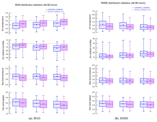
Figure 6.
The distribution statistics of and for variables T2, RH2, SLP, and 10 m wind for all the time period sensitivity experiment cases [CONTROL_DOMAIN(left), 3DVAR_DOMAIN(right)] between the 48 and 96 h time window, evaluated at the 27 km (left), 9 km (center) and 3 km (right) resolution domains. The blue dots refer to the mean.

Figure 7.
The percentage improvements of and for the case 3DVAR_DOMAIN_D12, comparing to CONTROL_DOMAIN.
4.3. Seasonal Sensitivity Study
4.3.1. Background and Setup
The seasonal sensitivity study is the extension of the first study (General sensitivity study). Seasonal variations are a major factor affecting the performance of 3DVAR data assimilation, as the dynamics of the monsoon affecting the winter and the summer season in the South Eastern China differ greatly. Therefore, it is essential to understand how 3DVAR performs in different seasons. In this study, we selected December 2015 as the simulation period for the winter case and June 2015 as the simulation period for the summer case. Four cases, namely, CONTROL_SUMMER, CONTROL_WINTER, 3DVAR_WINTER, and 3DVAR_SUMMER, are used to evaluate the seasonal performance of 3DVAR, where CONTROL_WINTER, 3DVAR_WINTER are duplicates of the cases CONTROL_DOMAIN and 3DVAR_DOMAIN_D12 used in the general sensitivity study. The data assimilation and simulation settings of the four cases use the same settings mentioned in Section 2. For the 3DVAR_SUMMER and 3DVAR_WINTER cases, 3DVAR is applied only on the 27 km and 9 km domain base (similar to the settings of 3DVAR_DOMAIN_D12) on the result of the domain sensitivity study. Four days of hourly WRF forecasts are initiated, using the NCEP GFS analysis by WRF_SI (CONTROL) or WRF_SI plus WRFDA (SUMMER/WINTER cases), every 24 h, from 1200Z of 1 June 2015 to 30 June 2015 for the summer cases, and every 24 h for 1200Z of 1 December 2015 to 31 December 2015 for the winter cases. The simulation results of the 27 km and 3 km domain of the 3DVAR_SUMMER and 3DVAR_WINTER cases are compared with the reference cases CONTROL_SUMMER and CONTROL_WINTER between the 48 and 96 forecast hours, to understand the performance of the model with and without 3DVAR application. The results of the forecasts of the 3DVAR applied cases are also be cross-compared with the ENVF observation dataset, using various statistical and spatial analyses methods. From hereonin, we would refer to CONTROL_DOMAIN as CONTROL_WINTER and 3DVAR_DOMAIN_D12 as 3DVAR_WINTER, and, since the results have been shown in the previous section (time period sensitivity experiment), they ware not be presented again in this section. In this section, we emphasize the results of the summer case and compare the improvements between the CONTROL_SUMMER and 3DVAR_SUMMER cases.
4.3.2. The Summer Case Result
Figure 8a,b shows the difference between CONTROL_SUMMER and 3DVAR_SUMMER, and we can quickly observe that the model has a consistent cold and overestimates the 2 m relative humidity, which is very similar to that in the winter case. However, the improvements are marginal compared to 3DVAR’s performance in the 3DVAR_WINTER case. ck intended meaning has been retained. In the 27 km domain, we could observe improvements in of 2 m temperature and 2 m relative humidity in the first 12 h of simulation, which corresponds to most of the literature, but converges quickly towards CONTROL_SUMMER. If we look more closely at the 48–96 h time period (Figure 9a,b and Figure 10a,b), where major improvements were found in 3DVAR_WINTER, we see that, in the 3DVAR_SUMMER cases, there are minor but insignificant improvements for 2 m temperature ( and ) and 2 m relative humidity ( only). Even though the mean of 2 m relative humidity performs quite poorly, with a more than 15% decrease in performance, the error is less than 1% in magnitude. Sea level pressure, vastly different from that in the winter, is a consistent poor performer in the summer time. In general, the application of 3DVAR does not worsen the performance of the model but nor does it provide benefits to improve the model’s performance in the summer period of the model simulation.
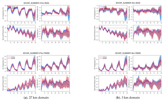
Figure 8.
The and statistics of 3DVAR_SUMMER (red) comparing to the control case CONTROL_SUMMER (blue) for the 27 km and 3 km domain. The solid lines represent the mean, the dotted lines represent the median and the shaded areas indicate the upper and lower quartile of the distribution. The statistics of the variables 2 m temperature, 2 m relative humidity, sea level pressure, and 10 m wind speed are shown.
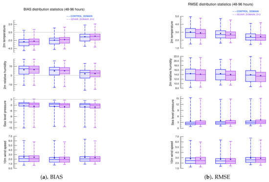
Figure 9.
The distribution statistics of and for variables T2, RH2, SLP, and 10 m wind for all the time period sensitivity experiment cases [CONTROL_DOMAIN(left), 3DVAR_DOMAIN(right)] between the 48 and 96 h time window in the summer. The blue dots refer to the mean.

Figure 10.
The percentage improvements of and for the case 3DVAR_SUMMER, comparing to CONTROL_SUMMER.
4.3.3. Seasonal Comparison
The application of 3DVAR on WRF at different seasons produces significantly different results. In both the winter and summer seasons, WRF has a cold when the forecast is 2 m temperature and the underestimation of 2 m relative humidity is more serious in winter than in summer. In the winter season, those large in the 2 m temperature were significantly improved and the is also reasonably improved. However, in the summer season, the of the 2 m temperature is not improved, nor is the . Most of the errors that exist in CONTROL_SUMMER were passed onto 3DVAR_SUMMER with unnoticeable changes. In order to understand the reason behind the huge discrepancy between these two cases, the spatial difference between the 3DVAR cases and the control cases, and the general wind pattern have to be examined.
Figure 11 shows the 2 m temperature and 2 m relative humidity monthly averaged difference between 3DVAR_WINTER and CONTROL_WINTER. The averaged spatial differences and the averaged wind speed and direction are plotted every 24 h. The purple box is where the evaluation observations for evaluating the 27 km domain are located (Figure 3) and the green box is where the evaluation observations for evaluating the 3 km domain are located (Figure 2). 3DVAR mainly increased the 2 m temperature and the 2 m relative humidity of the inland area. With the wind blowing from inland towards the sea and the wind direction at the upper latitude mainly parallel to that of the northern boundary layer, the boundary layer does not appear to provide an extensive amount of new information to the domain. Although the effects of 3DVAR become weaker between 24 and 48 h, the increments from 3DVAR still persist, as changes from the 3DVAR process are still preserved. After 48 h, the wind direction allows the effects of 3DVAR to be propagated into the 27 km domain’s evaluation zone and the 3 km domain. These results correspond to the reduction in and in the 3 km domain after the 48 h period, shown in Figure 5b.
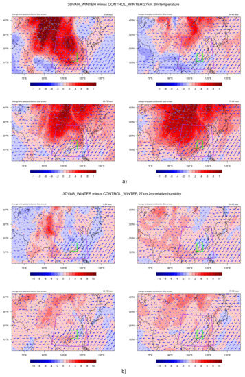
Figure 11.
The contour plots show the difference of the (a) 2 m temperature and (b) 2 m relative humidity at four different time periods, (1) 0–24 h, (2) 24–48 h, (3) 48–72 h, and (4) 72–96 h, between the 3DVAR_WINTER and the CONTROL_WINTER in the 27 km domain. The blue arrows indicate the monthly averaged wind speed and direction of CONTROL_WINTER to show the general wind pattern of this season. The purple box is where the evaluation observations for evaluating the 27 km domain are located (Figure 3) and the green box is where the evaluation observations for evaluating the 3 km domain are located (Figure 2).
Figure 12 shows the 2 m temperature and 2 m relative humidity monthly averaged difference between 3DVAR_SUMMER and CONTROL_SUMMER. It can be seen that the 3DVAR has the majority of effects in the inland. However, different from that of the winter case, the wind in the summer case blows from the sea towards inland and the wind direction along the boundary layer suggest that an extensive amount of new information is fed into the domain via the boundary condition. Due to this, the effects of 3DVAR quickly dissipate and the effects of 3DVAR after the 24–h forecast are very insignificant.
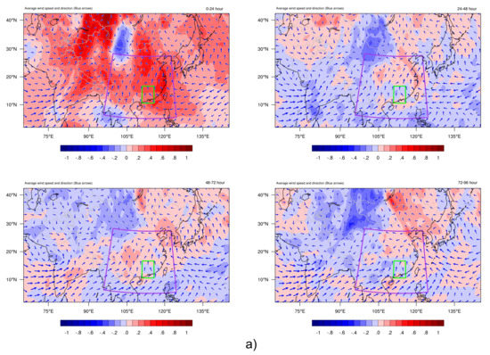

Figure 12.
The contour plots show the difference of the (a) 2 m temperature and (b) 2 m relative humidity at four different time periods, (1) 0–24 h, (2) 24–48 h, (3) 48–72 h, and (4) 72–96 h, between the 3DVAR_SUMMER and the CONTROL_SUMMER in the 27 km domain. The blue arrows indicate the monthly averaged wind speed and direction of CONTROL_SUMMER to show the general wind pattern of this season. The purple box is where the evaluation observations for evaluating the 27 km domain are located (Figure 3) and the green box is where the evaluation observations for evaluating the 3 km domain are located (Figure 2).
This comparison shows that the performance of 3DVAR is heavily dependent on the location of increments generated by 3DVAR, the wind flow pattern and the location of the evaluation zone. In this comparison, most of the observations used for data assimilation are situated inland and the evaluation zone is at the southern part of China, close to the sea. The wind field of the December case, which has a wind flow from inland towards the sea, benefited the propagation of improved information towards the evaluation zone. In the summer case, the wind field is from the sea towards inland, and the wind flow does not provide a substantial amount of improved information to the evaluation zone. Aside from this, the wind field plays a major role in bringing information from the boundary layer into the domain. The comparison shows that, with a weaker wind field along the boundary, the effect of 3DVAR could be preserved for a longer time period. With the comparison results and the seasonal sensitivity results, it can be concluded that the 3DVAR is able to bring significant improvements to the model forecasts in the winter season.
5. Conclusions
Both the general sensitivity study and the seasonal sensitivity study broaden the understandings of the effect of the initial conditions and boundary conditions on the model’s performance. It is clear that 3DVAR has an impact on the forecast quality by generating initial conditions that represent the state of the atmosphere more accurately. The studies also provide insights into other possible factors that could affect the performance of 3DVAR. In this section, we summarize the findings of this study.
In the general sensitivity study, the domain sensitivity experiment shows that applying 3DVAR on both domain 1 (27 km) and domain 2 (9 km) is the optimal setup and yields the best results. The parent domain (domain 1) shows the greatest improvement through the application of 3DVAR, and it is observed that the effect of 3DVAR becomes less significant as the nest grows deeper and area of the domain becomes smaller. This also shows that applying 3DVAR on the parent domain is more essential than applying 3DVAR on the nests, as the 3DVAR effect on the parent domain remains dominant and is capable of spreading the information into the nests. The reduction in the spread and the shift towards zero distribution and the mean of and show that the majority of validation observations are benefited. It can be seen that the major improvements occur in the 3DVAR_DOMAIN_D1 case, and the performance is marginally better with 3DVAR applied on domain 2. This showcases the importance and the benefits of carrying out data assimilation on the parent domain. Using the results from the time period sensitivity experiment, we begin to understand the performance of 3DVAR on four time periods, 0–24 h, 24–48 h, 48–72 h, and 72–96 h, with 3DVAR only applied on domain 1 and domain 2. The results follow the conventional understanding that 3DVAR provides significant improvements in the first 24 h of the model run. However, at the same time, the results also show that there are significant improvements in BIAS and RMSE from 48 to 96 h, with 2 m temperature and 2 m relative humidity being the better performers. The seasonal sensitivity study indicates that 3DVAR performs better in the winter than in the summer for our model configuration. When we compare the winter case and the summer case to understand their discrepancy in the seasonal sensitivity study, it is shown that the location of the increments and the wind field plays a dominant role in the propagation of information within the domain. In this study, 3DVAR assimilates most of the observation data inland regardless of the season. In winter, the general wind pattern is from inland to the ocean (offshore wind) and the evaluation zone of the 27 km domain and the 3 km domain are situated downwind of the wind flow. This allows the information of the increments in the 27 km domain to pass down to the evaluation zone (3 km domain), allowing the nest to obtain a more accurate boundary condition from the parent. The wind speed and direction along the boundary of the parent reduce the influx of new information from the boundary, allowing the 3DVAR increments to be sustained for a longer period of time. However, in the summer, the wind pattern is directly opposite to that of the winter. The wind flow is from the ocean towards inland (onshore wind). Since most of the assimilated observations are inland, there are not a significant amount of observations in the ocean; with the evaluation zone situated downstream of the onshore flow, 3DVAR did provide an equal amount of new information to the evaluation region. Aside from this, the wind direction along the edge of the domain promotes the transfer of new information from the parent’s boundary layer, aggravating the unsustainable effect of the 3DVAR. With the combiniation of effects mentioned above, 3DVAR is more efficient in the winter than in the summer.
In this study, we performed several important sensitivity tests, and the results of the experiments show that, in general day-to-day forecasting, the application of 3DVAR on the 27 km and 9 km domain is shown to be the optimal setup, providing observable and significant improvements in the winter season for the pearl river delta region. The 3DVAR performance excels when initial condition is not hugely affected by the boundary condition and the evaluation zone is situated downstream of the area where the majority of new information is assimilated. The study also shows that 3DVAR is not only suitable for short-term forecasting. In the right conditions, 3DVAR has the ability to increase model performance after a 24 h runtime, especially after 72 forecast hours.
Author Contributions
Conceptualization, M.L. and J.C.F.; methodology, M.L.; software, M.L.; validation, M.L. and J.C.F.; formal analysis, M.L. and J.C.F.; investigation, M.L. and J.C.F.; resources, J.C.F.; data curation, M.L.; writing—original draft preparation, M.L.; writing—review and editing, M.L. and J.C.F.; visualization, M.L.; supervision, J.C.F.; project administration, J.C.F.; funding acquisition, J.C.F. All authors have read and agreed to the published version of the manuscript. Please turn to the http://img.mdpi.org/data/contributor-role-instruction.pdf (accessed on 25 May 2021) for the term explanation. Authorship must be limited to those who have contributed substantially to the work reported.
Funding
This research received no external funding.
Institutional Review Board Statement
Not applicable.
Informed Consent Statement
Not applicable.
Data Availability Statement
The data used for inputting into the WPS unit of the WRF-ARW model are available on NCEP GFS 0.25 Degree Global Forecast Grids Historical Archive (https://rda.ucar.edu/datasets/ds084.1/ (accessed on 13 November 2018)). As for the data inputting into the WRFDA data assimilation system, the data are available on NCEP ADP Global Upper Air and Surface Weather Observations (https://rda.ucar.edu/datasets/ds337.0/ (accessed on 18 October 2018)).
Acknowledgments
This study was partly supported by AoE/E-603/18 and the National Air Pollution Control Program of the National Key Research & Development Plan 2018YFC0213902. We would like to show our gratitude to The National Centre for Earth Observation and the Data Assimilation Research Centre of University of Reading and The European Centre for Medium-Range Weather Forecasts for their data assimilation training courses. We are immensely grateful that they shared their pearls of wisdom with us during the courses. They provided insight and expertise that greatly.
Conflicts of Interest
The authors declare no conflict of interest.
References
- Barker, D.; Huang, W.; Guo, Y.; Bourgeois, A. A Three-Dimensional Variational (3DVAR) Data Assimilation System for Use with MM5. NCAR Tech; Technical Report; NCAR: Boulder, CO, USA, 2003. [Google Scholar]
- Kalnay, E. Atmospheric Modeling, Data Assimilation and Predictability; Cambridge University Press: Cambridge, UK, 2003. [Google Scholar]
- Lee, M.S.; Barker, D.; Huang, W.; Kuo, Y.H. First guess at appropriate time (FGAT) with WRF 3DVAR. In Proceedings of the WRF/MM5 Users Workshop, Boulder, CO, USA, 22–25 June 2004; pp. 22–25. [Google Scholar]
- Routray, A.; Mohanty, U.; Niyogi, D.; Rizvi, S.; Osuri, K.K. Simulation of heavy rainfall events over Indian monsoon region using WRF-3DVAR data assimilation system. Meteorol. Atmos. Phys. 2010, 106, 107–125. [Google Scholar] [CrossRef]
- Hou, T.; Kong, F.; Chen, X.; Lei, H. Impact of 3DVAR data assimilation on the prediction of heavy rainfall over Southern China. Adv. Meteorol. 2013, 2013, 129642. [Google Scholar] [CrossRef]
- Sahu, D.K.; Dash, S.; Bhan, S. Impact of surface observations on simulation of rainfall over NCR Delhi using regional background error statistics in WRF-3DVAR model. Meteorol. Atmos. Phys. 2014, 125, 17–42. [Google Scholar] [CrossRef]
- Fan, S.; Guo, Y.; Chen, M.; Zhong, J.; Chu, Y.; Wang, W.; Huang, X.; Wang, Y.; Kuo, Y. Application of WRF 3DVar to a high resolution model over Beijing area. Plateau Meteorol. 2008, 27, 1181–1188. [Google Scholar]
- Gu, J.; Xiao, Q.; Kuo, Y.H.; Barker, D.M.; Jishan, X.; Ma, X. Assimilation and simulation of typhoon Rusa (2002) using the WRF system. Adv. Atmos. Sci. 2005, 22, 415–427. [Google Scholar] [CrossRef]
- Routray, A.; Mohanty, U.; Osuri, K.K.; Prasad, S.K. Improvement of monsoon depressions forecast with assimilation of Indian DWR data using WRF-3DVAR analysis system. Pure Appl. Geophys. 2013, 170, 2329–2350. [Google Scholar] [CrossRef]
- Maiello, I.; Ferretti, R.; Gentile, S.; Montopoli, M.; Picciotti, E.; Marzano, F.; Faccani, C. Impact of radar data assimilation for the simulation of a heavy rainfall case in central Italy using WRF–3DVAR. Atmos. Meas. Tech. 2014, 7, 2919–2935. [Google Scholar] [CrossRef]
- Yang, J.; Duan, K.; Wu, J.; Qin, X.; Shi, P.; Liu, H.; Xie, X.; Zhang, X.; Sun, J. Effect of data assimilation using WRF-3DVAR for heavy rain prediction on the northeastern edge of the Tibetan Plateau. Adv. Meteorol. 2015, 2015, 294589. [Google Scholar] [CrossRef]
- Dy, C.Y.; Bhautmage, U.P.; Fung, J.C.H. Inclusion of the Urban momentum and thermal drag effect within the ACM2 PBL scheme in the WRF model to obtain the wind profiles. In Proceedings of the 5th International Symposium on Regional Air Quality Management in Rapidly Developing Economic Regions 2017, Guangzhou, China, 16–19 November 2017. [Google Scholar]
- Martilli, A.; Clappier, A.; Rotach, M.W. An urban surface exchange parameterisation for mesoscale models. Bound.-Layer Meteorol. 2002, 104, 261–304. [Google Scholar] [CrossRef]
- Tse, W.P.; Yeung, P.S.; Fung, C.H. Test of Sensitivity to Mean Buildings Height Parameter in WRF-BEP Model. 2016. Available online: https://repository.ust.hk/ir/Record/1783.1-86185 (accessed on 18 November 2018).
- Wang, L.; Lau, K.H.; Fung, C.H. Numerical simulation of the genesis of typhoon Durian (2001) over the South China Sea: The effect of sea surface temperature. J. Ocean. Univ. China 2010, 9, 99–115. [Google Scholar] [CrossRef]
- Ide, K.; Courtier, P.; Ghil, M.; Lorenc, A.C. Unified Notation for Data Assimilation: Operational, Sequential and Variational (gtSpecial IssueltData Assimilation in Meteology and Oceanography: Theory and Practice). J. Meteorol. Soc. Jpn. 1997, 75, 181–189. [Google Scholar] [CrossRef]
- Lorenc, A.C. Analysis methods for numerical weather prediction. Q. J. R. Meteorol. Soc. 1986, 112, 1177–1194. [Google Scholar] [CrossRef]
- Barker, D.M.; Huang, W.; Guo, Y.R.; Bourgeois, A.; Xiao, Q. A three-dimensional variational data assimilation system for MM5: Implementation and initial results. Mon. Weather. Rev. 2004, 132, 897–914. [Google Scholar] [CrossRef]
- Purser, R.J.; Wu, W.S.; Parrish, D.F.; Roberts, N.M. Numerical aspects of the application of recursive filters to variational statistical analysis. Part I: Spatially homogeneous and isotropic Gaussian covariances. Mon. Weather. Rev. 2003, 131, 1524–1535. [Google Scholar] [CrossRef]
- Parrish, D.F.; Derber, J.C. The National Meteorological Center’s spectral statistical-interpolation analysis system. Mon. Weather. Rev. 1992, 120, 1747–1763. [Google Scholar] [CrossRef]
- MMM. WRF Download; MMM: Saint Paul, MN, USA, 2018. [Google Scholar]
- Hong, S.Y.; Dudhia, J.; Chen, S.H. A revised approach to ice microphysical processes for the bulk parameterization of clouds and precipitation. Mon. Weather. Rev. 2004, 132, 103–120. [Google Scholar] [CrossRef]
- Chou, M.D.; Suarez, M.J. A Solar Radiation Parameterization for Atmospheric Studies; National Aeronautics and Space Administration: Greenbelt, MD, USA, 1999; Volume 15. [Google Scholar]
- Chou, M.D.; Suarez, M.J.; Liang, X.Z.; Yan, M.M.H.; Cote, C. A Thermal Infrared Radiation Parameterization for Atmospheric Studies; National Aeronautics and Space Administration: Greenbelt, MD, USA, 2001. [Google Scholar]
- Pleim, J.E. A combined local and nonlocal closure model for the atmospheric boundary layer. Part I: Model description and testing. J. Appl. Meteorol. Climatol. 2007, 46, 1383–1395. [Google Scholar] [CrossRef]
- Grell, G.A.; Freitas, S.R. A scale and aerosol aware stochastic convective parameterization for weather and air quality modeling. Atmos. Chem. Phys. 2014, 14, 5233–5250. [Google Scholar] [CrossRef]
- Wang, W.; Barker, D.; Bray, J.; Bruyere, C.; Duda, M.; Dudhia, J.; Gill, D.; Michalakes, J. User’s Guide for Advanced Research WRF (ARW) Modeling System Version 3. In Mesoscale and Microscale Meteorology Division; National Center for Atmospheric Research (MMM-NCAR): Boulder, CO, USA, 2007. [Google Scholar]
- Zhang, M.; Zhang, F.; Huang, X.Y.; Zhang, X. Intercomparison of an ensemble Kalman filter with three-and four-dimensional variational data assimilation methods in a limited-area model over the month of June 2003. Mon. Weather. Rev. 2011, 139, 566–572. [Google Scholar] [CrossRef]
- Wang, H.; Huang, X.Y.; Xu, D.; Liu, J. A scale-dependent blending scheme for WRFDA: Impact on regional weather forecasting. Geosci. Model Dev. 2014, 7, 1819–1828. [Google Scholar] [CrossRef]
- Dhanya, M.; Chandrasekar, A. Impact of variational assimilation using multivariate background error covariances on the simulation of monsoon depressions over India. Ann. Geophys. 2016, 34, 187–201. [Google Scholar] [CrossRef][Green Version]
- National Centers for Environmental Prediction, National Weather Service, U.D.o.C. NCEP GFS 0.25 Degree Global Forecast Grids Historical Archive. 2015. Available online: https://doi.org/10.5065/D65D8PWK (accessed on 18 November 2018).
- National Centers for Environmental Prediction, National Weather Service, U.D.o.C. NCEP ADP Global Upper Air and Surface Weather Observations (PREPBUFR format), May 1997—Continuing. 2008. Available online: https://doi.org/10.5065/Z83F-N512 (accessed on 18 November 2018).
- IENV. Environmental Central Facility. 2018. Available online: http://envf.ust.hk/index.html (accessed on 18 November 2018).
Publisher’s Note: MDPI stays neutral with regard to jurisdictional claims in published maps and institutional affiliations. |
© 2021 by the authors. Licensee MDPI, Basel, Switzerland. This article is an open access article distributed under the terms and conditions of the Creative Commons Attribution (CC BY) license (https://creativecommons.org/licenses/by/4.0/).