Neural Network-Based Models for Estimating Weighted Mean Temperature in China and Adjacent Areas

Abstract

The weighted mean temperature ($T_m$) is a key parameter when converting the zenith wet delay (ZWD) to precipitation water vapor (PWV) in ground-based Global Navigation Satellite System (GNSS) meteorology. $T_m$ can be calculated via numerical integration with the atmospheric profile data measured along the zenith direction, but this method is not practical in most cases because it is not easy for general users to get real-time atmospheric profile data. An alternative method to obtain an accurate $T_m$ value is to establish regional or global models on the basis of its relations with surface meteorological elements as well as the spatiotemporal variation characteristics of $T_m$. In this study, the complex relations between $T_m$ and some of its essentially associated factors including the geographic position and terrain, surface temperature and surface water vapor pressure were considered to develop $T_m$ models, and then a non-meteorological-factor $T_m$ model (NMFTm), a single-meteorological-factor $T_m$ model (SMFTm) and a multi-meteorological-factor $T_m$ model (MMFTm) applicable to China and adjacent areas were established by adopting the artificial neural network technique. The generalization performance of new models was strengthened with the help of an ensemble learning method, and the model accuracies were compared with several representative published $T_m$ models from different perspectives. The results show that the new models all exhibit consistently better performance than the competing models under the same application conditions tested by the data within the study area. The NMFTm model is superior to the latest non-meteorological model and has the advantages of simplicity and utility. Both the SMFTm model and MMFTm model show higher accuracy than all the published $T_m$ models listed in this study; in particular, the MMFTm model is about 14.5% superior to the first-generation neural network-based $T_m$ (NN-I) model, with the best accuracy so far in terms of the root-mean-square error.

1. Introduction

Water vapor is a minor constituent of the Earth’s atmosphere and is mainly distributed in the lower atmosphere. Although it occupies a small portion of the atmosphere’s mass, it plays key roles in weather and climate systems due to the changeability of its content [1,2,3]. Traditional techniques for detecting water vapor include water vapor radiometry, radiosonde and satellite remote sensing, but they cannot satisfy the demands of developing meteorological applications in an increasing trend due to their respective limited resolutions. The technique for sensing water vapor with the Global Navigation Satellite System (GNSS) benefits from its low cost, high precision, high spatiotemporal resolution and all-weather operation, etc. It has become more attractive than traditional techniques as a result of its advantages [4,5,6]. The precipitable water vapor (PWV) value derived from GNSS, which refers to the depth of water in a column of the atmosphere if all the water vapor in the column condenses into liquid water, has been in widespread use in many fields, such as in research on climate change, weather forecasting and the monitoring of extreme weather events [3,7,8,9,10,11,12].

Water vapor is partly responsible for the delay when the electromagnetic signal emitted from a navigation satellite travels through the neutral atmosphere. The delay created by water vapor measured along the zenith direction is known as zenith wet delay (ZWD) [13]. Thus, there should be some connection between ZWD and PWV. Askne et al. [14] concretized this connection and derived the conversion formula between ZWD and PWV: once the ZWD is estimated from GNSS measurements, the PWV can be calculated by multiplying ZWD with a conversion factor $\mathrm{\Pi }$. $\mathrm{\Pi }$ is a nonlinear function of the weighted mean temperature ($T_m$) and can be calculated by integrating the water vapor pressure and absolute temperature of each height level along the zenith direction [15]. Therefore, the key to deriving accurate PWV from GNSS measurements is to obtain an accurate $T_m$.

The atmospheric profiles measured by sounding balloons released from radiosonde stations give the closest results to the actual situation; thus, $T_m$ calculated by numerical integration from these balloons should be the most accurate, but they are rarely applied in actual GNSS–ZWD and PWV conversion due to the sparse distribution of radiosonde stations and poor temporal resolution of observation data [4,16]. The products from numerical weather prediction (NWP) models generally have higher spatiotemporal resolutions, such as reanalysis data from the European Center for Medium-Range Weather Forecasts (ECMWF) and the America National Centers for Environmental Prediction (NCEP), but they are typically updated with some time delay on the web and thus cannot be applied to real-time or even near-real-time $T_m$ estimation [17,18]. Therefore, an empirical $T_m$ model with good performance could help to enhance the utility and efficiency of obtaining $T_m$, thus enabling real-time conversion from ZWD to PWV in GNSS meteorology.

Many empirical $T_m$ models have been developed in recent years. These models can be broadly divided into two categories according to their application conditions and modeling principles. One is called as the surface meteorological factor (SMF) model, which represents a series of models developed based upon the relations between $T_m$ and surface meteorological elements (e.g., surface temperature $T_s$, pressure $P_s$ and water vapor pressure $e_s$). Measured surface meteorological elements are required to calculate $T_m$ with SMF models. The most typical and widely used SMF model is the Bevis model, which is established based upon the approximate linearity between $T_m$ and $T_s$ [19]. The other category is the non-meteorological factor (NMF) model, which refers to models established according only to the spatiotemporal variation characteristics of $T_m$, such as the Global Weighted Mean Temperature (GWMT) model [20], Global Pressure and Temperature 2 wet (GPT2w) model [21], Global Weighted Mean Temperature-Diurnal (GWMT-D) model [22], Global Tropospheric Model (GTrop) model [23], Hourly Global Pressure and Temperature (HGPT) model [24] and GTm_R [25] model etc. The Earth’s surface is usually divided into a series of grids according to latitude and longitude in the development of NMF models, and a trigonometric function is used to simulate the periodic variation characteristics of $T_m$ over each single grid. The input variables of NMF models are usually the geographic coordinates of a specific location and the day of year ($doy$); sometimes the hour of day ($hod$) is included, but no meteorological element is required as an input when calculating $T_m$ with NMF models. However, many studies have shown that the $T_m$ values derived from NMF models were usually less accurate than those from SMF models [17,23,26]. In reality, surface or near-to-surface meteorological elements at a specific location are not difficult to measure.

Bevis et al. [19] first specified the formula for calculating $T_m$ as $T_m=70.2+0.72·T_s$ with 8718 radiosonde profiles of 13 stations distributed in North America. However, it was found that the coefficients of the Bevis formula vary with the geographical location and season [27,28,29], so it is necessary to estimate the coefficients through measurements in a specific region and period of time. Li et al. [29] established regional $T_m$ models for the Hunan region, China, including models with one meteorological factor ($T_m$–$T_s$), two meteorological factors ($T_m$–$T_s,e_s$) and three meteorological factors ($T_m$–$T_s,e_s,P_s$). It was found that the two-meteorological-factor model and three-meteorological-factor model performed similarly, and they both outperformed the one-meteorological-factor model. Yao et al. [26] established a one-meteorological-factor model (GTm) and a multi-meteorological-factor model (PTm) with data from 135 radiosonde stations distributed globally; the results showed that the PTm model was about 0.5 K better than the GTm model in terms of the root-mean-square error. They further took the seasonal and geographic variation characteristics of the $T_m$–$T_s$ and $T_m$–$T_s,e_s$ relations into account to develop the GTm-I model and PTm-I model, the accuracy of which were greatly improved compared with the GTm model and PTm model, respectively, on a global scale. Jiang et al. [28] developed a time-varying grid global $T_m$–$T_s$ model (TVGG) considering the significant spatiotemporal variation characteristics of the $T_m$–$T_s$ relation. However, the relations between $T_m$ and surface meteorological elements are very complex [30] and are difficult to simulate sufficiently with a simple linear equation. Ding [17] first tried the neural network technique to develop the first-generation neural network-based $T_m$ (NN-I) model for global users, but this required the $T_m$ estimates of the GPT2w model (an excellent empirical model for estimating slant delays as well as other meteorological elements in the troposphere) and measured $T_s$ as inputs. NN-I model shows excellent performance for predicting $T_m$ values on a global scale, but its accuracy in a specific region has yet to be verified.

Most of the published $T_m$ models that consider the geographic and seasonal variation of relations between $T_m$ and surface meteorological elements are designed for global users. There is still a lack of $T_m$ models designed for users in China. China has a vast territory with complex terrain and diverse climate system, but the distribution of radiosonde stations is limited and extremely uneven, so $T_m$ models with good performance are urgently needed to carry out nationwide GNSS water vapor remote sensing. In this study, we took into account the geographic and seasonal variation characteristics of $T_m$, as well as the relations between $T_m$ and surface meteorological elements ($T_s$, $e_s$), and adopted the neural network technique to develop $T_m$ models applicable to China and adjacent areas. The definition of $T_m$ and methods for determining $T_m$ values are introduced in Section 2, the modeling process of new models are presented in Section 3, their generalization performances are discussed in Section 4, and the accuracies of new models compared with several representative published models are presented in Section 5.

2. The Determination of $T_m$

2.1. The Definition of $T_m$

PWV can be derived from GNSS observations with some data processing. Firstly, the zenith tropospheric (total) delay (ZTD), which consists of zenith wet delay (ZWD) and zenith hydrostatic delay (ZHD), can be directly estimated from GNSS measurements. The ZHD is mainly caused by dry gas in the atmosphere and varies regularly, while the ZWD is the delay mainly caused by the water vapor in the troposphere, which depends on weather condition and is difficult to model [13,31,32]. ZHD can be calculated with some kind of meteorological element; the ZHD, calculated with a widely used formula [33], can be expressed as

$$\mathrm{ZHD}=\frac{(2.2779\pm 0.0024)P_s}{1-0.00266cos2\phi -0.00028H_{ell}}$$

(1)

where $P_s$ is the pressure in hPa above the station, $H_{ell}$ is the height in kilometers above the reference ellipsoid and $\phi$ is the latitude. The ZWD can be calculated by subtracting ZHD from ZTD, and then PWV can be generated via a linear equation:

$$\mathrm{PWV}=\mathrm{\Pi }\times \mathrm{ZWD}=\mathrm{\Pi }\times (\mathrm{ZTD}-\mathrm{ZHD})$$

(2)

where the conversion coefficient $\mathrm{\Pi }$ is defined as

$$\mathrm{\Pi }=\frac{{10}^6}{{\rho }_w{R}_v\left(k_2^{{}^{\prime }}+\frac{k_3}{T_m}\right)}$$

(3)

where ${\rho }_w=1\times {10}^3\mathrm{kg}/{\mathrm{m}}^3$ is the density of liquid water, $R_v=461\mathrm{J}/(\mathrm{K}·\mathrm{kg})$ denotes the specific gas constant of water vapor, and $k_2^{{}^{\prime }}=(22.1\pm 2.2)\mathrm{K}/\mathrm{hPa}$ and $k_3=(3.739\pm 0.012)\times {10}^5{\mathrm{K}}^2/\mathrm{hPa}$ are the atmospheric refraction constants suggested by Bevis et al. [15]. The weighted mean temperature ($T_m$) is defined as a function related to temperature and water vapor pressure at different heights along the zenith direction:

$$T_m=\frac{{\int }_{h_s}^{h_t}\frac{e}{T}\mathrm{d}h}{{\int }_{h_s}^{h_t}\frac{e}{T^2}\mathrm{d}h}$$

(4)

where e and T are the water vapor pressure (hPa) and absolute temperature (K) of the atmosphere along the zenith direction, respectively, $h_s$ is the height of the station and $h_t$ is the height of the tropopause.

Of the five parameters for calculating the conversion factor $\mathrm{\Pi }$, only $T_m$ is the variable parameter to be estimated. The relative error of mapping GNSS-ZWD estimates to PWV ($\Delta \mathrm{PWV}$) created by the $T_m$ error ($\Delta T_m$) could be expressed as

$$\left|\frac{\Delta \mathrm{PWV}}{\mathrm{PWV}}\right|=\left|\frac{k_3+k_2^{{}^{\prime }}{T}_m}{k_3+k_2^{{}^{\prime }}(T_m+\Delta T_m)}\left(\frac{T_m+\Delta T_m}{T_m}\right)-1\right|\approx \left|\frac{\Delta T_m}{T_m}\right|$$

(5)

The value of $T_m$ generally varies between 220 K and 320 K. It can be determined that a $|\Delta T_m|$ of 5 K would result in a relative error of 1.6% to 2.3% when mapping GNSS–ZWD to PWV. Therefore, it is very important to get an accurate $T_m$ value to derive a precise PWV in GNSS meteorology.

2.2. $T_m$ Determined by the Numerical Integration Method

In general, we cannot know the accurate temperature and water vapor along the zenith direction from the surface to the tropopause, but we can collect a series of discrete sampling data of the profile and then calculate $T_m$ by numerical integration. Equation (4), used for calculating $T_m$, could be discretized into

$$T_m=\frac{{\sum }_{i=1}^n\frac{1}{2}\left(\frac{e_i}{T_i}+\frac{e_{i+1}}{T_{i+1}}\right)(h_{i+1}-h_i)}{{\sum }_{i=1}^n\frac{1}{2}\left(\frac{e_i}{T_i^2}+\frac{e_{i+1}}{T_{i+1}^2}\right)(h_{i+1}-h_i)}$$

(6)

where $e_i$, $T_i$, $h_i$ and $e_{i+1}$, $T_{i+1}$ and $h_{i+1}$ denote the water vapor pressure, absolute temperature and height of two adjacent levels of the zenith atmospheric profile, respectively.

This method has been widely used for calculating $T_m$ with either measured data from sounding balloons or products from numerical weather prediction models (NWPs). Although the NWPs have much higher spatiotemporal resolutions than data collected via radiosounding on a global scale and have been widely used for climate analysis and modeling globally, considerable uncertainties exist in terms of simulating meterological elements (temperature, water vapor pressure etc.) and calculating $T_m$ from them [18,34]. An example is the ECMWF Re-Analysis-Interim (ERA-Interim) dataset, which is a modern reanalysis product produced by the ECMWF using the assimilation system. The majority of the data used to produce ERA-Interim are from satellites, although radiosonde data have also been assimilated into it [28,35]. However, a test at 20 GNSS sites showed that the root-mean-square error between the surface temperature calculated by ERA-Interim and the measured surface temperature reached 2.0 $\mathrm{K}$, while another test at 20 radiosonde stations showed that the relative error of $T_m$ calculated from ERA-Interim compared with $T_m$ calculated by radiosonde data reached $0.5\%$ [36]. The radiosonde data are all collected via sounding balloons, and thus the $T_m$ calculated from the data should be closer to the actual situation than that from NWPs; therefore, we chose radiosonde data to perform modeling and analysis in this study.

At present, the radiosonde profile data of over 1500 stations distributed globally are served by the Integrated Global Radiosonde Archive (IGRA). The radiosonde data are generally organized according to IGRA station with a resolution of 12 h (i.e., at 00:00 UTC and 12:00 UTC every day) and mainly consist of meteorological profiles including reported pressure, temperature, water vapor pressure and other parameters such as the geopotential height of each level, etc.

2.3. $T_m$ Calculated with Empirical Models

An empirical $T_m$ model with good performance can be used to calculate $T_m$, which would help with the real-time conversion from GNSS–ZWD to PWV. Many studies on $T_m$ modeling have been carried out in recent years, as mentioned in Section 1; the vast majority of the published $T_m$ models can be described by the following equation:

$$T_m=T_1(T_s,e_s)+T_2\left(doy\right)+T_3\left(doy\right)+T_4\left(hod\right)$$

(7)

where $T_1(T_s,e_s)$ corresponds to the part simulated by surface meteorological factors; it can be generally expressed as

$$T_1(T_s,e_s)=\left\{\begin{array}{c}{\alpha }_1·T_s+{\epsilon }_1\\ {\alpha }_1·T_s+{\alpha }_2·\ln \left(e_s\right)+{\epsilon }_1\\ {\alpha }_1·T_s+{\alpha }_2·{\left(e_s\right)}^{{\alpha }_3}+{\epsilon }_1\end{array}\right.$$

(8)

while the $T_2\left(doy\right)$, $T_3\left(doy\right)$ and $T_4\left(hod\right)$ signify the annual, semiannual and diurnal variation components of $T_m$, respectively.

$$T_2\left(doy\right)={\alpha }_{4}cos\left(2\pi ·doy/365.25\right)+{\alpha }_{5}sin\left(2\pi ·doy/365.25\right)+{\epsilon }_2$$

(9)

$$T_3\left(doy\right)={\alpha }_{6}cos\left(4\pi ·doy/365.25\right)+{\alpha }_{7}sin\left(4\pi ·doy/365.25\right)+{\epsilon }_3$$

(10)

$$T_4\left(hod\right)={\alpha }_{8}cos\left(2\pi ·hod/24\right)+{\alpha }_{9}sin\left(2\pi ·hod/24\right)+{\epsilon }_4$$

(11)

where ${\alpha }_1$, ${\alpha }_2$, ${\alpha }_3$, ${\alpha }_4$, ${\alpha }_5$, ${\alpha }_6$, ${\alpha }_7$, ${\alpha }_8$, ${\alpha }_9$, ${\epsilon }_1$, ${\epsilon }_2$, ${\epsilon }_3$, ${\epsilon }_4$ are all unknown coefficients to be determined.

We listed some representative $T_m$ models (see

Table 1. Main differences between several representative $T_m$ models. GPT2w: Global Pressure and Temperature 2 wet; GTm: one-meteorological-factor model; PTm: multi-meteorological-factor model; TVGG: time-varying grid global model; NN-I: first-generation neural network-based $T_m$ model.

Models	Input	Applicable Regions	Expression	Data Sources
GPT2w	$\phi ,\lambda ,mjd$	Global	$T_m=T_2+T_3$	ERA-Interim
GTm_R	$\phi ,\lambda ,H_{ell},doy,hod$	Global	$T_m=T_2+T_3+T_4$	ERA-Interim
GTm-I	$\phi ,\lambda ,doy,T_s$	Global	$T_m=T_1\left(T_s\right)+T_2+T_3$	Radiosonde/ERA-Interim
PTm-I	$\phi ,\lambda ,doy,T_s,e_s$	Global	$T_m=T_1(T_s,e_s)+T_2+T_3$	Radiosonde/ERA-Interim
TVGG	$\phi ,\lambda ,doy,hod,T_s$	Global	$T_m=T_1\left(T_s\right)+T_2+T_3+T_4$	Radiosonde/ERA-Interim
Bevis	$T_s$	Global/Regional	$T_m=T_1\left(T_s\right)$	Radiosonde
NN-I	$\phi ,\lambda ,H_{ell},H_{geo},mjd,T_s$	Global	$T_m=f(\phi ,T_m^{GPT2w},T_s)$	radiosonde

) and compared the main differences between them; they were then used for the comparisons with the new models developed in this study. The inputs shown in Table 1 are abbreviations of latitude ($\phi$), longitude ($\lambda$), height above reference ellipsoid ($H_{ell}$), height above sea level ($H_{geo}$), modified Julian day ($mjd$), day of year ($doy$), hour of day ($hod$), surface temperature ($T_s$) and surface water vapor pressure ($e_s$), respectively.

Of the models listed above, the GPT2w model and GTm_R model belong to the category of NMF models and others are SMF models. The GPT2w model is an excellent empirical model that provides not only $T_m$, but also $T_s$, $e_s$, $P_s$, the temperature lapse rate with height and the water vapor decrease factor along the zenith direction, etc., with a horizontal resolution of $1^{\circ }\times 1^{\circ }$ and $5^{\circ }\times 5^{\circ }$. It simulates the annual and semiannual variation characteristics of $T_m$ [21], but does not consider the impact of height differences between the target location and grid points used for interpolation. Li et al. [25] believed that the GPT2w model should be modified by introducing the $T_m$ lapse rate ($\delta$) when interpolating the $T_m$ values of the target locations with $T_m$ estimates of grid points and thus developed the GTm_R model with a horizontal resolution of $1^{\circ }\times 1^{\circ }$, which is described as

$$T_m^t=T_m^g+\delta ·(H_t-H_g)$$

(12)

where $T_m^t$, $H_t$ and $T_m^r$, $H_g$ are the $T_m$ value and height at the target location and grid point, respectively, and $\delta$ is the $T_m$ lapse rate. They employed trigonometric functions to model the annual and semiannual variations of $\delta$ for each single grid, as in Equations (9) and (10).

The Bevis formula $T_m=a·T_s+b$ has been widely used in recent decades; some researchers have found the seasonal variation characteristics of the residuals in the Bevis formula, and the expression of the $T_m$ model should consist of two parts—i.e., $T_m=T_{m0}+\Delta T_m$. $T_{m0}$ is the part modeled by the surface meteorological elements. Taking the GTm-I model and PTm-I model as examples, [26], their $T_{m0}$ values are $T_{m0}=0.8116T_s+43.69$ and $T_{m0}=0.5344T_s+31.81e_s^{0.1131}+81.9$, respectively. The $\Delta T_m$, however, denoting the correction of $T_{m0}$, is usually characterized by annual, semiannual and even diurnal variations. The TVGG model is similar to the GTm-I model, and the biggest difference between them is that the coefficients of $T_{m0}$ in the TVGG model are fitted according to each grid, while those of GTm-I model are fitted globally.

The NN-I model is a combined model whose coefficients are all determined via a training process of a neural network. Users can calculate the $T_m$ value by directly inputting the $T_m$ derived from the GPT2w model ($T_m^{GPT2w}$), latitude ($\phi$) and $T_s$ of the station, instead of repeating the training process. However, the NN-I model is designed for global users and does not take other surface meteorological elements into account, its generalization performance has not been discussed yet and its accuracy in a specific area can be further improved.

3. Development of New Models

Modern artificial neural networks (ANNs) are particularly good at performing multifactorial analyses and usually serve as nonlinear statistical data modeling tools; of these, the multi-layer feedforward neural networks (MFNNs) have been widely used to solve nonlinear optimization problems with multiple inputs [17,37,38,39]. $T_m$ is associated with many factors and the accuracy and efficiency of a traditional linear regression model of $T_m$–$T_s,e_s$ is not always satisfactory, so a three-layer feedforward neural network (TFNN) was employed to develop regional $T_m$ models applicable to China and adjacent areas in this work, and the ensemble learning method was used to strengthen the generalization performance of new models.

3.1. Principle of TFNN

The TFNN is a feedforward neural network with a very simple architecture; i.e., only one input layer, one hidden layer and one output layer are included, and each layer contains a series of simple computing nodes (also known as neurons), which serve as nonlinear summing devices. The general procedure for regressing with TFNN is shown in Figure 1.

The ${\mathit{W}}^{\left(1\right)}$ ($W_{ij}^{\left(1\right)},i=1,2,\dots ,n;j=1,2,\dots ,m$), ${\mathit{W}}^{\left(2\right)}$ ($W_{ki}^{\left(2\right)},i=1,2,\dots ,n;k=1,2,\dots ,p$) and ${\mathit{b}}^{\left(1\right)}$ ($b_i^{\left(1\right)},i=1,2,\dots ,n$), ${\mathit{b}}^{\left(2\right)}$ ($b_k^{\left(2\right)},k=1,2,\dots ,p$) in the figure are the weight and bias values used to connect the adjacent layers of TFNN, and the “1”s denote unit values of the input layer and hidden layer rather than specific neurons. For a given dataset $D=({\mathit{X}}_1,{\mathit{Z}}_1),({\mathit{X}}_2,{\mathit{Z}}_2),\cdots ,({\mathit{X}}_N,{\mathit{Z}}_N)$, ${\mathit{X}}_i\in {\mathbb{R}}^m$ is an m-dimensional feature vector and ${\mathit{Z}}_i\in {\mathbb{R}}^p$ is a p-dimensional target vector; the transmission from ${\mathit{X}}_i$ to ${\mathit{Z}}_i$ via TFNN can be simply described as

$$Z_i=f\left({\mathit{b}}^{\left(2\right)}+{\mathit{W}}^{\left(2\right)}·g\left({\mathit{b}}^{\left(1\right)}+{\mathit{W}}^{\left(1\right)}·{\mathit{X}}_i\right)\right)$$

(13)

where $g(·)$ and $f(·)$ are activation functions in the hidden layer and output layer, respectively.

However, the optimal weight and bias values in Figure 1 and Equation (13) usually need to go through a series of training sessions before being finally determined. A popular learning algorithm, back-propagation (BP), is usually used to train the TFNN [39,40]. In the training process with BP, the error energy of the neurons in the input layer and hidden layer transmitted to the output layer can be summed as a cost function:

$$E\left(\lambda \right)=\frac{1}{2}\sum _{k=1}^p{(d_k^{{}^{\prime }}-d_k\left(\lambda \right))}^2$$

(14)

where $\lambda$ is the iterations, and $d_k^{{}^{\prime }}$ and $d_k$ are the desired output and current output, respectively. An accuracy threshold $\epsilon$ is set before training so that when $E\left(\lambda \right)$ is less than $\epsilon$, the training mission will terminate; otherwise, the error will be back-propagated and the weight and bias values adjusted according to the gradient descent:

$$\left\{\begin{array}{c}{W}_{ij}^{\left(1\right)}(\lambda +1)=W_{ij}^{\left(1\right)}\left(\lambda \right)-\eta \frac{\partial E\left(\lambda \right)}{\partial W_{ij}^{\left(1\right)}\left(\lambda \right)}\hfill \\ b_i^{\left(1\right)}(\lambda +1)=b_i^{\left(1\right)}\left(\lambda \right)-\eta \frac{\partial E\left(\lambda \right)}{\partial b_i^{\left(1\right)}\left(\lambda \right)}\hfill \\ W_{ki}^{\left(2\right)}(\lambda +1)=W_{ki}^{\left(2\right)}\left(\lambda \right)-\eta \frac{\partial E\left(\lambda \right)}{\partial W_{ki}^{\left(2\right)}\left(\lambda \right)}\hfill \\ b_k^{\left(2\right)}(\lambda +1)=b_k^{\left(2\right)}\left(\lambda \right)-\eta \frac{\partial E\left(\lambda \right)}{\partial b_k^{\left(2\right)}\left(\lambda \right)}\hfill \end{array}\right.$$

(15)

where $\eta$ is the learning rate, which is usually set to be a constant at the beginning of the training mission; the calculation will turn to forward-propagation after the weight and bias values are adjusted. A large number of iterations should be carried out until the training mission terminates.

3.2. A Brief Introduction to Ensemble Learning

The ensemble learning method is a good approach to strengthen the generalization performance of neural network models [37,41]. A TFNN can be thought to be an individual learner, and the purpose of ensemble learning is to achieve better generalization performance than a single learner by combining multiple individual learners. The general procedure of ensemble learning can be seen in Figure 2.

For a given training set, the specific approach of ensemble learning is to sample the training set first to generate a series of different subsets, and then base learners (such as the TFNN $1,2,\dots ,n$ in Figure 2) are trained from each subset. Large differences between different base learners are expected due to the different training subsets, but the performance of each learner should not be too poor in order to achieve a good combination. Thus, base learners with overlapping sampling subsets are usually considered for practical use; for example, bootstrap aggregating (Bagging) is usually employed to generate a training set for each base learner [41].

In this study, the TFNNs were trained many times, which was equivalent to constructing multiple individual learners ($h_i\left(\mathit{x}\right)$). These learners could be combined via

$$H\left(\mathit{x}\right)=\sum _{i=1}^q{\alpha }_i{h}_i\left(\mathit{x}\right)$$

(16)

where $h_i\left(\mathit{x}\right)$ denotes an individual learner, $H\left(\mathit{x}\right)$ is the linear combination of $h_i\left(\mathit{x}\right)$ and ${\alpha }_i$ is the weight factor of each base learner.

3.3. Dataset for Modeling

TFNN is a data-driven tool; an appropriate training dataset can effectively ensure the good generalization performance of a TFNN regressing model. As mentioned in Section 2.2, the radiosonde data from IGRA are the closest model to the actual situation, and so the data collected by radiosonde stations distributed in China and adjacent areas were chosen for this study. Strict quality control processes were carried out and only the data that met the following conditions [22] were considered to calculate $T_m$ with Equation (6).

• The last valid record in the profile was not less than 10 km in height;
• The number of valid radiosonde observation levels was not less than 20;
• The height difference between any two consecutive levels was no more than 2 km;
• The pressure difference between any two consecutive levels was not greater than 200 hPa.

We selected a total of 294 radiosonde stations in the range of $0^{\circ }$–${65}^{\circ }$ N and ${60}^{\circ }$ E–${145}^{\circ }$ E, among which 175 stations were used for modeling (training) and the others were used for testing and analysis. The distributions of radiosonde stations for modeling and testing are shown in Figure 3.

The factors associated with $T_m$ including latitude ($\phi$), longitude ($\lambda$), height above sea level ($H_{geo}$) of the station, day of year ($doy$), surface temperature ($T_s$) and surface water vapor pressure ($e_s$) were used as input variables of new models, and the output variable was the weighted mean temperature ($T_m$). The training dataset was normalized before use to prevent the gradient explosion that may occur during TFNN training sessions; the normalized transformations were carried out as follows:

$$x^n=\frac{2\left(x^r-min\left(x\right)\right)}{max\left(x\right)-min\left(x\right)}-1$$

(17)

All the training data were mapped to $[-1,1]$, where $x^r$ and $x^n$ are the primitive value and normalized value respectively, $max\left(x\right)$ stands for the maximal value and $min\left(x\right)$ denotes the minimal value of each variable. A total of 474,673 samples (about 35,000 samples for each year from 2001 to 2013) were prepared for modeling (training).

3.4. Modeling with TFNN

In the development of new models with TFNN, it is as important to determine the neural network architecture, including the number of input variables and hidden layer neurons, as to select a suitable dataset. However, the optimal network structure of a TFNN regressing model is usually determined after a series of sensitivity tests. In this study, we designed three modeling schemes (see

Table 2. Three modeling schemes with different neural network structures.

Schemes	Input Layer	Hidden Layer (Number of Neurons, ${\mathit{N}}_{\mathit{hid}}$)	Output Layer
#1	$\phi ,\lambda ,H_{geo},doy$	3–50 neurons	$T_m$
#2	$\phi ,\lambda ,H_{geo},doy,T_s$	3–50 neurons	$T_m$
#3	$\phi ,\lambda ,H_{geo},doy,T_s,e_s$	3–50 neurons	$T_m$

); the number of neurons in hidden layer of each scheme ranged from 3 to 50.

The training session of each modeling scheme was carried out with the help of the neural network toolbox of MATLAB R2019a; a rapid network training function named ${}^{\prime }trainl{m}^{\prime }$ was employed to update weight and bias values, based on the Levenberg–Marquardt (LM) back-propagation (BP) algorithm. A hyperbolic tangent function

$$g\left(x\right)=\frac{2}{1+{\mathrm{e}}^{-2x}}-1$$

(18)

and a linear function

$$f\left(x\right)=x$$

(19)

were adopted as the activation function in the hidden layer and output layer, respectively.

Although the TFNN is a black-box like model, once the global optimal solution is determined after training, general users can directly calculate $T_m$ with the final weight and bias values instead of repeating the training session. For a single sample, the $T_m$ value could be calculated via

$$z=f\left(b^{\left(2\right)}+\sum _{j=1}^n{W}_j^{\left(2\right)}·g\left(b_j^{\left(1\right)}+\sum _{i=1}^m{W}_{ji}^{\left(1\right)}·x_i\right)\right)$$

(20)

$$T_{m0}=\frac{\left(T_m^{max}-T_m^{min}\right)·z+1}{2}+T_m^{min}$$

(21)

where $x_i$ is the i-th input variable, m is the number of input variables and n is the number of neurons in the hidden layer; the weights ${\mathit{W}}^{\left(1\right)}$, ${\mathit{W}}^{\left(2\right)}$ and bias values $b^{\left(1\right)}$, $b^{\left(2\right)}$ are all determined after training. $T_m^{max}$ and $T_m^{min}$ are the maximal and minimal value of $T_m$ in the training dataset, respectively.

4. The Generalization Performance of New Models

The generalization performance is very important for a neural network model when it is used for prediction. On the one hand, the optimal structure of a TFNN is usually determined after a series of sensitivity tests, since the number of neurons in the hidden layer ($N_{hid}$) would affect the generalization performance of the TFNN regressing model; on the other hand, the interannual or interdecadal variation tendency of $T_m$ may result in deviation when calculating $T_m$ with new models as the datasets for modeling in this study ran from 2001 to 2013. Therefore, the generalization performances of new models are discussed in this section. The mean bias error (MBE) and root-mean-square error (RMSE) were used to evaluate model accuracy.

$$\mathrm{MBE}=\frac{1}{N}\sum _{i=1}^N(T_{m,i}^{pre}-T_{m,i}^{obs})$$

(22)

$$\mathrm{RMSE}=\sqrt{\frac{1}{N}\sum _{i=1}^N{(T_{m,i}^{pre}-T_{m,i}^{obs})}^2}$$

(23)

where $T_{m,i}^{obs}$ and $T_{m,i}^{pre}$ are the $T_m$ values measured by radiosounding and $T_m$ values calculated with $T_m$ models, respectively.

4.1. The Generalization Performance of TFNNs

As the initial weight and bias values of the TFNN are usually randomly generated at the beginning of training, the weight and bias values of a TFNN model adjusted after training are often inconsistent, even if they are trained with the same training samples. Thus, each TFNN structure was trained repeatedly; the training samples were re-sampled and the initial weight and bias values were re-assigned at the beginning of each training mission. A total of 300,000 samples were randomly selected, and they were divided into three parts: 70% for training, 15% for cross-validation and 15% for testing in each training mission.

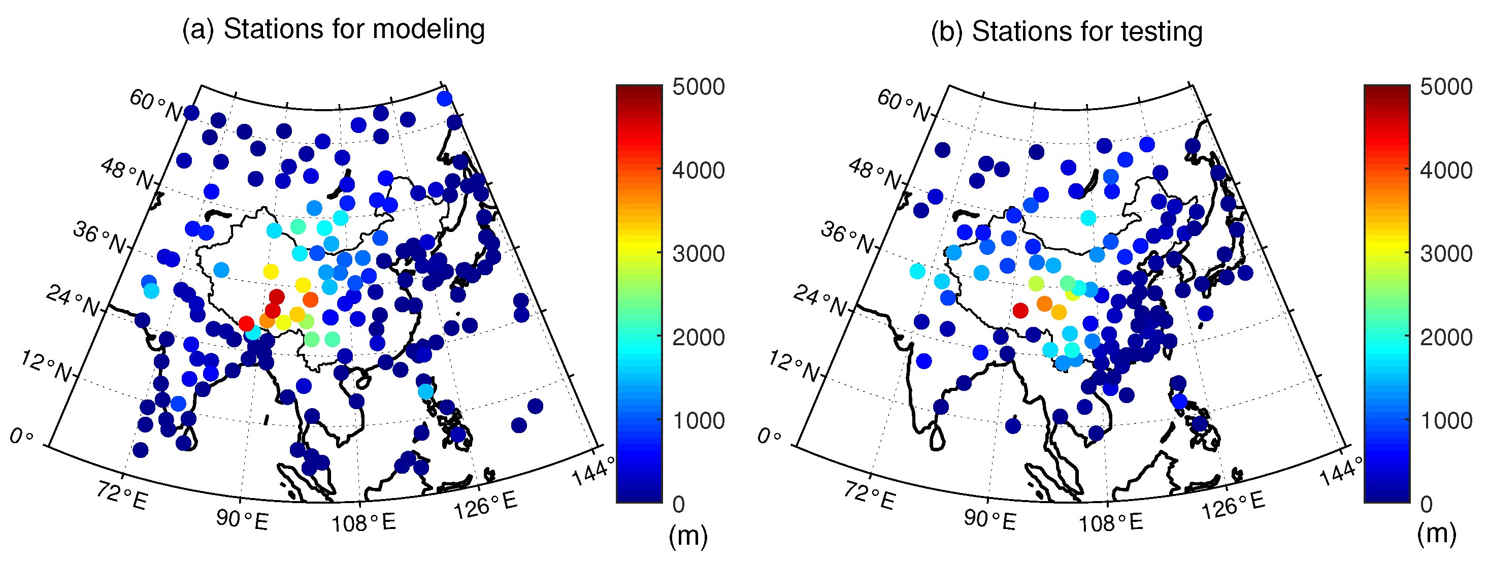
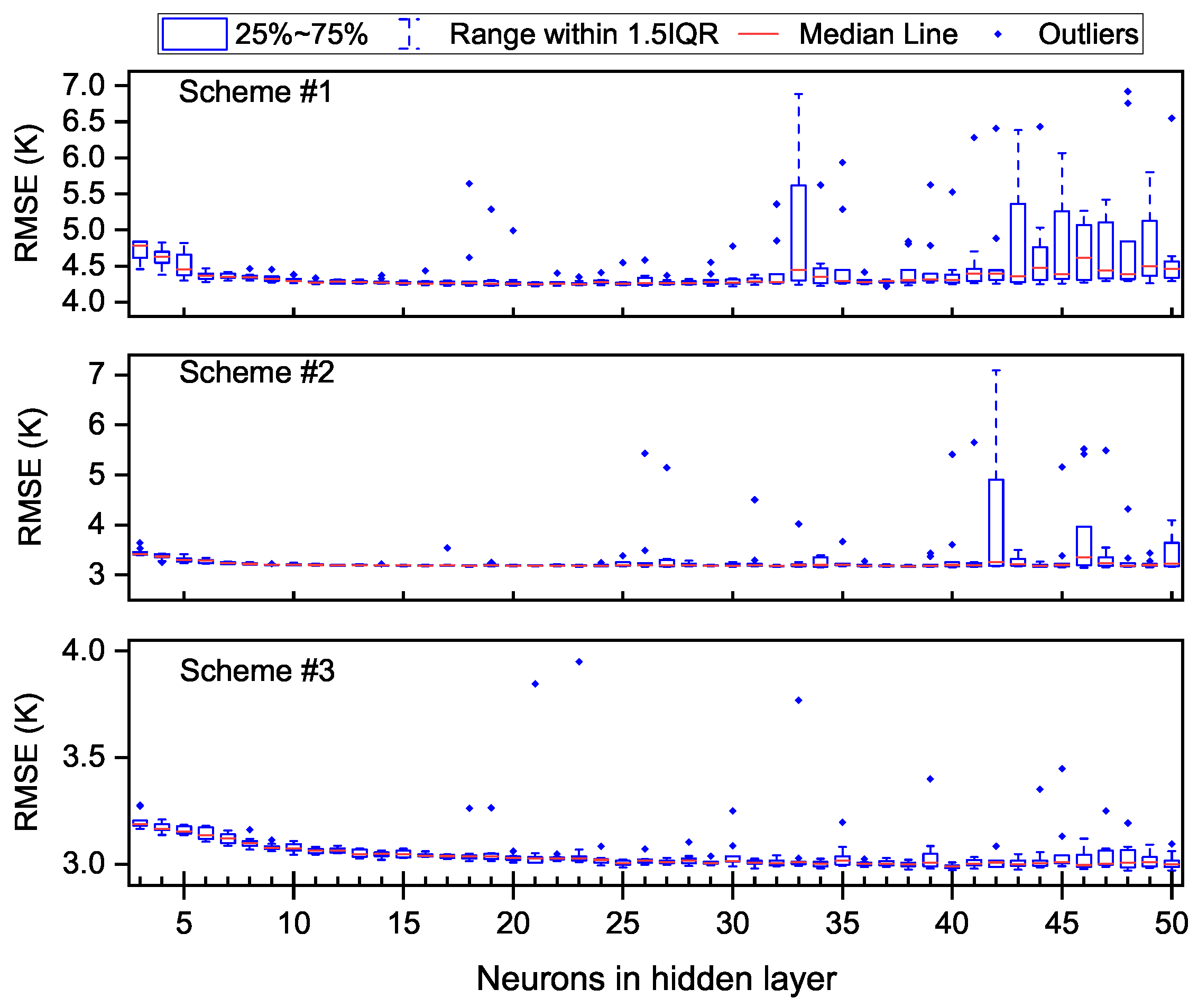
A series of training missions (10 times for each TFNN structure) were carried out, and their generalization performances were discussed. The accuracy of each training mission was evaluated with a total of 113,866 atmospheric profiles measured from 2014 to 2015 at 119 radionsonde stations (see Figure 3); the MBEs and RMSEs of each modeling scheme are shown in Figure 4 and Figure 5.

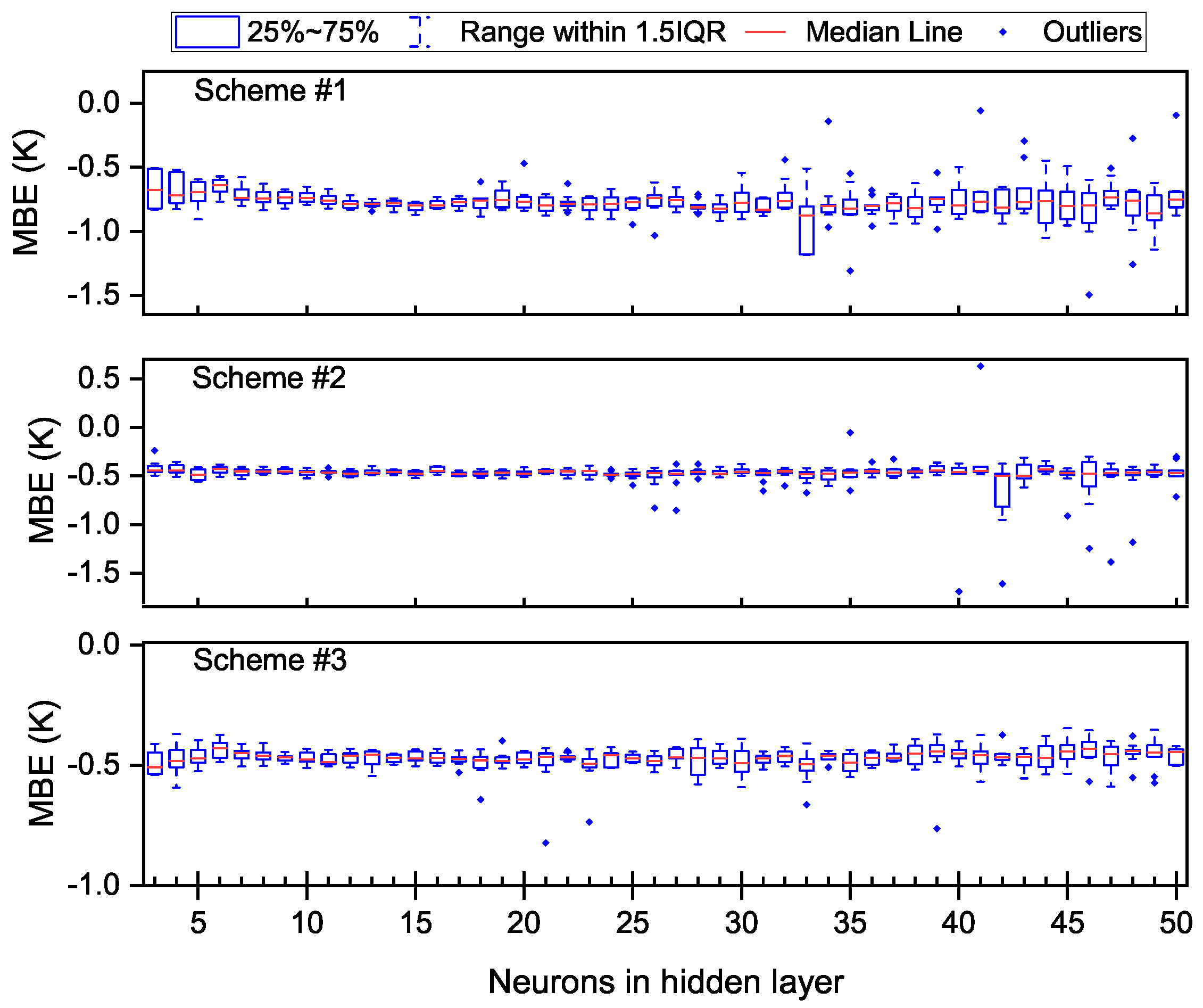
From Figure 4 and Figure 5, one can see that the fluctuation of MBEs and RMSEs increased with the increasing number of neurons in the hidden layer. In terms of MBEs, the MBEs of different TFNN structures were almost always less than 0 K; the reason for this may be that the dataset for modeling ran from 2001 to 2013 but the interannual variation of $T_m$ was not taken into account. Outliers could be found for all of the three modeling schemes when $N_{hid}$ was larger than 16; in particular, scheme #1 and scheme #2 had outliers larger than 0 K when the $N_{hid}$ was larger than 40. Larger negative biases are also common in all modeling schemes when there are more neurons. In the aspect of RMSEs, the largest RMSE of each modeling scheme even reached 7.0 K, 6.5 K and 4.0 K, respectively, while the minimum RMSE always remained at a low level regardless of the neural network structure. Another phenomenon regarding RMSE was that when $N_{hid}$ was smaller than 10, the RMSE decreased as the $N_{hid}$ increased, especially for scheme #1 and scheme #3.

Such large differences in model accuracy between different TFNNs made it risky to choose a specific training result as the final parameter of a $T_m$ model; the overall negative biases of most TFNNs in the estimation of $T_m$ also negatively impacted the utility of the model. Therefore, some measures should be taken into account to improve the generalization performance of TFNN models and eliminate the bias in $T_m$ estimation caused by the interannual variation of $T_m$.

4.2. Strengthening the Generalization Performance of TFNN Models with Ensemble Learning

The training samples of each training mission (which overlapped with each other) and the initial weights were different, and thus the performance of each TFNN was different. If only one individual TFNN were used as the final model, that might lead to poor generalization performance due to poor selection; combining multiple TFNNs is expected to effectively reduce this risk. As the training missions were independent of each other, we adopted the simple averaging method to combine the individual TFNNs, as follows:

$$T_m=\frac{1}{N_{ens}}\sum _{k=1}^{N_{ens}}{T}_{m0}^k$$

(24)

where $T_{m0}^k$ is the $T_m$ value calculated by the k-th TFNN. However, some experiments were required to determine the optimal ensemble size ($N_{ens}$) to ensure the generalization performance of models after combination. From the perspective of bias-variance decomposition, ensemble learning (bagging, for example) mainly focuses on reducing variance, so attention was mainly paid to the RMSEs of models with different ensemble sizes. 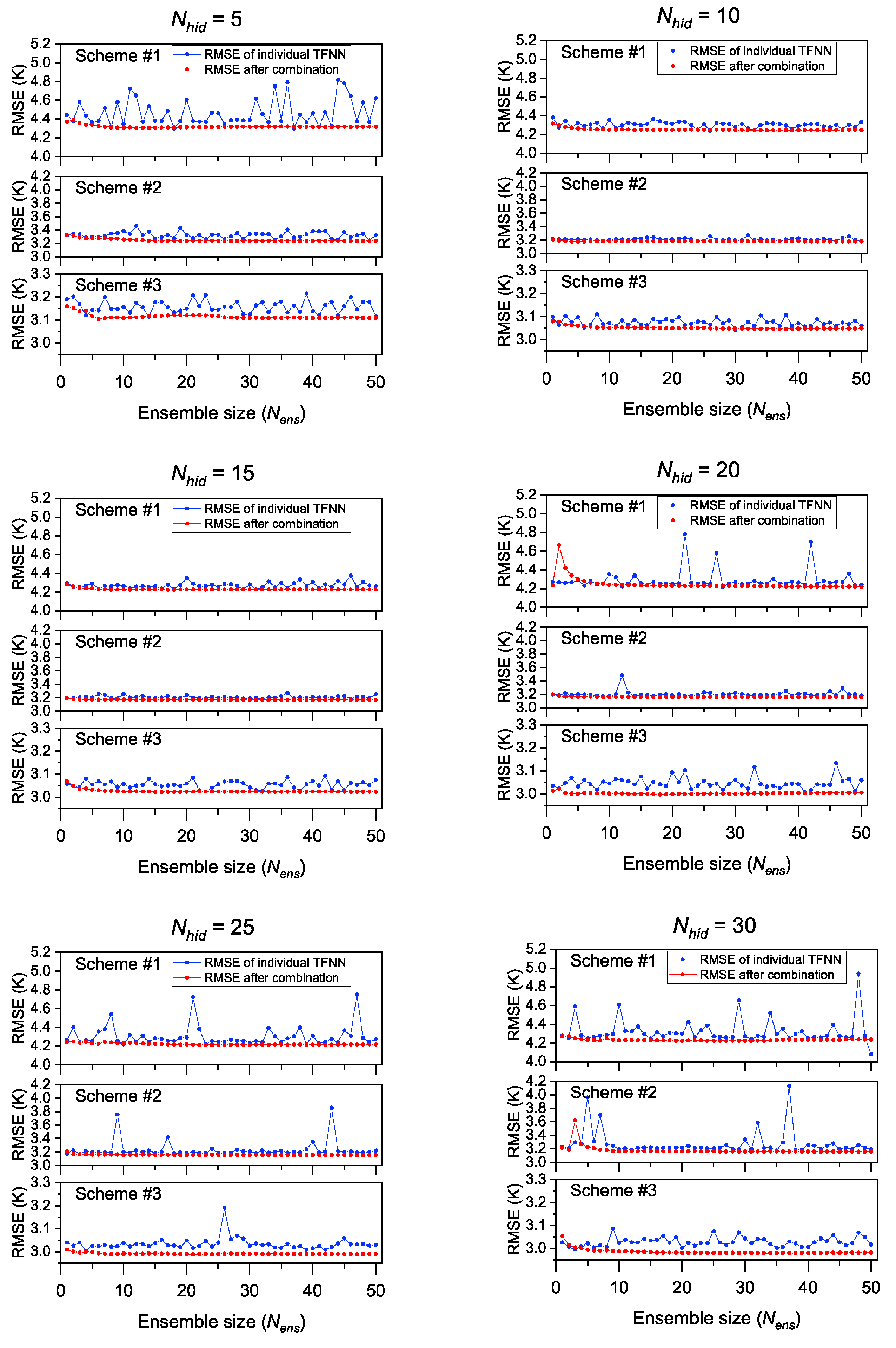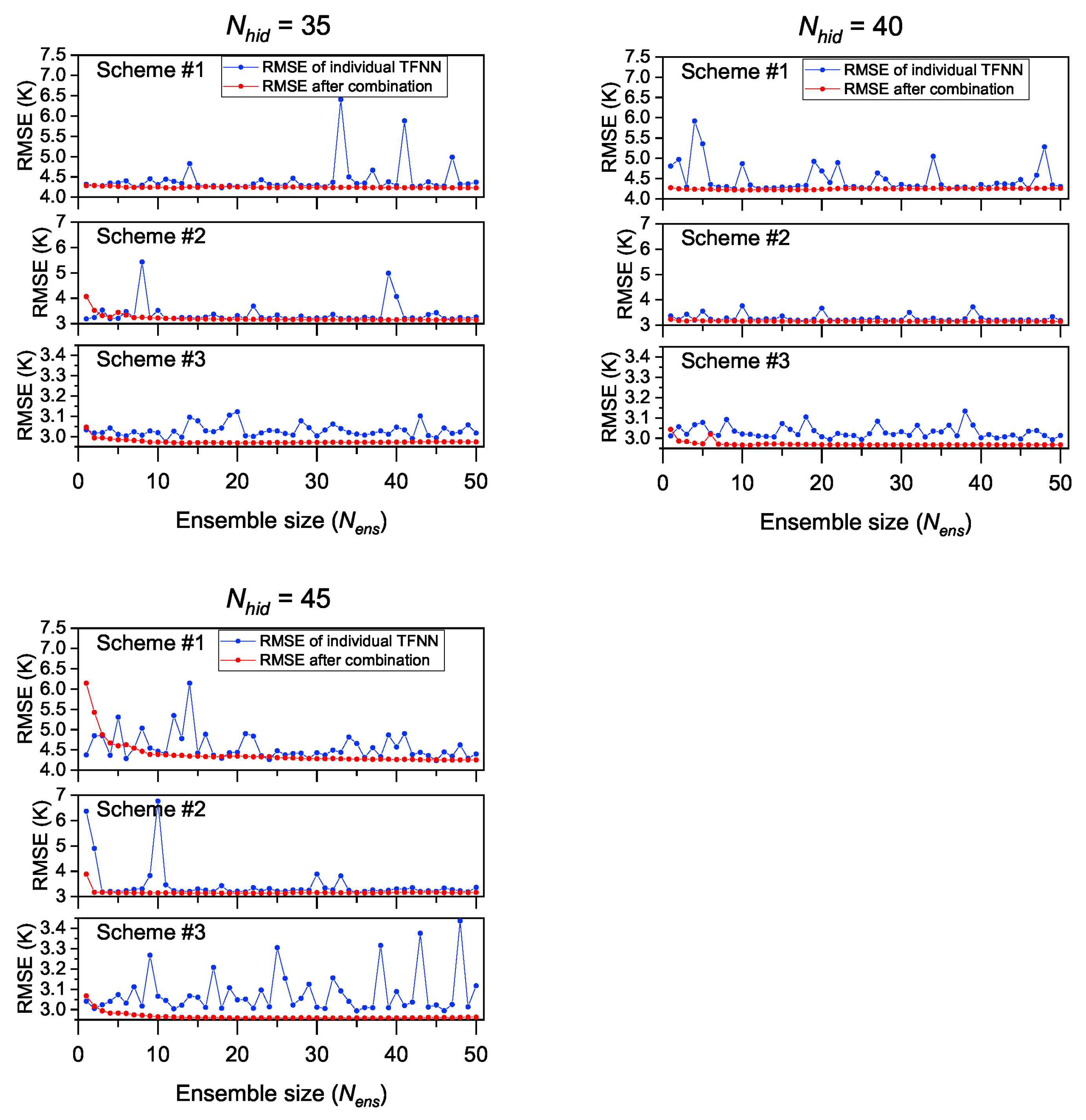Figure 6 and Figure 7 show the RMSEs of models with different ensemble size ($N_{ens}$) when $N_{hid}=5,10,15,20,25,30,35,40,45$.

As can be seen from Figure 6 and Figure 7, the generalization performances of different TFNNs were quite different from each other, especially when there were more neurons in the hidden layer, which is consistent with the results verified in Section 4.1. However, general improvements in RMSE were found for each modeling scheme when we combined multiple individual TFNNs; the accuracy of the results after combination showed remarkable improvement compared with individual TFNNs in most cases.

From the perspective of each modeling scheme, there was no obvious abnormal RMSE for scheme #1 when the $N_{hid}$ was 10 or 15, and the RMSE values were generally between 4.2 K and 4.4 K, but great fluctuations could be found when $N_{hid}$ was larger than 20, with the maximal RMSE even reaching 4.9 K to 6.5 K when the $N_{hid}$ was between 20 and 45. When $N_{hid}$ was 5, the fluctuation of RMSE was also obvious, ranging from 4.3 K to 4.8 K. However, the uncertainties in $T_m$ calculation disappeared after combination, even when the $N_{hid}$ was larger than 20. Regarding scheme #2, a similar situation to scheme #1 can be observed, in that the RMSEs were between 3.20 K and 3.25 K when the $N_{hid}$ was 10 or 15, but larger RMSEs were shown when the $N_{hid}$ was larger than 20; particularly large RMSE values could be found when $N_{hid}$ was 35 or 45, with maximal values of 5.5 K and 6.8 K, respectively. When the $N_{hid}$ was 5, the fluctuation of RMSEs was not drastic, but their values were larger than those in case of $N_{hid}$ = 10. The improvement of the generalization performance of scheme #2 using ensemble learning was also significant, especially when $N_{hid}$ was larger than 20. However, scheme #3 performed differently to scheme #1 and scheme #2. Only when $N_{hid}$ was very large (for example, $N_{hid}$ = 45) did the abnormal RMSEs increase significantly. In other times, the differences of RMSEs between individual TFNNs was not obvious, fluctuating by approximate 0.1 K. By combining different TFNNs, the influence of TFNN with poor generalization performance on $T_m$ calculation was also effectively eliminated. We can also see from Figure 6 and Figure 7 that the ensemble size did not need to be set to be overly large: a $N_{ens}$ of about 10 could achieve the effect of improving the generalization performance of the TFNN models.

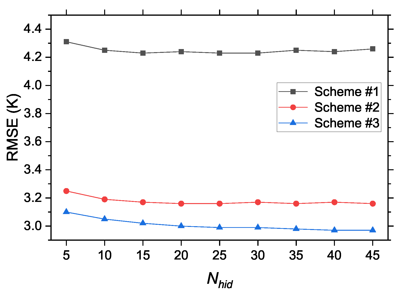
In general, the generalization performances of individual TFNNs fluctuated, and with the increase of $N_{hid}$, the generalization performance changed drastically. The uncertainty of the generalization performance could be significantly reduced by combining different TFNNs, but a balance should be struck between improving model accuracy and reducing uncertainty risk. We compared the combination results of different modeling schemes when the number of neurons in the hidden layer was 5 to 45; the results are shown in Figure 8.

One can see from Figure 8 that the RMSE of each modeling scheme after combination decreased with the increasing $N_{hid}$, but the improvement in model accuracy was not significant when the $N_{hid}$ was large; e.g., it only improved by approximately 0.05 K for scheme #1, 0.1 K for scheme #2 and 0.15 K for scheme #3 when $N_{hid}$ ranged from 5 to 45. This improvement was insignificant, but a risk of overfitting may occur due to the increasing complexity of the neural network structure. From the analysis of Figure 6 and Figure 7, little difference can be seen in terms of the generalization performance if different individual TFNNs when $N_{hid}$ was 10 or 15, and the accuracy of results after combination was only slightly poorer than when there were more neurons in the hidden layer.

4.3. The Impact of Interannual Variations of $T_m$

The interannual variation trend of $T_m$ has been demonstrated in many previous studies [4,23,36,42]. It has been shown in the literature [42] that $T_m$ has an increasing trend over the long term on a global scale and increases by about 0.24 K per decade in the north temperate zone, while the radiosonde stations used for modeling in this study are mainly distributed at latitudes between ${10}^{\circ }$ N and ${60}^{\circ }$ N. 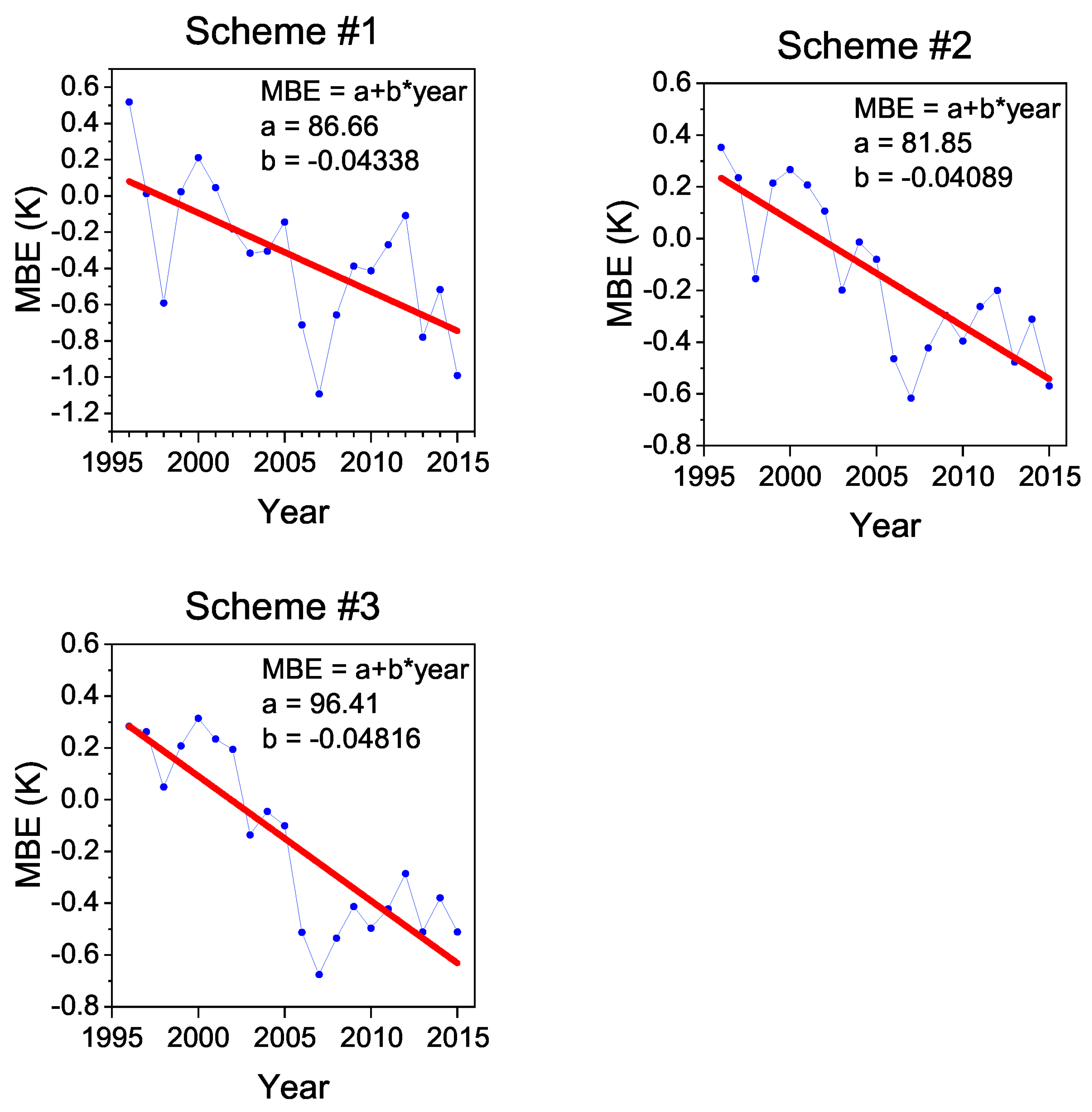It is necessary to discuss the biases of new models caused by long-term trends of $T_m$, since the data for modeling in this study were all from 2001 to 2013. The yearly biases of the three modeling schemes from 1996 to 2015 are shown in Figure 9.

From Figure 9, an approximately linear trend in bias can be found for all the modeling schemes: their decline rates are −0.043 K/year, −0.041 K/year and −0.048 K/year, respectively. There is an obvious decreasing trend in $T_m$ biases calculated with neural network models, which presents a challenge for the generalization performance of new models.

However, the neural networks are actually much better at interpolation than extrapolation; thus, the $doy$ was considered to be one of the input variables to simulate the periodic variation characteristics of $T_m$ within the year, but parameters of interannual variation of $T_m$ were not included in new models. The negative bias of $T_m$ estimation caused by long-term trends of $T_m$ cannot be ignored, so an external correction to new models was considered in this study:

$$T_m=\frac{1}{N_{ens}}\sum _{k=1}^{N_{ens}}{T}_{m0}^k-(a+b·year)$$

(25)

where $T_{m0}^k$ is the $T_m$ value calculated by an individual TFNN, $N_{ens}$ is the ensemble size and a and b are the correction parameters for interannual bias, which can be seen in Figure 9.

4.4. Discussion

The ANN technique shows a powerful capability to capture the spatiotemporal variation characteristics of $T_m$ in this study. In this section, thousands of experiments showed that the robustness of TFNN models was good enough, but uncertain risks in model accuracy were shown when the model was validated with data that were not involved in modeling, which is expressed as the generalization performance of TFNN fluctuating drastically when its structure changes. In previous studies, some researchers tried to demonstrate the feasibility of the neural network technique in $T_m$ modeling, but they only used the results of a certain training mission as the final model parameter; the generalization performance of these models were not sufficiently considered, and the models probably incur great uncertainty risks when they are put to actual use. The ensemble learning method was proposed in this study to make up for this defect, and the test results showed that the generalization performance of new models was effectively enhanced. Moreover, the significant negative bias in the $T_m$ estimation with new models caused by the interannual variation of $T_m$ cannot be ignored, and thus an external correction was made to the results of TFNN models after combination.

We set the ensemble size of TFNN models as 10 and the number of hidden layer neurons as 10 or 15 and made a simple external correction to the results after combination. The three models developed in this study are named the NMFTm model (corresponding to modeling scheme #1; no meteorological factor is required), SMFTm model (corresponding to modeling scheme #2; a single meteorological factor is needed) and MMFTm model (corresponding to modeling scheme #3; multiple meteorological factors are needed), respectively, and were able to meet the requirements of $T_m$ calculation under different application conditions.

5. Model Accuracies Compared with Other Published Models

In order to examine the accuracies of new models, comparisons between new models and several representative published models are presented in this section. These models are the GTm_R model, Bevis model, TVGG model, NN-I model and GTm-I/PTm-I model. There are some differences in the calculation of $T_m$ with these models:

• No meteorological factor is required for the GTm_R model and NMFTm model;
• Only $T_s$ is required for the Bevis model, GTm-I model, TVGG model and SMFTm model;
• Both $T_s$ and $e_s$ are necessary for the PTm-I model and MMFTm model.

Measured profiles of 119 radiosonde stations were utilized, and the mean bias error (MBE) and root-mean-square error (RMSE) were used to evaluate the model accuracy. The $N_{hid}$ values of the new models corresponding to the results presented in this section were all 10.

5.1. Accuracies for All Testing Samples from 2016 to 2018

We first tested the performance of different models with a total of 191,812 radiosonde profiles measured from 2016 to 2018, as with the data used in Section 4; these data were also independently and identically distributed to the dataset for modeling. The MBE and RMSE for different models are shown in

Table 3. Statistics of $T_m$ estimates for different models tested by radiosonde data from 2016 to 2018.

Statistics	GTm_R	Bevis	TVGG	NN-I	GTm-I	PTm-I	NMFTm	SMFTm	MMFTm
MBE (K)	−1.30	−0.39	−1.85	−0.65	−1.60	−1.36	−0.01	0.05	0.11
MS_MBE (K)	−1.26	−0.39	−1.98	−0.62	−1.84	−1.51	0.08	0.12	0.16
RMSE (K)	4.33	4.33	3.75	3.46	4.09	3.71	4.15	3.14	2.96
MS_RMSE (K)	4.09	4.19	3.64	3.31	3.98	3.58	3.96	3.03	2.87

; the MBE and RMSE of each station (named as S_MBE and S_RMSE) are also calculated and their respective mean values (named as MS_MBE and MS_RMSE) are shown in Table 3.

From Table 3, one can see that the GTm_R model, TVGG model and GTm-I/PTm-I model showed much larger biases (both in MBE and MS_MBE) than the Bevis model, NN-I model and new models. The reason for this is that the GTm_R model, TVGG model and GTm-I/PTm-I model were all developed using reanalysis data (ERA-Interim), while the others were developed using data collected by radiosounding. As mentioned in Section 2.2, data collected via radiosounding are closest to the actual situation and undoubtedly the most appropriate dataset for developing a regional $T_m$ model that is close to reality. The Bevis model is a classic $T_m$ model, and its bias is the smallest of all the published models. The biases of the SMFTm model and MMFTm model with enhanced generalization capability were much better than the NN-I model in terms of MBE and MS_MBE. The NMFTm model showed the largest bias of the new models, but great improvement can be seen compared with the GTm_R model. It is worth mentioning that the published models listed in this study were all developed with historical datasets, but the interannual or interdecadal variation tendency of $T_m$ was not taken into account; this may be another important reason for the large negative biases of these models when verified with the data from 2016 to 2018.

In terms of RMSE, larger RMSEs can be seen for the GTm_R model and Bevis model. GTm-I model performed a little better because it is a grid model and combines the modeling ideas of the GTm_R model and the Bevis model; that is, the Bevis formula is first used for modeling and then the annual and semi-annual variation characteristics of residuals caused by the Bevis formula are simulated. The performance of the PTm-I model improved by 9% in RMSE (0.4 K) compared to the GTm-I model as the surface water vapor pressure was taken into account in the development of the PTm-I model; it can be seen that the introduction of water vapor pressure into $T_m$ modeling is very beneficial to the improvement of model accuracy. The TVGG model follows a similar modeling approach to the GTm-I model, but it is further optimized; that is, the coefficients of the Bevis formula at each grid are calculated rather than regressing on a global scale, and the resulting residuals are finally simulated with a trigonometric function. An improvement of approximately 9% (0.3 K) in RMSE could be found for the TVGG model compared to the GTm-I model; thus, we only consider TVGG model in the following analysis since their modeling principles are basically the same.

The NN-I model uses the the coefficients of the GPT2w model to describe the periodic variations of $T_m$ and uses neural network as modeling tool, and it showed the best accuracy on a global scale of all the published models listed in this study; it can also be seen from Table 3 that its RMSE (MS_RMSE) within the study area was far smaller than the other published models. However, the NN-I model also has drawbacks; i.e., it relies on the $T_m$ values derived from the GPT2w model and it is developed for global users, but only one set of weight and bias values after a certain training mission is provided, and its accuracy in a specific region has not been verified yet. The complexity of the model can be reduced and the generalization performance can be strengthened by optimizing the modeling process. The new models were all developed based upon the dataset within the study area, and their generalization performances were strengthened via the ensemble learning method. It can be seen from Table 3 that the RMSE of the SMFTm model was 9.3% better than the NN-I model, and when we further incorporated the water vapor pressure into modeling, the MMFTm model outperformed the NN-I model by 14.5% in terms of RMSE, and the improvement in accuracy of the MMFTm model compared with SMFTm model was also quite obvious (0.18 K for RMSE and 0.16 K for MS_RMSE). Although the accuracy of the NMFTm model was not greatly improved compared with the GTm_R model (they both correspond to the category of NMF models), it has the advantage of being simple and universal for the users within the study area.

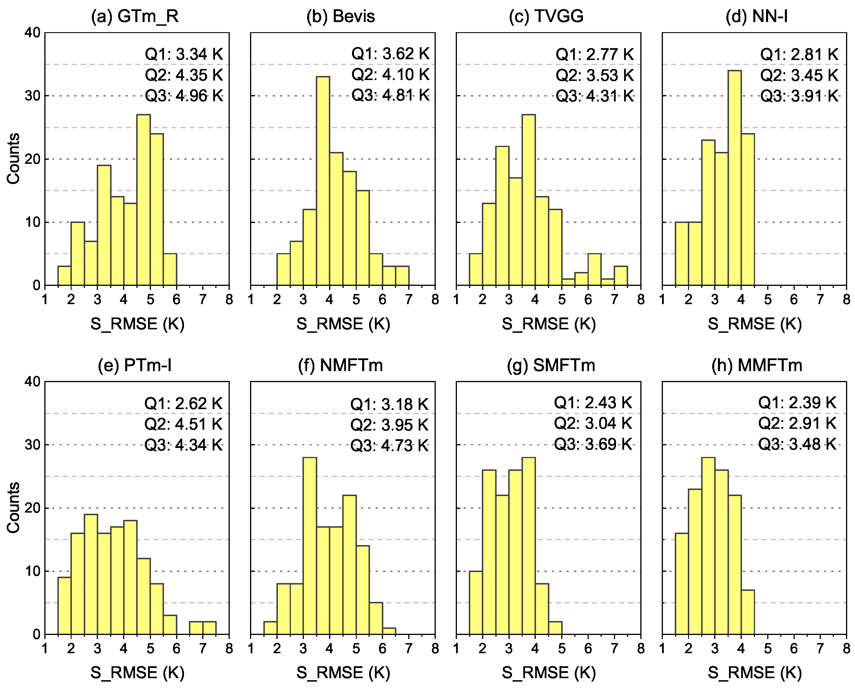
5.2. Accuracies Tested by Single Testing Stations

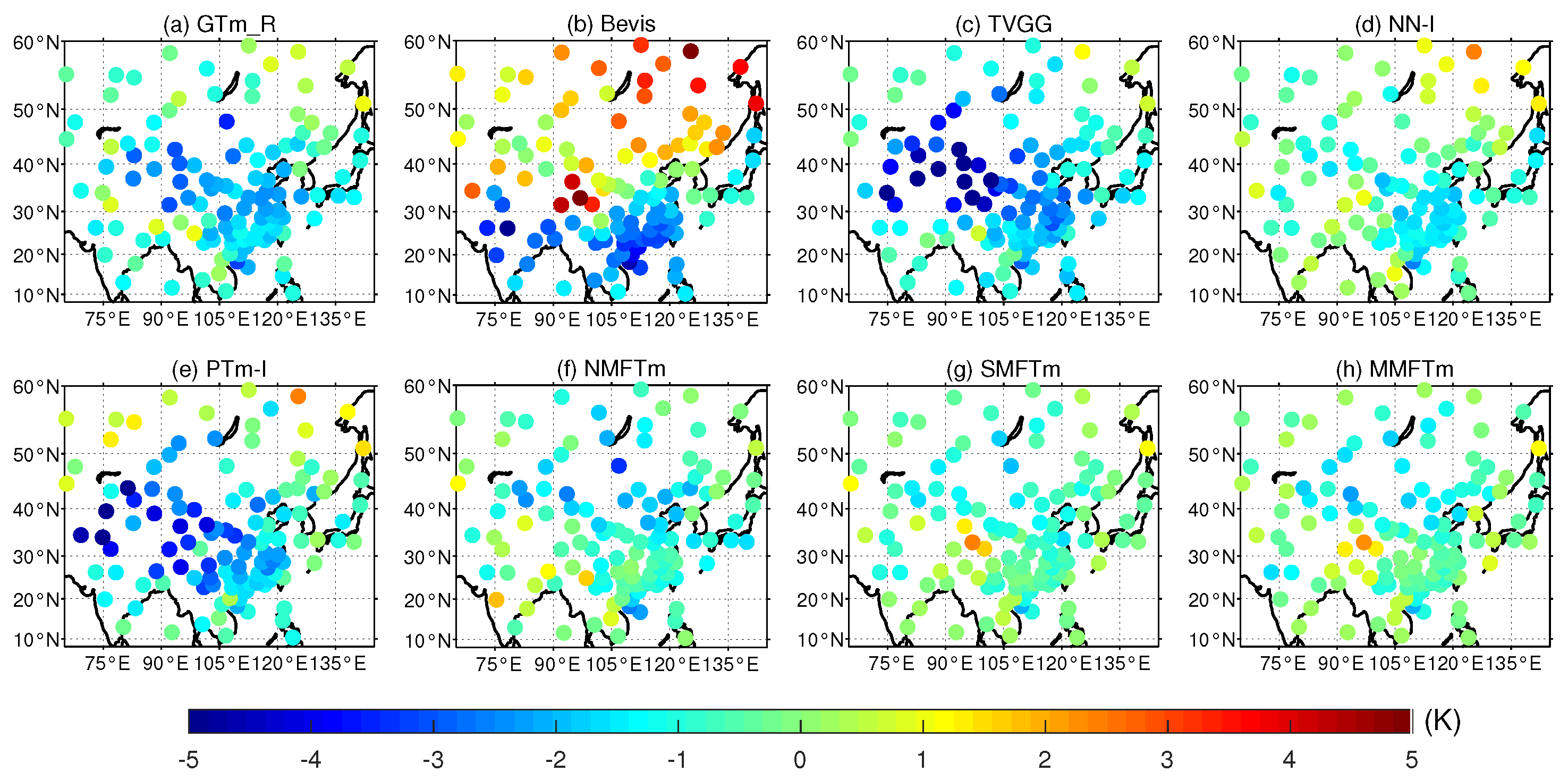
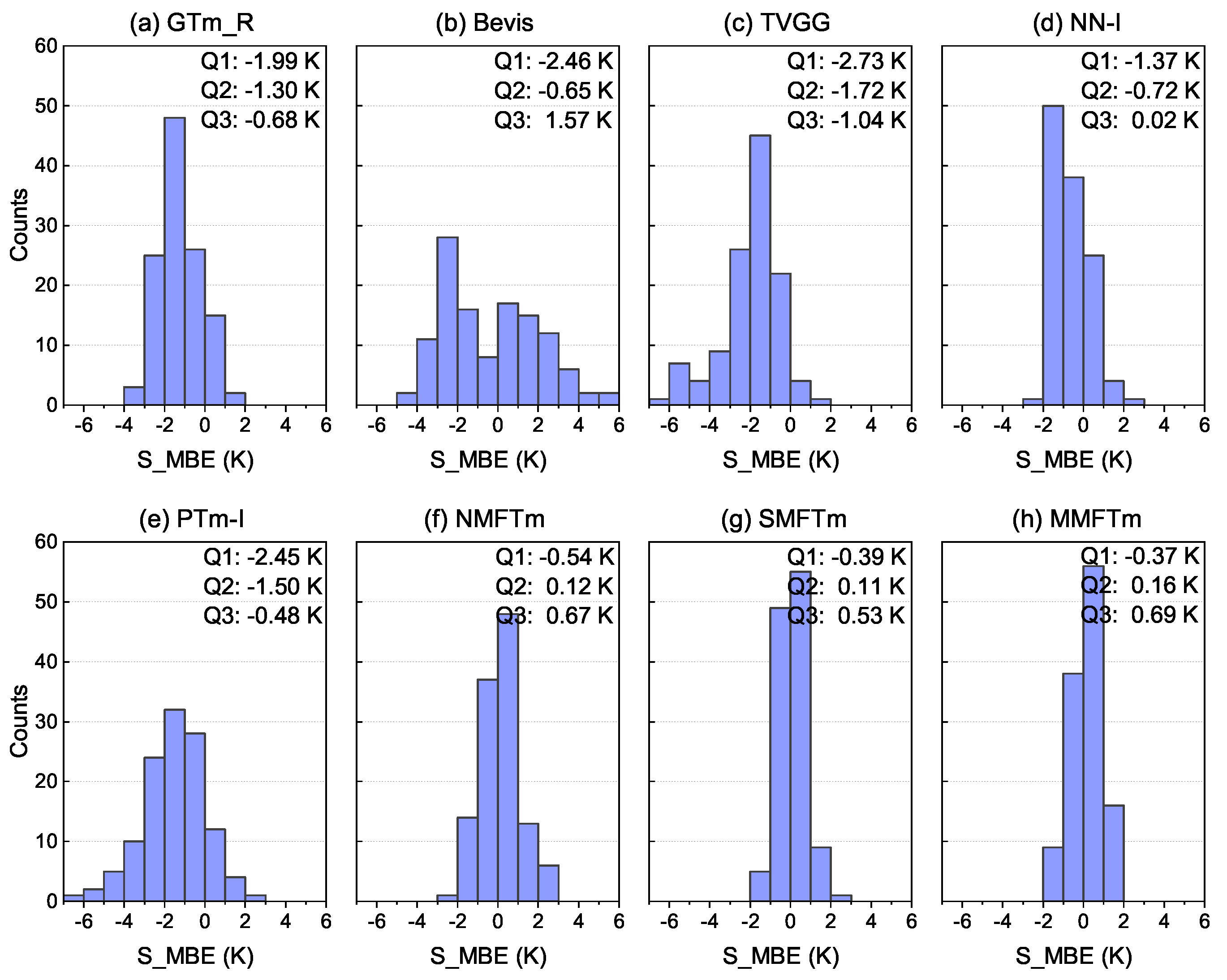
We further compared the performance of different models at each single testing station. The distribution and statistics of S_MBE and S_RMSE for different models can be seen in Figure 10, Figure 11, Figure 12 and Figure 13.

Figure 10 and Figure 11 show that the TVGG model and PTm-I model exhibited significantly larger systemic negative biases than other competing models; both of them had a large proportion of S_MBEs over −1.0 K, and these testing stations with larger biases were mainly distributed in the western and northwestern regions of China. The GTm_R model also showed a systemic negative bias, but its S_MBEs mainly ranged between −2.5 K and 0.5 K, and the bias was mainly contributed by stations in the northern region of China. Although the S_MBEs of the Bevis model were evenly distributed from −4.0 K to 4.0 K, the absolute S_MBEs over 2.0 K accounted for more than half of the total and the biases of stations distributed in the study area were distinctly different; that is, stations located at latitude below ${30}^{\circ }$ N had negative biases while the majority of stations located further north had large positive biases, which indicates that the Bevis model is not applicable to China and adjacent areas. The S_MBEs of neural network-based models (including NN-I model and new models) were almost concentrated in the range from −2.0 K to 1.0 K and were therefore better than those of other competing models, but slight systemic negative biases could be found for the NN-I model. Both the SMFTm model and MMFTm model outperformed the NN-I model: their S_MBEs in most testing stations were between −1.0 K and 1.0 K, and the Q1 (25th percentile), Q2 (50th percentile) and Q3 (75th percentile) values were closer to 0 K than other models. Large negative biases could be found for the NMFTm model in the northern part of the study area, but overall, it performed better than the GTm_R model, Bevis model, TVGG model and PTm-I model in terms of S_MBE.

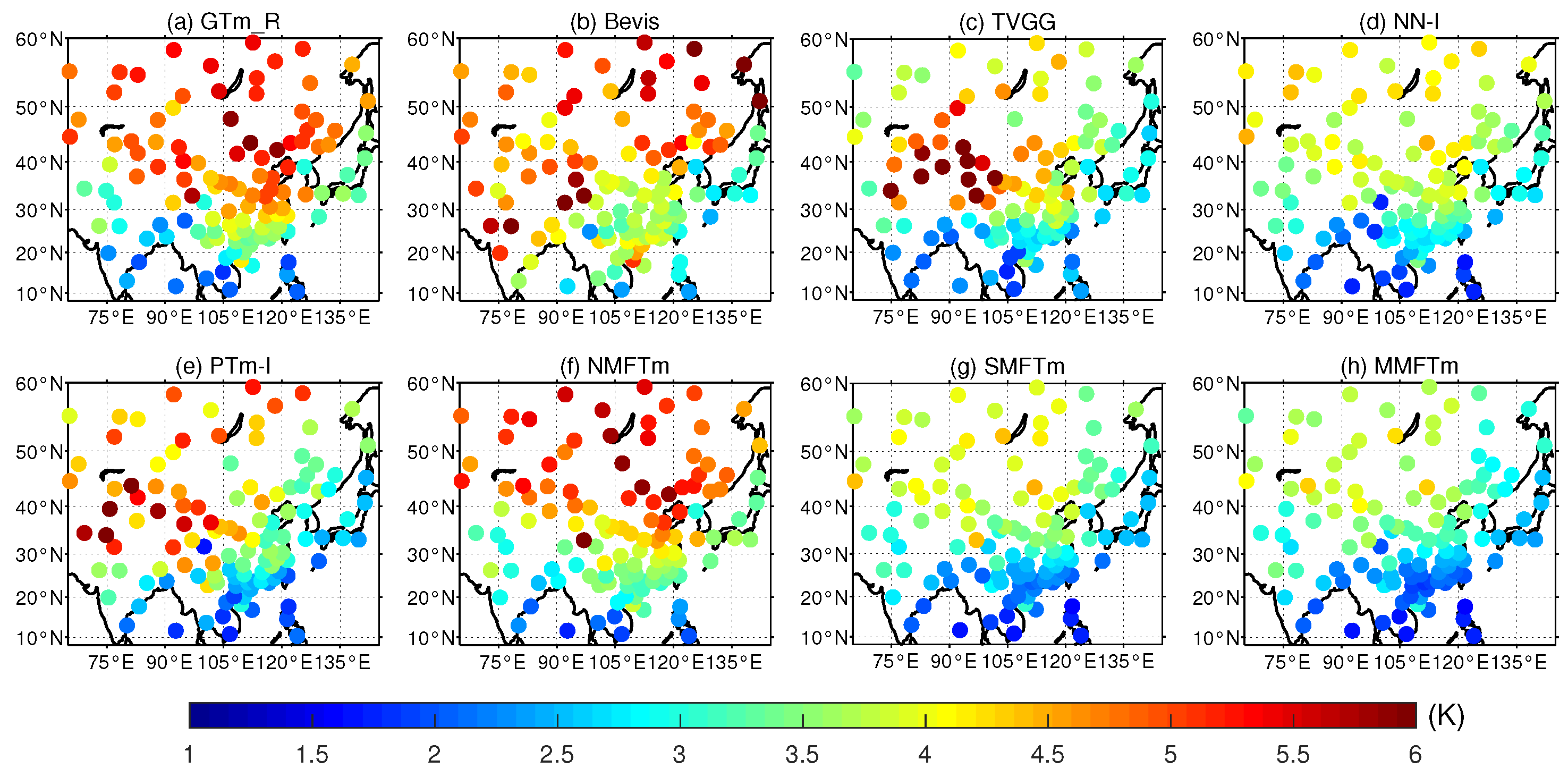
With regard to S_RMSE, one can see from Figure 12 and Figure 13 that both the GTm_R model and NMFTm model showed a very large S_RMSE in the northern part of the study area. Although the GTm_R model is a grid model with a spatial resolution of $1^{\circ }\times 1^{\circ }$, its advantage in accuracy over neural network-based NMFTm model is not obvious; it did not even match the NMFTm model in many places, such as at latitudes between ${30}^{\circ }$ N and ${40}^{\circ }$ N. It is worth noting that both the GTm_R model and NMFTm model correspond to the category of NMF models, and their S_RMSEs in most testing stations were in the range between 4.0 K and 6.0 K; the error of converting GNSS–ZWD to PWV caused by these models cannot be ignored in practice. The Bevis model, although a very classic SMF model, does not take into account the impact of geographic location on model accuracy, and thus its accuracy in the northern part of the study area was not significantly improved compared with NMF models. The TVGG model and PTm-I model are both grid SMF models, and the impact of geographic location differences were considered, meaning that they outperformed tge Bevis model in most areas; however, a significantly large RMSE could still be found in the northwestern region of China. There are two main reasons for this: (a) the data source for modeling was reanalysis data derived from the assimilation system, (b) the impact of height differences between the target location and grid points was not taken into account. The flaws of the GTm_R model, Bevis model, TVGG model and PTm-I model were clearly overcome by the neural network-based SMF models including the NN-I model, SMFTm model and MMFTm model. From Figure 12, one can see that the S_RMSEs of stations at the latitudes from ${40}^{\circ }$ N to ${60}^{\circ }$ N and stations in the southeastern part of China from SMFTm model and MMFTm model were smaller than those from the NN-I model. From Figure 13, much smaller Q1 values and Q3 values could be seen for the SMFTm model and MMFTm model compared with other competing models.

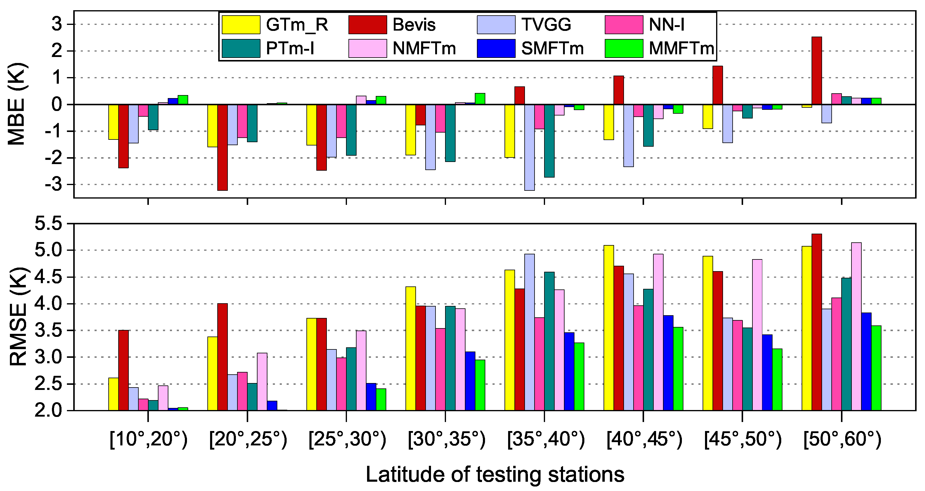
5.3. Accuracies at Different Latitudes

The solar radiation intensity at different latitudes was inconsistent, which was the most important reason for the regional differences of $T_m$, and many studies have shown the strong correlation between $T_m$ and geographic location (mainly latitude). We sorted the testing dataset into eight groups, each with a latitude span of $5^{\circ }$. The MBE and RMSE of each group are shown in Figure 14.

Figure 14 shows that the GTm_R model, TVGG model and PTm-I model had remarkable negative biases at almost all the latitude ranges, while the Bevis model showed great negative bias at stations located south of ${35}^{\circ }$ N, but a marked positive bias could be seen at stations further north, which corresponds to the results shown in Figure 10. The neural network-based models, however, showed much smaller biases at all the latitude ranges; a large negative bias of the NN-I model could be seen mainly at the latitude range of [${20}^{\circ }$ N, ${40}^{\circ }$ N], and the NMFTm model showed a larger negative bias at the latitude from ${35}^{\circ }$ N to ${45}^{\circ }$ N. The SMFTm model and MMFTm model performed best in terms of the MBE.

In terms of RMSE, RMSE values were smaller at low latitudes, but a larger RMSE could be found at higher latitudes for all the competing models. The Bevis model showed the largest RMSE at low latitudes, and its performance was even poorer than the GTm_R model and NMFTm model; it even failed to show an advantage in accuracy over the NMF model as latitude increased. Other SMF models except for the PTm-I model showed much smaller RMSEs, but the performance of PTm-I model was still inferior to the TVGG model, NN-I model and SMFTm model in almost all the latitude ranges, even though it took the surface water vapor pressure into account. The performances of the TVGG model at different latitude ranges were different: its RMSE first increased and then decreased with increasing latitude. Improvements in RMSE could be found for the SMFTm model at all the latitude ranges compared with the NN-I model. The RMSE of the MMFTm model was always the smallest if all the competing models, and a significant improvement could also be seen compared with the SMFTm model.

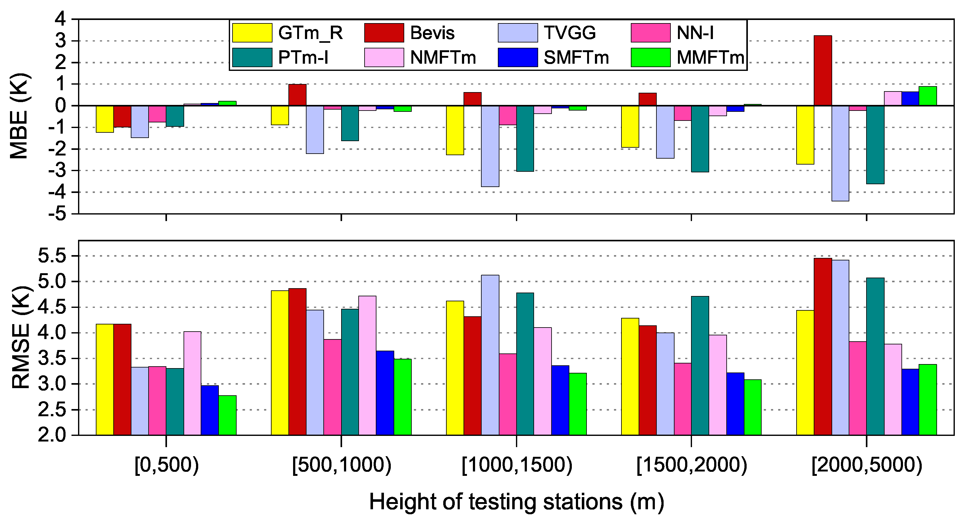
5.4. Accuracies at Different Heights

The height (height above sea level) of the station is considered as an input variable in the development of new models. We compared the MBE and RMSE at different height ranges for different competing models. The testing dataset was sorted into five groups according to height: i.e., below 500 m, 500–1000, 1000–1500, 1500–2000 and above 2000 m. The results are shown in Figure 15.

From Figure 15, very large biases could be found at the heights over 500 m for TVGG model and PTm-I model, since they do not take the height as input variable. GTm_R model reduces the bias of $T_m$ estimation caused by the height differences between target location and grid points, but remarkable bias can still be found at the heights over 1000 m. Bevis model performs well at the heights below 2000 m in terms of MBE, while significant positive biases could be found at the heights over 2000 m. NN-I model actually takes into account the impact of height differences by setting a constant lapse rate of −5.1 K/km [17], the results show that its bias at each height range is also very small. The new models, however, all take the height above sea level as one of the input variables, and their biases are very small at all the height ranges.

In the aspect of RMSE, the largest RMSE of GTm_R model can be found at the heights from 500 m to 1000 m, the performance of NMFTm model is similar to that of GTm_R model, but slight improvement can be found at the heights over 1000 m. As TVGG model and PTm-I model do not incorporate the height into the model, their RMSEs are closer to those of neural network-based models when the height is less than 500 m, but with the height increases, their performance are even poorer than those of NMF models. Bevis model performs the poorest at almost all the height ranges, since Bevis model doesn’t contain any information about the geographic location or terrain. Significant improvement is shown for SMFTm model and MMFTm model at the heights below 500 m and heights over 2000 m compared with NN-I model, but their advantages are not obvious at the height from 500 m to 2000 m. MMFTm model has marked advantages over SMFTm model at low altitudes, but this accuracy advantage disappears at the heights over 2000 m.

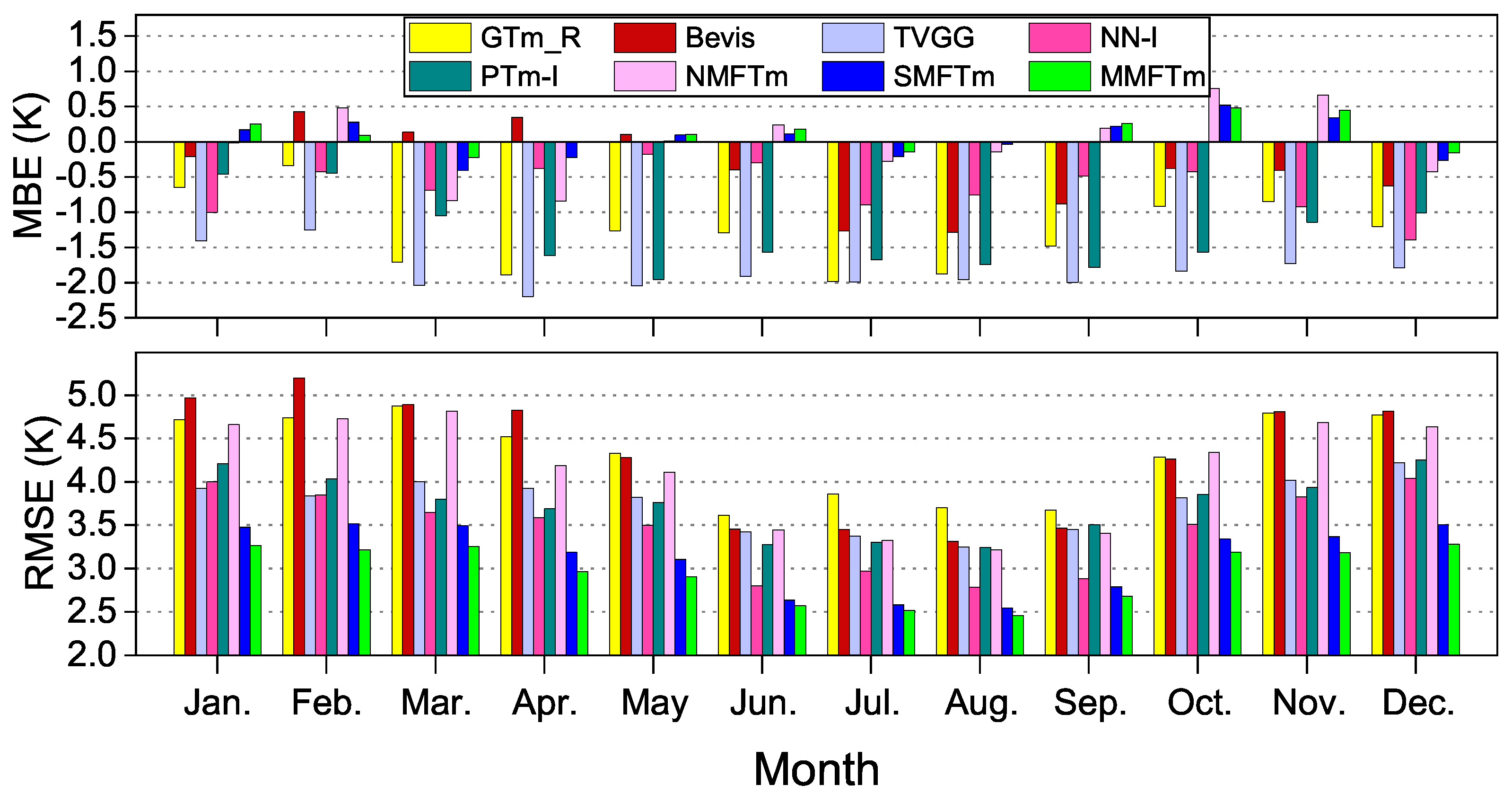
5.5. Accuracies in Different Months

The seasonal accuracies of different models were also examined in this study. We calculated the monthly MBE and RMSE for different models with radiosonde data from 2016 to 2018, the results are shown in Figure 16.

From Figure 16, much larger biases can be found during spring and summer months than those in winter for almost all the competing models. It can be seen that the biases of NMFTm model are much smaller than those of GTm_R model in summer and autumn months (from May to November), but they behave similarly in other months. Unlike the other models, Bevis model shows small positive biases in the first half of the year, and significant negative biases in other months. TVGG model always shows the largest negative biases throughout the year, PTm-I model is slightly improved, but it can still be seen that the negative biases are obvious throughout the year except for winter months. The neural network-based SMF models behave similarly and much smaller negative biases can be found for them throughout the year compared with most of other competing models. The improvements of SMFTm model and MMFTm model are significant compared with NN-I model in winter months.

On the RMSE side, one can see the opposite pattern of seasonal variation characteristic from the MBEs case for most of the competing models i.e., RMSEs are much smaller in summer months than those in other months. The reason is that the variation characteristic of $T_m$ during the summer is easier to be simulated than that in winter months [26,29]. The RMSEs of both GTm_R model and NMFTm model are much larger than those of SMF models almost throughout the year, but the RMSEs of NMFTM model are significantly smaller compared with GTm_R model in summer months. In the aspect of SMF models, Bevis model performs the poorest since it doesn’t consider the seasonal variation charateristics of $T_m$, TVGG model and PTm-I model perform similarly because the $doy$ and even $hod$ were taken into account as the input variables, but they both show larger RMSEs than those of neural network-based SMF models. The PTm-I model even failes to perform as well as the TVGG model in some cases, even though the water vapor pressure was taken into account as one of the input variables. NN-I model outperforms TVGG model and PTm-I model throughout the year, particularly during summer months. SMFTm model shows much higher accuracy than NN-I model especially in winter months, the improvement of MMFTm model over SMFTm model is also significant throughout the year. We believe that the water vapor pressure should still be considered as an important input variable in $T_m$ modeling.

5.6. Discussion

From the comparative analysis above, we find that the new models developed in this study showed better performance than other published models under the same application conditions. The NMFTm model presented some improvements over the GTm_R model in almost all aspects, but its greatest advantage lies in its simplicity and utility. The SMFTm model only took $T_s$ as one of the model inputs, but its accuracy in terms of the RMSE improved by 27.5%, 16.3% and 9.3% over the Bevis model, TVGG model and NN-I model, respectively; its advantages could be found not only in the RMSE of single stations, but also at different latitudes and heights, as well as in different months. Both the MMFTm model and PTm-I model considered the surface water vapor pressure as one of the input variables, but the accuracy of MMFTm model was 20.2% better than that of the PTm-I model. Moreover, the MMFTm model showed the best performance of all the competing models from different perspectives.

The variations of $T_m$ are complex and closely related to weather conditions, but its spatiotemporal variation characteristics follow distinct rules that have been described in previous studies. On the global scale, the variation of $T_m$ shows obvious characteristics of latitude distribution and is related to topography and land-sea distribution. In terms of specific regions, $T_m$ in most regions exhibits an evident periodicity of properties, including annual, semiannual and diurnal variation characteristics, which are the basis of $T_m$ modeling. In the analysis presented in this section, significant differences in accuracy are shown for different models, and we think that the reasons for this result can be summarized as follows:

(1).

The data sources for modeling: The GTm_R model, TVGG model and GTm-I/PTm-I model were all developed using reanalysis data, and uncertainties exist in extracting meteorological elements and calculating $T_m$ from reanalysis data, resulting in large biases for these models, which can be seen in many respects from the comparisons above. The Bevis model, NN-I model and new models, however, were all developed using the data collected by sounding balloons; their biases are smaller and the models are closer to the actual situation.

(2).

The surface meteorological elements: The GTm_R model and NMFTm model are NMF models, and their accuracies are not as good as those of other models because the surface meteorological elements are not involved in the model. The performance of the TVGG model was poorer than that of the PTm-I model since the PTm-I model further considers the surface water vapor pressure as one of the inputs. This is also the case for the performance of NN-I model and SMFTm model, which was not as good as that of the MMFTm model. We believe that the water vapor pressure should be an indispensable factor in the development of $T_m$ models with better accuracy.

(3).

The geographic location information: The variation characteristics of $T_m$ at different latitudes and land–sea distributions are different, and so are the relations between $T_m$ and surface meteorological elements. Generally, we can deal with this problem in two ways: (a) constructing grid models—the GTm_R model, TVGG model and PTm-I model correspond to this case—and (b) taking the geographic location information as the inputs of the model—all of the neural network-based models fall into this case. The performance of the Bevis model is inferior to those of other SMF models precisely because it does not consider the differences of variation characteristics of $T_m$ in different geographic locations. However, it is difficult to determine which method is better from the comparative results, because the model accuracy is affected by multiple factors.

(4).

The impact of height differences: The GTm_R model and NMFTm model both take into account the impact of height differences between the target location and grid points, and their accuracies are nearly equal. The Bevis model, TVGG model and PTm-I model, however, do not consider the height correction, and their accuracies are greatly affected by the height of the testing stations. The NN-I model actually considers the influence of height differences, but only sets the height lapse rate to a constant; thus, its accuracy is not as good as that of the SMFTm and MMFTm model at most height ranges. The heights of stations are introduced into the new models as one of the input variables, meaning that they perform better than other competing models under the same application conditions at all of the height ranges.

(5).

Seasonal factors: In addition to the Bevis model, other competing models introduced seasonal factors as one of the inputs ($doy$). From the comparisons above, the Bevis model can be seen to perform the poorest in each month; its accuracy is even inferior to the NMF models throughout the year. In fact, the seasonal variation characteristics of $T_m$ are the basis of $T_m$ modeling, and therefore seasonal factors should be regarded as a necessary input variable of a $T_m$ model.

(6).

The long-term trend of $T_m$: Many previous studies have shown that the $T_m$ has an increasing trend over the long term on a global scale, which is an important factor that must be taken into account in modeling. The NMF $T_m$ models can simulate the long-term trend of $T_m$ and add an approximate linear correction. As for the SMFTm models, an external correction could be made according to the verification results because a variety of meteorological elements are involved in the model.

(7).

The optimization of modeling process for neural network-based models: Neural network-based models show some differences in performance. We considered the problem of model generalization in the development of new models and adopted the ensemble learning method to enhance their generalization ability. From the above comparisons in various aspects, the accuracies of the SMFTm model and MMFTm model were significantly improved compared with the first generation of the neural network-based $T_m$ model.

The performances of the new models developed in this study were better than those of other models listed in this paper under the same application conditions. There are many reasons for their advantages; i.e., they benefit not only from the powerful nonlinear mapping ability of neural network technique but also from the quality control of data sources, optimal neural network structure, reasonable input variables and the further optimization of the model through ensemble learning, etc. New models can meet the needs of users under different application conditions within the study area. However, it can be seen from the comparisons in this section that there are significant regional and seasonal differences in the accuracy of the current $T_m$ models, whether grid models or neural network models, and the weather system is complex and diverse, including various temporal and spatial scale changes [43,44], so more associated meteorological elements should be incorporated into $T_m$ modeling to improve the model accuracy and eliminate these differences; however, further verification is needed.

6. Conclusions and Outlook

In this study, a non-meteorological-factor model (NMFTm), a single-meteorological-factor model (SMFTm) and a multi-meteorological-factor model (MMFTm) based on neural network technique were developed. The new models can be used to estimate the weighted mean temperature in China and adjacent areas under different application conditions. The new models were robust enough and their generalization performances were further strengthened by adopting the ensemble learning method; test results showed that the methods could efficiently reduce the uncertainty risks in model accuracy, thus enhancing their generalization performance. The accuracies of the new models were examined with data from 119 radiosonde stations distributed in the study area, and comprehensive comparisons (including total accuracies, spatial distribution and statistics of accuracies at single testing stations, accuracies at different latitudes and heights, seasonal accuracies, etc.) with six other representative published models were also carried out. Test results indicated that the new models showed better performance in terms of accuracy than other competing models under the same application conditions from multiple perspectives. The NMFTm model is superior to the latest non-meteorological model and has the advantages of simplicity and utility. Both the SMFTm model and MMFTm model showed better accuracy than all the published $T_m$ models listed in this paper; the SMFTm model and MMFTm model were shown to be approximately 9.3% and 14.5% superior to the NN-I model, with the best accuracy so far in terms of root-mean-square error. More importantly, all the new models showed stronger generalization performance than the previous neural network-based $T_m$ models.

This study concluded that the performances of NMFTm, SMFTm and MMFTm models developed by the neural network technique optimized by the ensemble learning method are better than those of other competing models under the same application conditions, and these models show a powerful capability to capture the regional spatiotemporal variation characteristics of $T_m$ and simulate the relations between $T_m$ and various surface meteorological elements. Therefore, the approach proposed in this study should be extended to more relevant research fields of GNSS meteorology. In further analyses, the measured atmospheric profile data for global distribution from multiple observation systems including radiosonde, GNSS radio occultation and radiometry, etc., can be used to develop global $T_m$ models under different application conditions. With such a large number of available atmospheric profile data sources, the $T_m$ values at different heights in the troposphere can be calculated, and $T_m$ models applicable to the whole near-Earth space on a global scale will be considered for development in follow-up studies. Such models would facilitate real-time conversion from GNSS–ZWD to PWV and be of great significance to the study of the spatiotemporal variation characteristics of water vapor globally.