Statistical Analysis and Machine Learning Prediction of Fog-Caused Low-Visibility Events at A-8 Motor-Road in Spain

Abstract

This work presents a full statistical analysis and accurate prediction of low-visibility events due to fog, at the A-8 motor-road in Mondoñedo (Galicia, Spain). The present analysis covers two years of study, considering visibility time series and exogenous variables collected in the zone affected the most by extreme low-visibility events. This paper has then a two-fold objective: first, we carry out a statistical analysis for estimating the fittest probability distributions to the fog event duration, using the Maximum Likelihood method and an alternative method known as the L-moments method. This statistical study allows association of the low-visibility depth with the event duration, showing a clear relationship, which can be modeled with distributions for extremes such as Generalized Extreme Value and Generalized Pareto distributions. Second, we apply a neural network approach, trained by means of the ELM (Extreme Learning Machine) algorithm, to predict the occurrence of low-visibility events due to fog, from atmospheric predictive variables. This study provides a full characterization of fog events at this motor-road, in which orographic fog is predominant, causing important traffic problems during all year. We also show how the ELM approach is able to obtain highly accurate low-visibility events predictions, with a Pearson correlation coefficient of $0.8$, within a half-hour time horizon, enough to initialize some protocols aiming at reducing the impact of these extreme events in the traffic of the A-8 motor road.

1. Introduction

Low-visibility events are extreme atmospheric situations which deeply affect transport and transportation facilities [1,2,3]. They cause a large number of deaths in developed countries, associated with traffic accidents [4,5]. It is therefore a serious hazard to vehicles when visibility varies over short distances or periods of time at so-called fog “black spots” or fog-walls [6]. On the other hand, low-visibility events reduce the transport capacity on affected roads, leading to closures in extreme cases, with the consequent economic cost [7].

These extreme situations are recurrent in an important motor-road in Spain, the A-8 at Mondoñedo (Galicia, Spain). The A-8 motor-road is the largest and most important highway running along northern Spain, all along the Cantabrian coast. It runs from the Basque Country to the province of Lugo in Galicia, as can be observed in Figure 1. The geographical situation and the weather conditions of the place favor the occurrence of low-visibility events due to orographic or hill fogs at specific points (specially at “Alto de O Fiouco” area). This issue remains as an unresolved problem since the construction of the motor-road some years ago, with an average of over 700 h a year of closure due to fog events. Solving this problem has become a priority for the local and national government, not only to reduce the number of traffic crashes associated with low-visibility events in the motor-road, but also to reduce the economic impact in the zone. In fact, there are studies such as [8], which have shown differences in economic growth after the construction of important traffic infrastructures such as motor-roads, i.e., these infrastructures have an impact on population dynamics and business performance. In this case, the economic impact of the A-8 motor-road is deeply affected by the issues related to fog events. As part of the solution to this problem, it is important the characterization of fog events, both in terms of their statistical physics, and also in terms of the meteorological causes of fog formation. It is also important the development of robust approaches to carry out an accurate prediction of the phenomenon, within a short-time prediction horizon. There are different previous works dealing with statistical characterization of different fog properties, such as its short-term and long-term persistence [9,10,11], dynamic processes [12], onset and duration [13] or general statistical characterization of fog for specific zones [14,15], and some other studies dealing with meteorological causes affecting fog formation [16,17,18]. In turn, regarding previous works dealing with prediction algorithms for fog events, very different techniques have been developed and applied. Numerical weather prediction is one of the most widely used approaches [19,20,21,22]. However, due to the local nature of this type of phenomenon, forecasting low visibility events by means of numerical weather prediction is a complex process. This is partly because fog formation is very sensitive to small-scale variations in atmospheric variables (changes in wind or in atmospheric stability) and many current models do not capture such spatial resolution. Moreover, the prediction of fog events is very sensitive to initial conditions in the numerical methods [23]. Alternative approaches involve statistical methods to predict fog events. One of the first attempts introduced the use of linear regression for marine fog events prediction [24]. In the last decade, Machine Learning (ML) techniques have been successfully applied to the prediction of low-visibility extreme events related to fog. Examples include neural networks [1,2,25], Bayesian decision approaches [26], different ML regression techniques such as Support Vector Regression or Extreme Learning Machine (ELM) algorithms for regression [27,28,29,30,31], evolutionary neural approaches [32] or ordinal regression techniques [33]. Note that many of these previous works are related to fog prediction in transportation facilities such as airports.

In this work we carry out a detailed study on real visibility data collected on the A-8 motor-road at Mondoñedo, Galicia, Spain. It includes the statistical characterization of the fog event, and also its prediction by using an ELM algorithm. First, we deal with the statistical characterization of the fog events at this zone. To this end, we try to obtain the fittest probability distributions to the low-visibility events available, considering its duration. We compare two methods for this task: the Maximum Likelihood and the L-moments method. For this purpose, we have tried distributions appropriate for extreme events, since the most general approach to the study of rare extreme events is based on the Extreme Value Theory (EVT) [34], especially in cases with very few samples available [35]. Second, we propose an accurate prediction algorithm for low-visibility events in the A-8 motor-road based on ELMs [36] and exogenous atmospheric variables collected in a measuring station at the motor-road. We will show that the ELM algorithm provides an excellent performance in terms of error metrics, with a low computational cost.

The rest of this paper has been structured as follows: next section presents the data description and the variables considered in the analysis and prediction of fog events at A-8 motor-road. In this section we also describe the considered distributions and the main concepts of the ELM network. Section 3 presents the experimental part of the work. First we carry out a statistical analysis of low-visibility events’ duration using probability distribution fitting. We then show the performance of the ELM in the short-term prediction of these low-visibility events. Finally, Section 4 closes the paper with some concluding remarks about this study.

2. Data and Methods

2.1. Data Description

We consider visibility data from a weather station located at Mondoñedo (43.3841 N, 7.3692 W), Galicia, Spain (Figure 1). In this area the formation of orographic or hill fog events is quite common. It directly impacts the visibility in the motor-road on deep episodes leading to the closure of the motor-road. The weather station is equipped with a Biral WS-100 visibility sensor. In this study we start considering as low-visibility events all visibility data below 2000 m, since this is the limit of visibility value provided by the sensor. Subsequently, the same analysis is performed in Section 3.1.2 for different (more restrictive) thresholds in the definition of low-visibility events: 600, 300 and 50 m. In these cases, we consider as low-visibility event any measurement under these different thresholds. The time series considered encompasses 23 months of data (from 1 January 2018 to 30 November 2019). In the prediction process, we evaluated the occurrence of low-visibility conditions by considering exogenous meteorological variables (also registered by the weather station), in order to take into account the atmospheric state. All the variables considered in this paper are summarized in

Table 1. Description of the prediction (input) variables in the database for fog events description and forecasting at Mondoñedo, Galicia, Spain.

Variable	Units
Accumulated precipitation	mm/24 h
Salinity	%
Visibility (target)	m
Relative Humidity	%
Air temperature	${}^{\circ }$C
Floor temperature	${}^{\circ }$C
Dew temperature	${}^{\circ }$C
Global solar radiation	W/m${}^2$
Wind speed	km/h
Wind direction	Degrees
Atmospheric pressure	hPa

.

The temporal resolution of all the variables and target is 5 min.

2.2. Methods for Statistical Analysis of Fog Events Duration

In this work we study the behavior of the fog events attending to their duration in each season and during the two years of the study, 2018 and 2019. Estimating the probability distributions of the fog duration in different seasons guarantees a certain level of stationarity, in the sense that we can expect that the forcing of wind, radiation, average temperatures, etc., are similar in each season (also the orographic conditions are similar).

In this respect, our main goal consists of identifying the occurrence of fog events with some theoretical probability distributions, and how they change depending on the season and thus on the physical processes that take place in each of them.

Table 2. Theoretical distributions used in the fog events duration analysis carried out. The non-negative variable x refers to the duration of fog events.

Distribution	CDF
Exponential (EXP)	$F(x;\lambda )=\left\{\begin{array}{cc}1-e^{-\lambda x}\hfill & x\ge 0\hfill \\ 0\hfill & x<0\hfill \end{array}\right.$
Logistic (LOG)	$F(x;\mu ,s)=\frac{1}{1+e^{-(x-\mu )/s}}$
Normal (NRM)	$F(x;\mu ,\sigma )=\mathsf{\Phi }\left(\frac{x-\mu }{\sigma }\right)$
Generalized Pareto (GPa)	$F(x;\xi )=\left\{\begin{array}{cc}1-{(1+\xi x)}^{-1/\xi }\hfill & \mathrm{for}\xi \ne 0\hfill \\ 1-e^{-x}\hfill & \mathrm{for}\xi =0\hfill \end{array}\right.$
Generalized Extreme Value (GEV) ${}^1$	$F(x;\mu ,\sigma ,\xi )=exp\left\{-{\left[1+\xi \left(\frac{x-\mu }{\sigma }\right)\right]}^{-1/\xi }\right\},\xi \ne 0$
Log-Normal (LN)	$F(x;\mu ,\sigma )=\mathsf{\Phi }\left(\frac{(lnx)-\mu }{\sigma }\right)$
Gamma (GAM)	$F(x;\alpha ,\beta )=\frac{\gamma (\alpha ,\beta x)}{\mathsf{\Gamma }\left(\alpha \right)}$
Extreme Value ${}^2$ (EV)	$F(x;\mu ,\sigma )=exp\left\{-exp\left\{-\frac{x-\mu }{\sigma }\right\}\right\}$
Log-Logistic (LLG)	$\begin{array}{cc}\hfill F(x;\alpha ,\beta )& =\frac{1}{1+{(x/\alpha )}^{-\beta }}\hfill \end{array}$
Stable (STA)	Does not have an explicit CDF ${}^3$

¹ We present here the most frequent case of the GEV distribution where $\xi \ne 0$ and $\xi \left(\frac{x-\mu }{\sigma }\right)>-1$. if $\xi =0$ the distribution converges to an Extreme Value distribution, see Table 2. For $\xi \left(\frac{x-\mu }{\sigma }\right)\le -1$ and $\xi >0$ or $\xi <0$, the GEV distributions is 0 and 1 respectively. ² Additionally known as Gumbel distribution. ³ The CDF for the STA distribution does not have an explicit formula in general. Only for some suitable parameters does it have a closed-form expression. However, the CDF can be described in terms of its characteristic function. See reference [37] for more details. The $\lambda$, $\mu$, $\sigma$, $s$, $\xi$, $\alpha$, $\beta$, are the parameters of the distributions; $\mathsf{\Phi }$ is the standard NRM distribution function. Γ is the gamma function evaluated in $\alpha$, and $\gamma$ is the lower incomplete gamma function. More details about Γ and $\gamma$ functions can be read in the reference [38] if the reader is interested.

summarizes the theoretical probability distributions used in the study together with their Cumulative Distribution Function (CDF).

We chose the most used distributions which better represent the duration events (the life of the events), which are commonly named as lifetime distributions. All these theoretic distributions are described by a few parameters, usually 2 parameters, except for the stable distribution which needs 4. We include among them light-tail distributions, such as the exponential (EXP), the normal (NRM) or the gamma (GAM) distributions; and long-tail (heavy-tail) distributions, such as the Log-Normal (LN) and Generalized Pareto (GPa) distributions. Some of them are more general distributions, such as the Stable (STA) or the Generalized Extreme Value (GEV) distributions. Almost all of the proposed probability density functions are positive semi-definite as the low-visibility event duration variable is non-negative. Therefore, some symmetric probability distributions may be considered by left-truncating their domains, such as the normal distributions. If the goals of the present work were to obtain a phenomenological fitting to seasonal probability distributions with no relation whatsoever to a given random variable, it would be perfectly acceptable to truncate PDFs defined in the line of real numbers and accordingly adjust for the modified area. However, since we are searching for meaningful random variable distributions that we can relate to physical processes (heavy-tailed, as we can deduce from the results), no amount of truncation can adjust for the shape of the tail relative to the main mode of the distribution. The poor results obtained by the normal distribution in the analysis is a red flag referring to the potential improvement that it could be obtained by using truncated symmetrical probability distributions.

Extreme distributions were mainly used, since they are more suitable to determine the correct distribution from a finite set of samples [35]. Furthermore, they detect the maximum values better than other types of probability distributions. Due to the fact that our data are distributed forming long tails at first sight, it is expected that the use of these distributions is appropriate (as we see in Section 3). Furthermore, because extreme values are special cases of order statistics and, conversely, problems that involves order statistics can be solved by the EVT [39].

For estimating the parameters associated with the mentioned theoretical distributions (and summarized in

Table 3. Range of the distribution parameters.

Distribution	Range of Parameters
EXP	$\lambda >0$
LOG	$\mu$∈$\mathbb{R}$, $s>0$
NRM	$\mu$∈$\mathbb{R}$, ${\sigma }^2$$>0$
GPa	$\xi \in (-\infty ,\infty )$
GEV	$\mu$, $\xi$∈$\mathbb{R}$, ${\sigma }^2$$>0$
LN	$\left\{\begin{array}{c}\mu \in (-\infty ,+\infty )\hfill \\ \sigma >0\hfill \end{array}\right.$
GAM	$\alpha ,\beta >0$
EV	$\mu$, $\in \mathbb{R}$, ${\sigma }^2$$>0$
LLG	$\alpha ,\beta >0$
STA	$\left\{\begin{array}{c}\alpha \in (0,2]-\mathrm{stability}\mathrm{parameter}\hfill \\ \beta \in [-1,1]-\mathrm{skewness}\mathrm{parameter}\hfill \\ c\in (0,\infty )-\mathrm{scale}\mathrm{parameter}\hfill \\ \mu \in (-\infty ,\infty )-\mathrm{location}\mathrm{parameter}\hfill \end{array}\right.$

), two different approaches were carried out: the Maximum Likelihood criterion [40,41] and another more recent approach in terms of application, the L-moments approach [42].

The first method mentioned is a common method for parameter estimation and model fitting. It allows estimation of the parameters of a probabilistic model, or the coefficients of a mathematical model, so that they are the most probable from the data obtained. Mathematically, the goal of the Maximum Likelihood is to find the value of the parameters $\theta$ which maximize the likelihood function $L_n(\theta ,\mathbf{x})$ of an n-dimensional observed sample $\mathbf{x}=(x_1,\cdots ,x_n)$ over the parameter space $\mathsf{\Theta }$:

$${\theta }_{\mathrm{ML}}=\underset{\theta \in \mathsf{\Theta }}{argmax}{L}_n(\theta ,\mathbf{x})$$

(1)

For some distributions with 1-dimensional parametric spaces, the maximum likelihood estimator has an analytic expression, such as for the $\lambda$ parameter of the EXP distribution which results in the sample mean. For distributions with n-dimensional parametric spaces, they must be numerically computed [43].

The L-moments approach is an alternative theory to traditional moments theory. L-moments can be estimated by linear combinations of order statistics, i.e., by L-statistics [44]. That is, you can obtain moments from the sorted data. The advantages over using traditional moments is that L-moments are able to characterize a wider range of distributions and are more robust to the presence of outliers in the data. In addition, parameters estimations by L-moments are sometimes more accurate in small number of samples than estimations by the Maximum Likelihood criterion [42]. For this reason it is not necessary to handle a large amount of data in order to make inference. Briefly, the L-moments approach estimates the parameters solving the n-dimensional generally non-linear system forms by equalizing the population L-moments $\left\{{\lambda }_i\left(\theta \right)\right\}$ associated with the population distribution $F\left(x\right)$ (see Table 2). Those $F\left(x\right)$ are functions of the parameters $\theta$ to be estimated, with the sample L-moments $\left\{l_i\left(\mathbf{x}\right)\right\}$, which uniquely depend on the sample data:

$${\lambda }_i\left(\theta \right)=l_i\left(\mathbf{x}\right),1\le i\le N$$

(2)

We require as many equations (N) as the number of parameters to be determined to complete rank (depending of the theoretical distribution $F\left(x\right)$ see Table 2). General expressions for population $\left\{{\lambda }_i\right\}$ and sample $\left\{l_i\right\}$ L-moment can be found in [44]. For all the evaluated theoretical distributions, there are explicit inverse functions which avoid numerical calculation of the system (2), see the work [44].

For evaluating the goodness of the distribution estimation, there exist multiple functional metrics which analyze the similarity between the estimated distributions and the data distribution. In this work, we employ the Kolmogorov–Smirnov (KS) statistic $d_{ks}$ [45], which has the following expression:

$$d_{ks}=\underset{x}{sup}\left|F_n\left(x\right)-F\left(x\right)\right|$$

(3)

This function measures the maximum (or supremum) distance between the cumulative distributions, the CDF $F\left(x\right)$ and the Empirical CDF (ECDF) $F_n\left(x\right)$, see Figure 2. Note that the best estimation of $F_n\left(x\right)$ will minimize Equation (3).

2.3. ELM for Accurate Prediction of Fog Events

Neural networks are information processing algorithms of the Artificial Intelligence family, able to efficiently solve hard problems of classification and regression from data, among other applications. The operation of feed-forward neural networks (Figure 3) starts by introducing a series of input variables (features) to the system, with known associated labels (classification) or outputs (regression). The internal layers carry out guided (by means of a training process) non-linear combinations of the inputs with their associated weights. There are several well-known algorithms for carrying out this training of the system, such as the back-propagation method [46], the Levenberg–Marquardt algorithm [47] or the ELM-type training method, which is the one applied in this work. As a result of this learning phase, we obtain a final prediction model that can be evaluated (tested) with new samples, to obtain the final predicted output. The comparison of this prediction with the real or actual output allows us quantifying the goodness of the model by means of an error measurement.

Specifically, the ELM [36] is a fast training method mainly used for feed-forward multi-layer perceptron structures, see Figure 3. In the ELM algorithm the network weights of the first layer are randomly set, usually using an uniform probability distribution. Then, it establishes the output matrix of the hidden layer and computes the Moore–Penrose pseudo-inverse of this matrix. The optimal weights of the output layer are directly obtained by multiplying the computed pseudo-inverse matrix with the target, that is, the weights of the output layer which fit best with the objective values (see [48] for details). This method obtains competitive results with respect to other classical training methods, and the training computation efficiency overcomes multi-layer perceptrons, or even Support Vector Machine algorithms [48].

Mathematically, the ELM algorithm considers a training set of input–output pairs ${\left\{({\mathbf{x}}_i,y_i)\right|{\mathbf{x}}_i\in {\mathbb{R}}^N,y_i\in \mathbb{R}\}}_{i=1}^n$. Each input–output pair $({\mathbf{x}}_i,y_i)$ is a realization of the input variable vector $\mathbf{x}$ and the output scalar variable y, which are related by a function we want to learn. In this work, the output y will be the visibility expressed in meters and the inputs $\mathbf{x}$ will be a collection of atmospheric variables, specifically the shown in Table 1. The main goal is to fit the weights $\left\{{\beta }_i\right\}$ of the output layer which multiply each output of the $\tilde{N}$ hidden nodes. It follows the next steps:

1.

Randomly assign input weights ${\mathbf{w}}_i$ and the bias $b_i$, where $i=1,\dots ,\tilde{N}$, using a uniform probability distribution in $[-1,1]$.

2.

Calculate the hidden-layer output matrix $\mathbf{H}$, defined as follows:

$$\mathbf{H}={\left[\begin{array}{ccc}g({\mathbf{w}}_1{\mathbf{x}}_1+b_1)& \cdots & g({\mathbf{w}}_{\tilde{N}}{\mathbf{x}}_1+b_{\tilde{N}})\\ ⋮& \cdots & ⋮\\ g({\mathbf{w}}_1{\mathbf{x}}_n+b_1)& \cdots & g({\mathbf{w}}_{\tilde{N}}{\mathbf{x}}_n+b_{\tilde{N}})\end{array}\right]}_{l\times \tilde{N}}.$$

(4)

where $g\left(x\right)$ is an activation function.

3.

Finally, calculate the output weight vector $\beta$ as follows:

$$\beta ={\mathbf{H}}^{†}\mathbf{T},$$

(5)

where ${\mathbf{H}}^{†}$ is the Moore–Penrose inverse of the matrix $\mathbf{H}$ [36], and $\mathbf{T}$ is the training output vector, $\mathbf{T}={[y_1,\dots ,y_n]}^T$.

Note that the number of hidden nodes $\tilde{N}$ is a free parameter to be set before the training of the ELM algorithm, and must be estimated for obtaining good results by scanning a range of $\tilde{N}$. In this paper, we use the ELM implemented in Matlab by G. B. Huang, freely available at [49].

3. Experiments and Results

3.1. Statistical Characterization of Fog Events Duration at A-8 Motor-Road

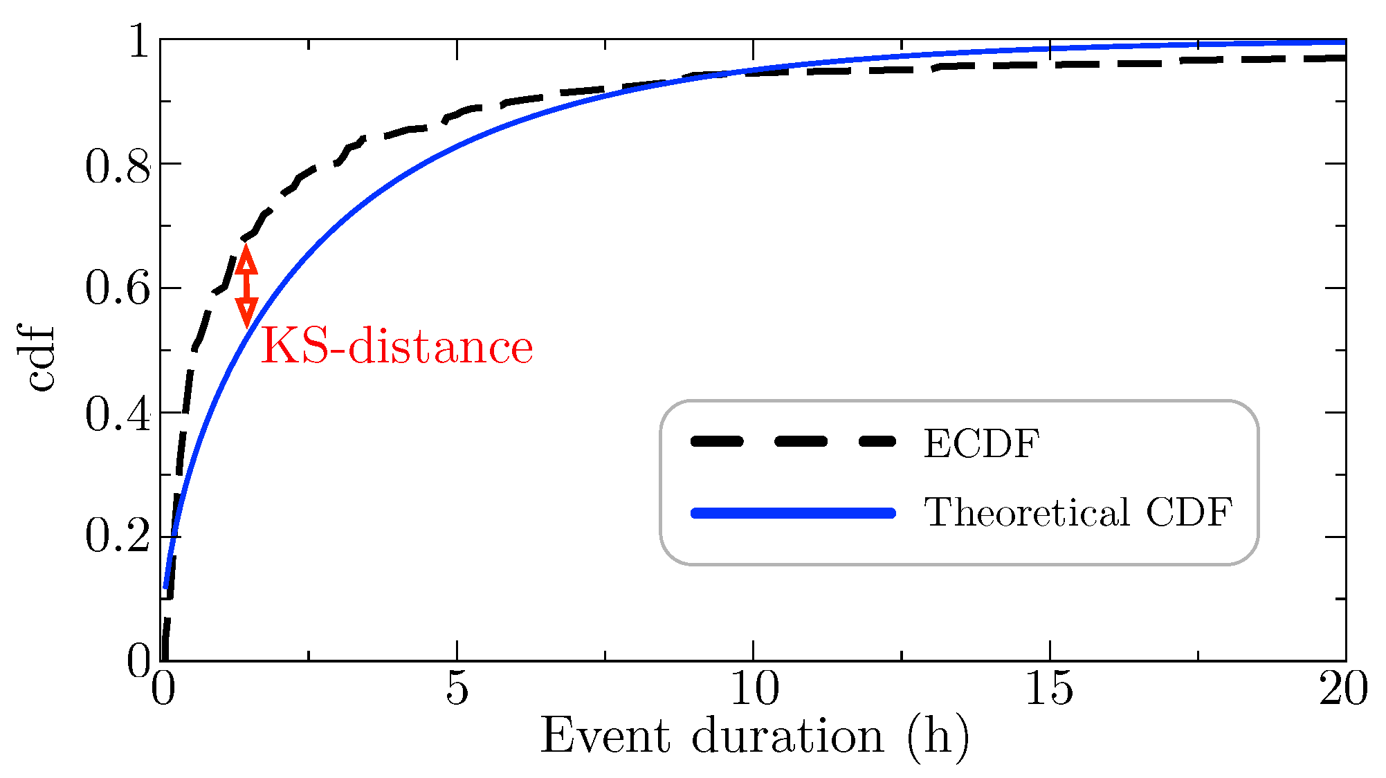
The statistical characterization of low visibility events associated with fog at the A-8 motor-road is discussed in this experimental subsection. The KS-distances (3) between the considered CDFs (see Table 2) and the ECDF for each year and season have been calculated taking into account the two approaches described in Section 2.2, i.e., Maximum Likelihood and L-moments methods. A seasonal analysis has been taken into account, in order to discuss whether the statistical characterization of fog events is independent (or not) from the season of the year. First,

Table 4. Low-visibility events statistics at Mondoñedo station for years 2018 and 2019, and for the 2000 m threshold.

	Fog Events Average Duration (Minutes)		# of Fog Events
	2018	2019	2018	2019
Winter	122.69	149.22	285	168
Spring	201.42	144.02	246	246
Summer	317.63	346.98	224	191
Autumn	161.23	81.21	206	276

shows the statistics of the low-visibility events at Mondoñedo in the years of the study (2018 and 2019).

As can be seen, the number of low-visibility events (<2000 m) by season in both years is quite high, over 200 episodes or quite close to 200 in all cases.

In general, the number of fog events does not seem to have a dependence with the season, as in the case of radiative-type fogs, which are associated with cool/cold periods. In this case, since we have here a type of orographic fog, the number of low-visibility events is very similar in all seasons. In fact, as can be seen in Table 4, the longest average duration of the events is found in summer, with durations about 300 min in both years of study. The shortest durations appear in autumn with 81.21 min of average duration in 2019, or winter with 122.69 min in 2018. 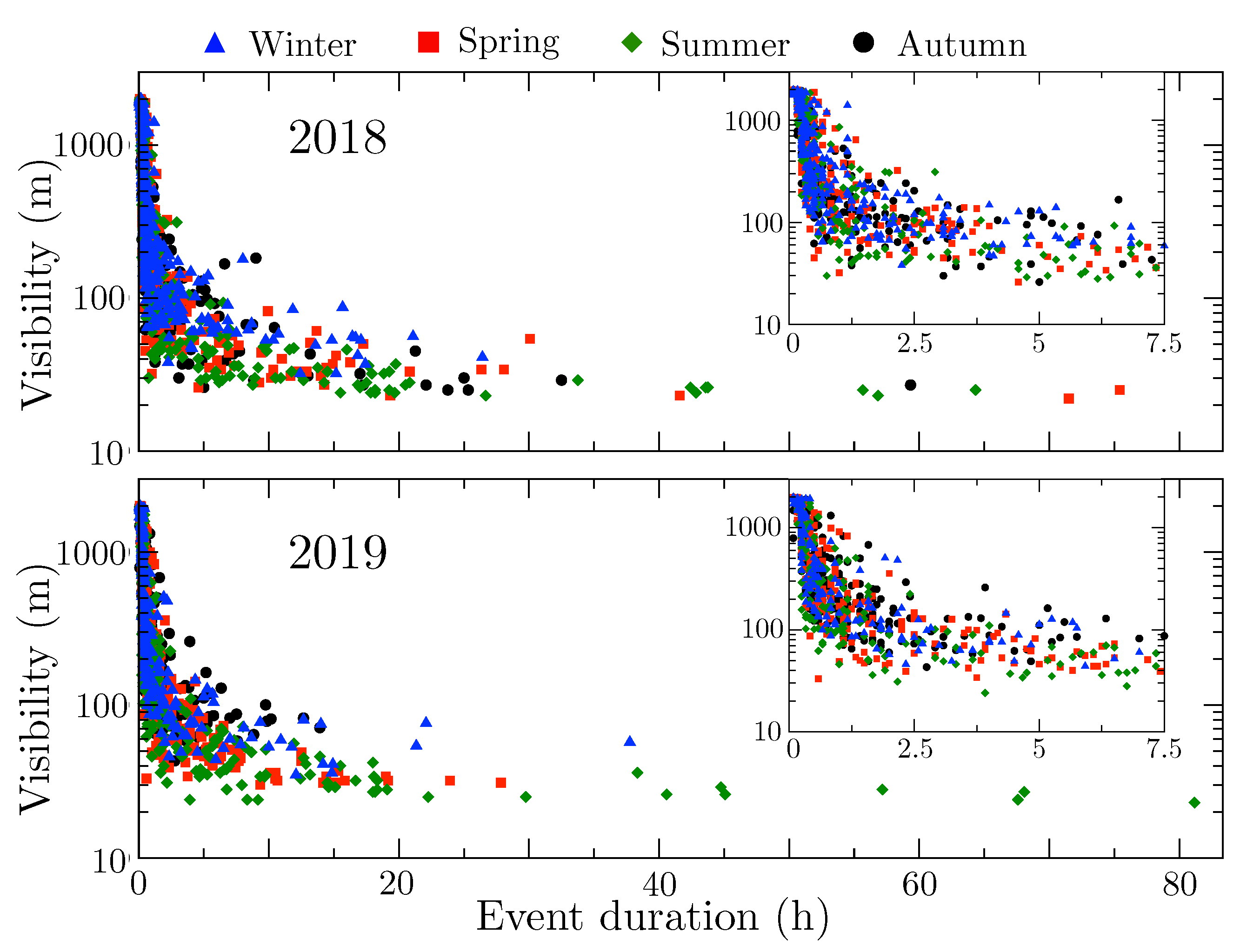Figure 4 shows the different fog events occurred in years 2018 and 2019 at Mondoñedo and their minimal visibility associated value. Observe that those events of longer duration are associated with the lowest visibility minimum value, i.e., denser fog events take longer to dissipate.

We proceed now with the analysis of the probability distributions for fog events duration, by means of minimizing the KS-distance for the two methods of evaluation considered: Maximum Likelihood and L-moments. We start with the Maximum Likelihood case.

Table 5. KS-distances results for the Maximum Likelihood, and for the 2000 m threshold.

	2018				2019
	Winter	Spring	Summer	Autumn	Winter	Spring	Summer	Autumn
EXP	$0.294$	$0.342$	$0.340$	$0.311$	$0.289$	$0.282$	$0.343$	$0.172$
LOG	$0.302$	$0.331$	$0.309$	$0.321$	$0.302$	$0.291$	$0.313$	$0.247$
NRM	$0.301$	$0.347$	$0.302$	$0.337$	$0.305$	$0.286$	$0.317$	$0.262$
GPa	$0.099$	$0.084$	$0.095$	$0.093$	$0.088$	$0.094$	$0.075$	$0.087$
GEV	$0.063$	$0.060$	$0.094$	$0.067$	$0.090$	$0.074$	$0.071$	$0.074$
LN	$0.126$	$0.102$	$0.121$	$0.122$	$0.108$	$0.116$	$0.100$	$0.086$
GAM	$0.189$	$0.186$	$0.169$	$0.176$	$0.175$	$0.177$	$0.178$	$0.154$
EV	$0.403$	$0.463$	$0.402$	$0.460$	$0.427$	$0.393$	$0.417$	$0.384$
LLG	$0.103$	$0.083$	$0.105$	$0.101$	$0.088$	$0.089$	$0.080$	$0.080$
STA	$0.059$	$0.063$	$0.125$	$0.060$	$0.092$	$0.287$	$0.087$	$0.613$

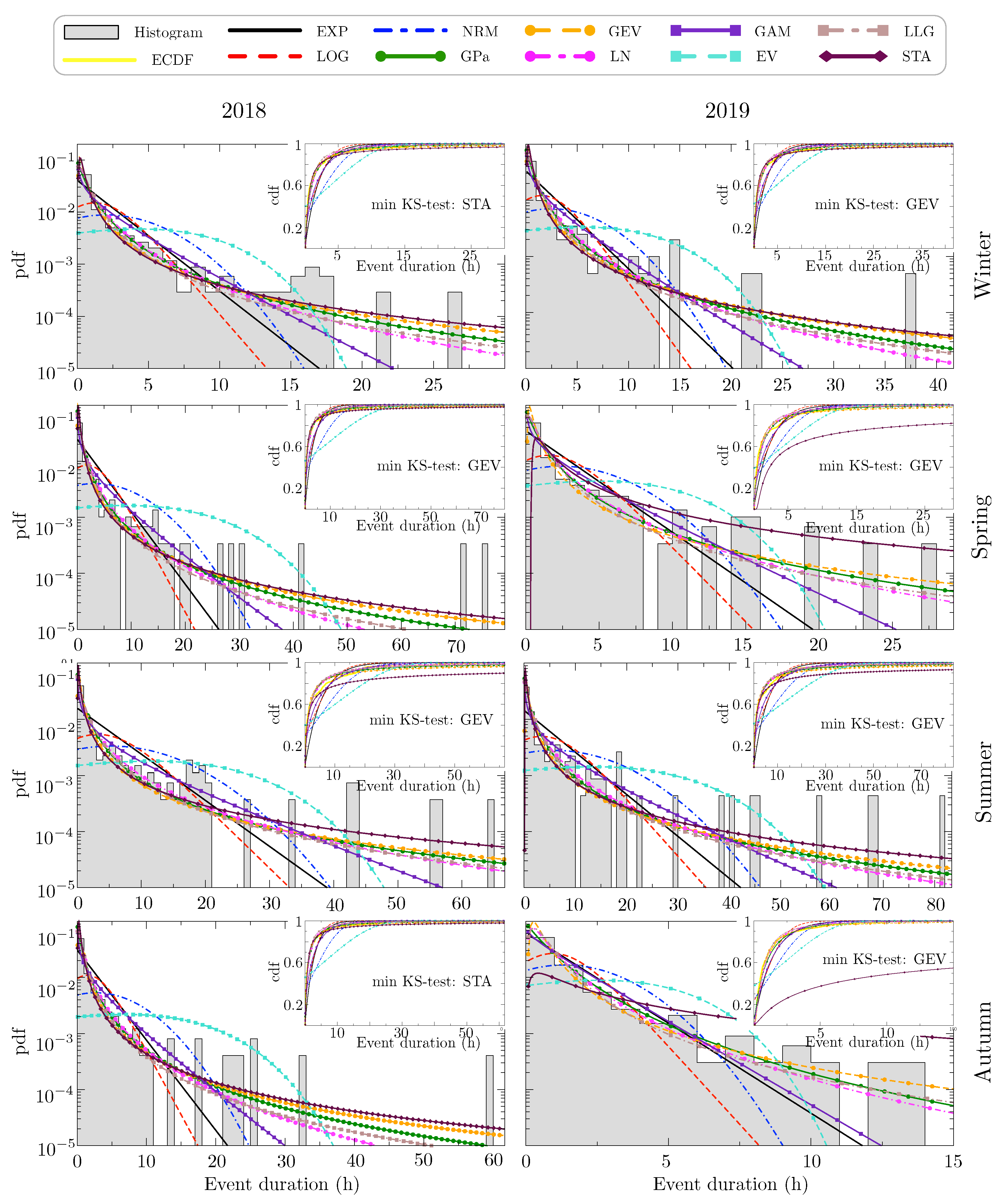
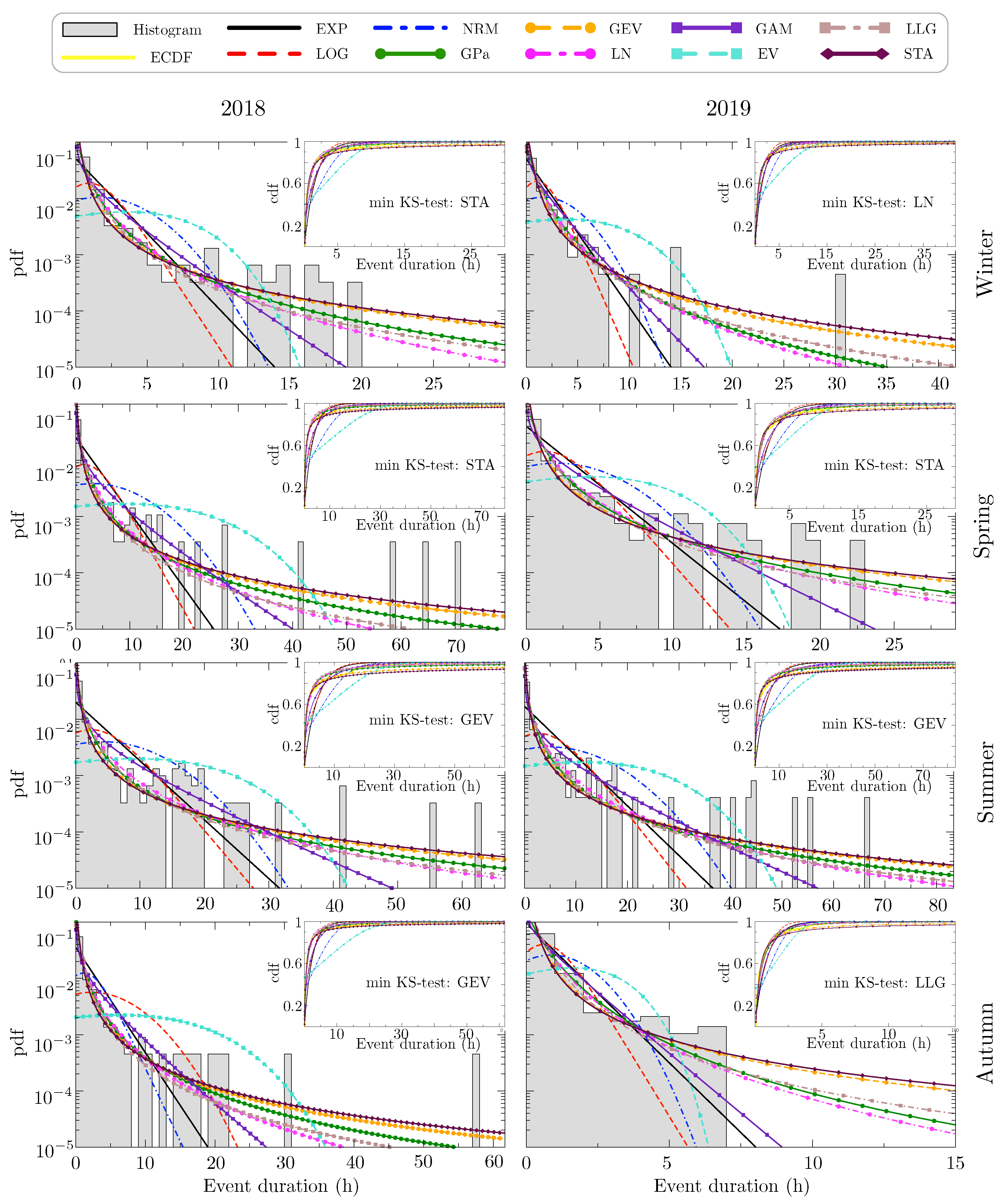
shows the obtained numerical KS-distance using the Maximum Likelihood method. Moreover, Figure 5 illustrates the estimated distributions where the y-axis is plotted logarithmically scaled. In this case, ten distribution functions described in Table 2 were analyzed. We show which distributions best characterize the fog events duration, based on this statistical and seasonal analysis. Specifically we show the KS-distance, which provides a quantitative reference for the best distribution. According to the results, the extremes are significant; i.e., there are many long-term events, or in other words, extreme events of low visibility, and we can see that best results in terms of KS-distance are obtained with the heavy-tail distributions. There are three distributions which fit better than the rest the duration of fog events at Mondoñedo along the seasons: These are the GEV, GPa and STA distributions. These three distributions have the shortest KS-distance and a stationary behavior through the time period. The GEV has a KS-distance around 0.07 through the seasons in both years of study, around 0.09 for the GPa, and 0.06 for the STA in 2018, but with worse values in 2019. LLG also fits well to the data distribution among all seasons around $0.1$ in 2018 and $0.08$ in 2019, even better than STA this last year. This can also be seen more visually in Figure 5, where heavy-tailed distributions such as GEV (in orange) or STA (in burgundy) best fit the data. The same is not true for light-tailed distributions such as EXP (in black) or NRM (in blue) and also for Logistic (LOG) (the red curve). In fact the EXP and LOG, are straight lines far from the origin in logarithmic representation, so that they do not fit very well, or NRM and EV (in cyan) which have a concave shape in this representation. Especially when we find more extreme events in the data since, as previously mentioned, those distributions are characterized by a rapid decrease in the probability of generating extreme values.

If we look at Table 5, we see that, in most seasons, in both years of study, the shortest KS-distance on average through seasons is obtained by the GEV distribution. It is known that this distribution is well suited for estimating the maximum of samples of size n, from sufficiently long sequences of independent and identically distributed random variables [50]. On the other hand, stable type distributions explain more adequately the extreme or rare phenomena, since they usually explain observations with extreme values and skewness. This denotes the presence of heavy tails [51]. This justifies the inclusion of this type of distribution in the study. Note that these distributions are a more efficient alternative to analyze high volatility phenomena due to their capacity to generate extreme values [51]. Finally, the GPa distribution also plays an important role in the EVT, and it is very common in the study of extreme events related to hydrological issues [52,53]. Its adjustment in our results shows a quite stationary behavior (in both methods) in spite of not showing the smallest KS-distance. This is not the case with the short tail distributions used in the study, i.e., EXP, LOG, NRM and EV. These distributions adapt worse to the fog events data than heavy-tail distributions, as they are characterized by a rapid decrease in the probability of generating extreme values, with KS-distance values around 0.3, or even 0.4 for the EV.

Table 6. KS-test results for the L-moment estimation, and for the 2000 m threshold.

	2018				2019
	Winter	Spring	Summer	Autumn	Winter	Spring	Summer	Autumn
EXP	$0.294$	$0.342$	$0.340$	$0.310$	$0.289$	$0.282$	$0.343$	$0.172$
LOG	$0.318$	$0.355$	$0.327$	$0.336$	$0.313$	$0.320$	$0.325$	$0.272$
NRM	$0.302$	$0.340$	$0.313$	$0.325$	$0.297$	$0.307$	$0.308$	$0.260$
GPa	$0.116$	$0.121$	$0.169$	$0.107$	$0.115$	$0.119$	$0.148$	$0.064$
GEV	$0.148$	$0.130$	$0.161$	$0.137$	$0.141$	$0.152$	$0.160$	$0.091$
LN	$0.097$	$0.065$	$0.380$	$0.075$	$0.130$	$0.171$	$0.248$	$0.059$
GAM	$0.144$	$0.240$	$0.080$	$0.223$	$0.107$	$0.110$	$0.215$	$0.091$
EV	$0.496$	$0.517$	$0.506$	$0.510$	$0.498$	$0.488$	$0.509$	$0.449$
LLG	$0.151$	$0.131$	$0.165$	$0.139$	$0.145$	$0.156$	$0.163$	$0.097$

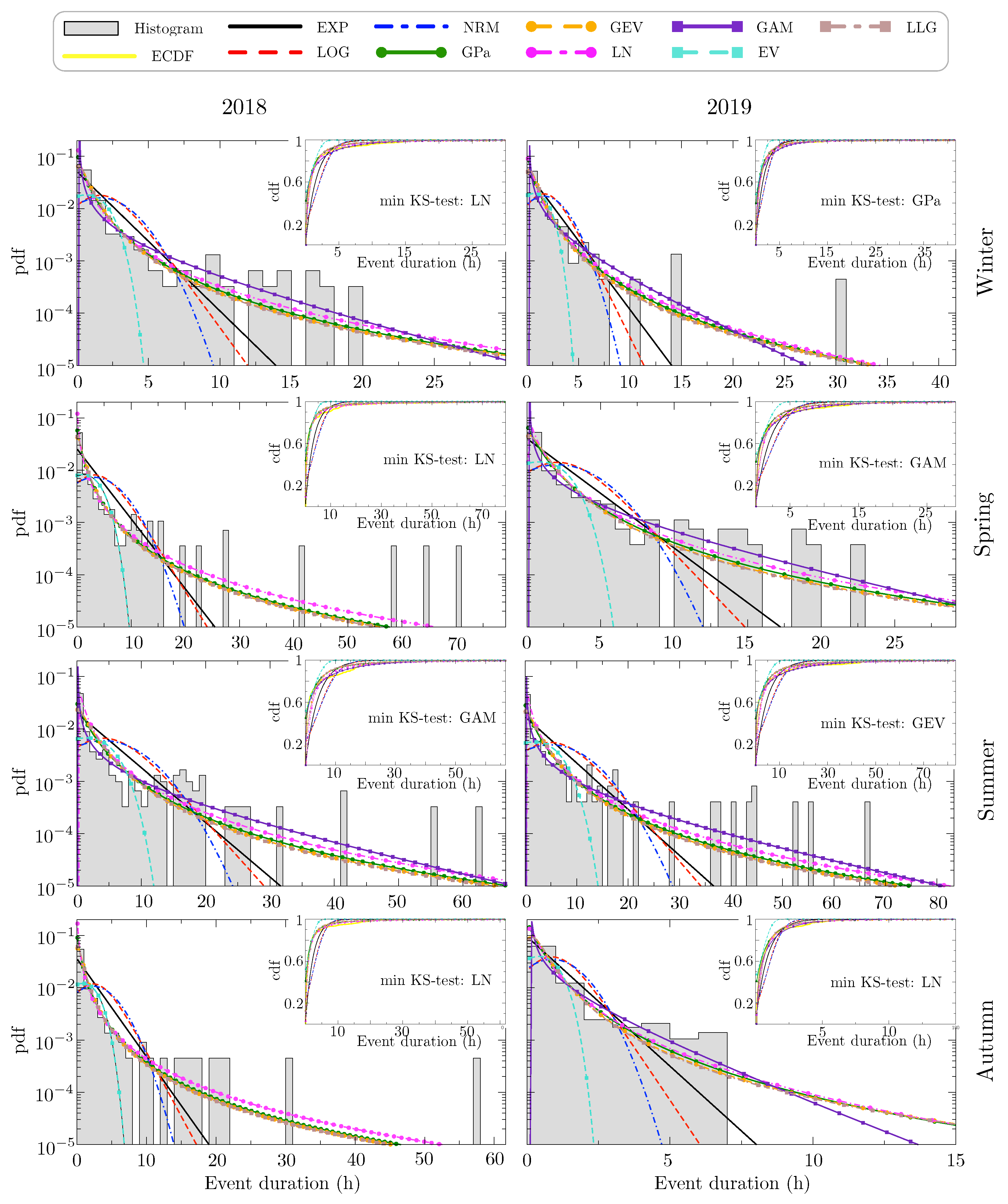
shows the obtained numerical KS-distance using the L-moments method. Furthermore, Figure 6 illustrates the estimated distributions where the y-axis is plotted logarithmically scaled. A total of nine distributions were taken into account in this case, because the moments of the STA distribution do not converge for certain parameters of the distribution. The results show that the distributions that best fit to the fog events in these two years of study are the LN, GAM and GPa with KS-distances around between 0.1 and 0.2. In addition the Log-Logistic (LLG) presents KS-distance stationary values over time, about 0.1. These four distributions are used for modelling hydrological processes or more generally in natural systems [53]. Specifically, the GAM distribution applies to a wide range of physical processes and is related to other distributions: EXP, Pascal, Erlang, Poisson, and chisquare. It is commonly used in meteorological processes i.e., to represent pollutant concentrations and precipitation quantities [54]. Moreover, it is used to measure the time between the occurrence of events when the event process is not completely random [55]. Similarly, in our case, fog events in northwest of Iberian Peninsula, especially in summer, are impulsed by the displacement of the Azores anticyclone. GAM distribution seems to benefit from the L-moments estimation method obtaining lower KS-distances than in case of being estimating by the maximum likelihood method, see Table 5 and Table 6. However, from a qualitatively point of view, GAM probability density function resembles more of a straight line as we move away towards $+\infty$ in Figure 5 and Figure 6. This is not the observed behavior of the data distribution. It is expected that, as soon as the number of samples increases, GAM will fit worse to the data distribution. Once again, heavy-tailed distributions are the ones that best fit to these meteorological situations in Mondoñedo, except for GAM which is a light-tailed and also obtains good results. The light-tailed distributions such as EXP, NRM and EV obtain the poorest fitting to the data. See for example Spring 2018 with a KS-distance of 0.517 in EV distribution, and how together with the LOG, EXP and the NRM they do not adjust correctly to the extreme values of two events of more than 70 h located in the tail of the data distribution.

Observing the obtained results in Table 5, there exist some distributions whose KS-distances hardly vary among seasons, such as, GPa or GEV. This is due to the fact that these distributions explain the low visibility event durations equally well among seasons, even though their durations may change between seasons. On the contrary, those distributions whose KS-distances vary among seasons, such as GAM, cannot adapt to the new conditions by simply changing their parameters.

It is possible to notice some differences between the Maximum Likelihood and L-moments methods in the results previously shown. Note that we obtain slightly better KS-distances in the fittest distributions estimated with the Maximum Likelihood method than with L-moments method. This is the case of GEV, which obtains the best KS results through Maximum Likelihood, below $0.08$, see Table 5. However, LN, which best fits the data distribution, obtains KS-distances around $0.1$ with a high variance among seasons and years, as can be seen in Table 6. It may seem in some instances that the fitting of the GAM distribution is marginally better than that of the LN in some cases. However, it should be noted that, true to its light-tailed nature, the GAM distribution crosses over all of the heavy-tailed distributions (and specifically that of the LN) at large values of fog duration. Therefore, even though GAM may seem a good fit, it fails at large values of fog duration. This is proof that the Maximum Likelihood method fits the main body of the distribution (thus, failing at large values of fog duration) while the L-moment method fits the tails of the present data (failing at low values of fog duration).

As a final note on this point, an accurate statistical characterization of fogs events with extreme-valued distributions can be used to simulate their occurrence at Mondoñedo, within traffic simulators. This way the real effects of deep fog events on traffic causing jams and important circulation problems can be studied.

3.1.1. Discussion: Physical Mechanism

The data used in this study show that, although the number of low visibility events is quite similar in all seasons (see Table 4) they last longer in the warm season. The explanation for this pattern can be found in the high pressure system most influential for the Atlantic and Europe: the Azores Anticyclone. In summer, this pressure system strengthens and reaches its most northerly position [56], bringing northerly winds to the Iberian Peninsula. As have been discussed by some authors [57,58] the main ingredients needed for the formation of the low visibility events that affect the “Alto de O Fiouco” area are northward winds that push warm and humid air masses coming from the sea. Since in this region there is a large mountain barrier of around 600–700 m pretty close to both, the Atlantic Ocean and the Cantabrian Sea, these parcels of air are lifted adiabatically becoming saturated at relatively low levels. In addition, the presence of the typical subsidence inversion caused by the Azores Anticyclone forces the formation of low level layers of clouds (mainly stratus and stratocumulus) which can affect the A-8 motor-road since its elevation at this specific location is quite similar to the level at which these clouds are formed (the so-called lifting condensation level). Furthermore, it should be noted that because this meteorological phenomena is caused by a maritime air mass the number of hygroscopic particles (mainly sea salt) can be considerably higher than normal, which can play a major role in the formation of dense fog events [58].

3.1.2. Statistical Study with Different Thresholds for Defining Low-Visibility Events

The results on statistical characterization of low-visibility fog episodes shown above consider as low-visibility events those under the limit of the visibilimeter (<2000 m, light low-visibility). However, note that this threshold to consider a fog event as low-visibility can be set by the practitioner at alternative values. For example, we can choose different thresholds related to traffic protocols, such as 600 m (moderate low-visibility), 300 m (severe low-visibility), and 50 m (extremely severe low-visibility), all of them with an important effect in secure driving conditions. In fact, visibility below 50 m (extremely severe) very probably leads to motor-road closure.

Table 7. Low-visibility events statistics at Mondoñedo station for the years 2018 and 2019, and for the 600 m threshold.

	Fog Events Average Duration (Minutes)		# of Fog Events
	2018	2019	2018	2019
Winter	102.17	116.72	278	180
Spring	187.32	135.11	237	224
Summer	274.77	283.10	240	220
Autumn	126.67	61.99	226	260

and

Table 8. Low-visibility events statistics at Mondoñedo station for the years 2018 and 2019, for the 300 m threshold.

	Fog Events Average Duration (Minutes)		# of Fog Events
	2018	2019	2018	2019
Winter	97.41	98.90	256	186
Spring	194.56	124.62	235	222
Summer	249.76	293.95	254	204
Autumn	138.47	52.63	185	239

show the statistics for the low-visibility events at A8 motor-road in the years of the study (2018 and 2019), considering low-visibility those events under 600 m and 300 m, respectively. As can be seen, the number of low-visibility events with the new thresholds is similar, between them and also to the case of the threshold set at 2000 m (light low-visibility events). The low visibility event durations are also quite similar for these three thresholds and their proportions among the seasons remain constant. The low visibility events in the warmer seasons continue to be the longest lasting, see Table 4 and Table 7, Table 8 and

Table 9. Low-visibility events statistics at Mondoñedo station for the years 2018 and 2019, and for the 50 m threshold.

	Fog Events Average Duration (Minutes)		# of Fog Events
	2018	2019	2018	2019
Winter	55.43	63.12	34	15
Spring	107.90	60.97	186	133
Summer	156.10	151.48	263	228
Autumn	119.39	16.25	97	3

. This is due to the fact that fog events are usually very intense at Mondoñedo in this season. Table 9 shows the case of the threshold at 50 m. In this extreme severe case, the number of events is very reduced with respect to other thresholds. This indicates that extreme severe low-visibility events are less frequent than moderate and severe events, mainly in winter and autumn, but with a significant incidence in spring and summer.

We repeat here the analysis of the probability distributions for fog events duration, considering low-visibility events defined by setting the thresholds to 600, 300 and 50 m. We consider ten distributions including light and heavy tail distributions, using both the Maximum Likelihood and L-moments methods. In the case of Maximum Likelihood estimation,

Table 10. KS-distances results for the Maximum likelihood, for the 600 m threshold.

	2018				2019
	Winter	Spring	Summer	Autumn	Winter	Spring	Summer	Autumn
EXP	$0.279$	$0.383$	$0.381$	$0.334$	$0.251$	$0.262$	$0.388$	$0.195$
LOG	$0.313$	$0.345$	$0.327$	$0.338$	$0.293$	$0.298$	$0.333$	$0.269$
NRM	$0.310$	$0.355$	$0.318$	$0.355$	$0.313$	$0.295$	$0.326$	$0.271$
GPa	$0.117$	$0.113$	$0.088$	$0.120$	$0.097$	$0.089$	$0.088$	$0.123$
GEV	$0.073$	$0.072$	$0.057$	$0.091$	$0.105$	$0.073$	$0.081$	$0.083$
LN	$0.101$	$0.111$	$0.110$	$0.088$	$0.111$	$0.074$	$0.097$	$0.106$
GAM	$0.171$	$0.202$	$0.187$	$0.190$	$0.137$	$0.147$	$0.193$	$0.153$
EV	$0.401$	$0.465$	$0.415$	$0.476$	$0.448$	$0.400$	$0.417$	$0.374$
LLG	$0.088$	$0.093$	$0.085$	$0.089$	$0.106$	$0.071$	$0.083$	$0.093$
STA	$0.071$	$0.068$	$0.436$	$0.086$	$0.106$	$0.072$	$0.495$	$0.087$

,

Table 11. KS-distances results for the Maximum likelihood, for the 300 m threshold.

	2018				2019
	Winter	Spring	Summer	Autumn	Winter	Spring	Summer	Autumn
EXP	$0.279$	$0.395$	$0.386$	$0.333$	$0.205$	$0.287$	$0.379$	$0.198$
LOG	$0.317$	$0.351$	$0.327$	$0.339$	$0.276$	$0.307$	$0.329$	$0.267$
NRM	$0.313$	$0.357$	$0.312$	$0.352$	$0.310$	$0.297$	$0.320$	$0.267$
GPa	$0.125$	$0.118$	$0.103$	$0.110$	$0.092$	$0.107$	$0.090$	$0.138$
GEV	$0.089$	$0.080$	$0.081$	$0.067$	$0.073$	$0.076$	$0.066$	$0.105$
LN	$0.115$	$0.124$	$0.118$	$0.107$	$0.070$	$0.098$	$0.100$	$0.104$
GAM	$0.158$	$0.200$	$0.186$	$0.196$	$0.139$	$0.166$	$0.175$	$0.159$
EV	$0.403$	$0.457$	$0.422$	$0.469$	$0.450$	$0.389$	$0.411$	$0.366$
LLG	$0.104$	$0.100$	$0.100$	$0.092$	$0.072$	$0.087$	$0.088$	$0.096$
STA	$0.083$	$0.078$	$0.311$	$0.070$	$0.078$	$0.072$	$0.181$	$0.101$

and

Table 12. KS-distances results for the Maximum likelihood approach, for the 50 m threshold. Estimations of autumn 2019 are not possible since there are only three low-visibility events with a threshold under 50 m in that period.

	2018				2019
	Winter	Spring	Summer	Autumn	Winter	Spring	Summer	Autumn
EXP	$0.232$	$0.322$	$0.347$	$0.305$	$0.355$	$0.243$	$0.332$	$--$
LOG	$0.258$	$0.329$	$0.326$	$0.308$	$0.305$	$0.282$	$0.318$	$--$
NRM	$0.299$	$0.342$	$0.317$	$0.303$	$0.358$	$0.262$	$0.301$	$--$
GPa	$0.129$	0135	$0.117$	$0.102$	$0.243$	$0.144$	$0.117$	$--$
GEV	$0.131$	$0.124$	$0.095$	$0.067$	$0.192$	$0.132$	$0.110$	$--$
LN	$0.145$	$0.108$	$0.117$	$0.105$	$0.256$	$0.123$	$0.117$	$--$
GAM	$0.193$	$0.177$	$0.177$	$0.190$	$0.316$	$0.176$	$0.172$	$--$
EV	$0.409$	$0.462$	$0.420$	$0.390$	$0.356$	$0.342$	$0.388$	$--$
LLG	$0.138$	$0.106$	$0.102$	$0.088$	$0.227$	$0.111$	$0.106$	$--$
STA	$0.131$	$0.118$	$0.090$	$0.063$	$0.181$	$0.125$	$0.101$	$--$

show the obtained KS-distance for each distribution, divided by seasons and years. We clearly distinguish two different statistic behaviors in the results obtained. Low-visibility events defined by thresholds under 600 and 300 m have a very similar behavior than that defined by a threshold at 2000 m, as can be seen in Table 10 and Table 11, respectively. Figure 7 shows the distributions estimated by the Maximum Likelihood method for all seasons in 2018 and 2019 at the 300 m threshold which helps us along the discussion. GEV, GPa and STA are still the distributions which best fit the data, with KS-distances below $0.1$ for both the 600 and 300 m thresholds. Their good approximation to the data distribution is clearly presented in Figure 7 for the 300 m threshold. The non-negligible probability of the extreme events is responsible of the good results reported by these heavy-tail distribution, similar to those obtained with a 2000 m threshold, see Table 5 and Figure 5. GEV obtains the best KS-distances in most of seasons of the two years analyzed, closely followed by STA. Both distributions report KS-distances around $0.08$ in most seasons. Even for autumn 2019 at the 300 m threshold which is a season with no extreme fog events, see Table 11 and Figure 7. However, STA fails to fit data distribution in both summers, where most of the extremes take place. LLG and GPa obtain larger KS-distances than the previous one between $0.09$ and $0.11$, but still with good results. The results of the rest of the evaluated distributions are far from these ones discussed previously, especially that provided by the light-tail distributions EXP, LOG, NRM and EV, which are characterized by a quick decrease in probability. In Figure 7, we see that EXP and LOG distributions are straight lines with different slopes, mainly far from the origin, and EV and NRM have concave shape, which does not fit the data distribution trend. The KS-distances obtained by these distributions are above $0.3$ for both thresholds. In the case of low-visibility events defined by the threshold of 50 m, the behavior changes slightly with respect to the case of the threshold situated at 2000 m, see Table 12. Again, the best KS-distances are obtained by the heavy-tail distributions GEV, and STA, but their KS distances are now around $0.1$ with more variations among the seasons. The light-tail distributions still obtain the worst KS-distances, but they decrease respect to the previous threshold. We cannot estimate distributions of autumn 2019 for a threshold of 50 m since the number of low-visibility events in this season is only 3.

Table 13. KS-test results for the L-moment estimation, for the 600 m threshold.

	2018				2019
	Winter	Spring	Summer	Autumn	Winter	Spring	Summer	Autumn
EXP	$0.279$	$0.383$	$0.381$	$0.334$	$0.251$	$0.262$	$0.388$	$0.195$
LOG	$0.329$	$0.372$	$0.349$	$0.356$	$0.299$	$0.309$	$0.353$	$0.288$
NRM	$0.319$	$0.358$	$0.334$	$0.343$	$0.291$	$0.298$	$0.336$	$0.273$
GPa	$0.124$	$0.166$	$0.184$	$0.129$	$0.122$	$0.128$	$0.182$	$0.087$
GEV	$0.129$	$0.163$	$0.184$	$0.137$	$0.125$	$0.129$	$0.174$	$0.122$
LN	$0.094$	$0.099$	$0.316$	$0.069$	$0.161$	$0.162$	$0.279$	$0.082$
GAM	$0.241$	$--$	$0.179$	$--$	$0.261$	$0.192$	$0.214$	$0.092$
GEV	$0.504$	$0.529$	$0.518$	$0.522$	$0.495$	$0.495$	$0.523$	$0.471$
LLG	$0.132$	$0.164$	$0.186$	$0.138$	$0.129$	$0.133$	$0.176$	$0.127$

,

Table 14. KS-test results for the L-moment estimation, for the 300 m threshold.

	2018				2019
	Winter	Spring	Summer	Autumn	Winter	Spring	Summer	Autumn
EXP	$0.279$	$0.395$	$0.386$	$0.333$	$0.205$	$0.287$	$0.379$	$0.198$
LOG	$0.334$	$0.372$	$0.351$	$0.350$	$0.290$	$0.326$	$0.333$	$0.265$
NRM	$0.323$	$0.360$	$0.337$	$0.341$	$0.277$	$0.315$	$0.318$	$0.253$
GPa	$0.133$	$0.174$	$0.197$	$0.110$	$0.077$	$0.148$	$0.189$	$0.106$
GEV	$0.135$	$0.170$	$0.193$	$0.125$	$0.098$	$0.144$	$0.176$	$0.123$
LN	$0.104$	$0.108$	$0.411$	$0.052$	$0.057$	$0.193$	$0.341$	$0.093$
GAM	$0.121$	$--$	$0.106$	$--$	$0.199$	$0.104$	$0.211$	$0.146$
EV	$0.507$	$0.533$	$0.518$	$0.522$	$0.481$	$0.502$	$0.521$	$0.472$
LLG	$0.138$	$0.171$	$0.195$	$0.125$	$0.102$	$0.147$	$0.178$	$0.130$

and

Table 15. KS-test results for the L-moment estimation, for the 50 m threshold.

	2018				2019
	Winter	Spring	Summer	Autumn	Winter	Spring	Summer	Autumn
EXP	$0.232$	$0.322$	$0.347$	$0.305$	$0.355$	$0.243$	$0.332$	$--$
LOG	$0.267$	$0.359$	$0.337$	$0.327$	$0.398$	$0.299$	$0.328$	$--$
NRM	$0.250$	$0.349$	$0.322$	$0.313$	$0.381$	$0.285$	$0.316$	$--$
GPa	$0.113$	$0.153$	$0.177$	$0.120$	$0.242$	$0.156$	$0.183$	$--$
GEV	$0.144$	$0.151$	$0.166$	$0.134$	$0.274$	$0.146$	$0.169$	$--$
LN	$0.114$	$0.121$	$0.238$	$0.094$	$0.334$	$0.261$	$0.320$	$--$
GAM	$0.088$	$0.161$	$0.125$	$0.175$	$0.176$	$0.173$	$0.140$	$--$
EV	$0.477$	$0.520$	$0.516$	$0.502$	$0.472$	$0.484$	$0.511$	$--$
LLG	$0.160$	$0.153$	$0.169$	$0.142$	$0.304$	$0.154$	$0.172$	$--$

present the KS-distances obtained in cases when the L-moments method is used for estimating the distributions, with thresholds at 600, 300 and 50 m, respectively. Figure 8 shows the distributions estimated by the L-moments method for all seasons in both 2018 and 2019 at the 300 m threshold. The distributions that best fits to the fog events for the 600 and 300 m thresholds is still the LN, and GPa but with higher values respect to the 2000 m threshold, around $0.1$, and $0.13$, respectively, see Table 13 and Table 14. GAM obtains good KS-distances at the 300 m threshold but not in 600 m and varies along the seasons. Furthermore, GAM struggles to fit data in spring and autumn 2018 due to the used L-moments implementation code. The reason is that the duration of low-visibility events in summer is higher than in other seasons, and GAM did fit such wide range of durations with a good accuracy, since they are straight lines far from the origin in the y-log-scaled Figure 8. GEV also fits were to the data distribution even better than fixing a 2000 m threshold, around $0.13$. The light-tail distributions do not fit the data; although, they obtain better KS-distance than in the case of the 2000 m threshold. EXP, LOG, NRM or EV do not fit the data distribution well as their tail decreases quickly, see Figure 8. Focusing on the results obtained by fixing a threshold at 50 m, Table 12 shows similar results to the previous thresholds for the L-moment estimation. Again, the distributions with best KS-distances are GAM, LN and GPA, with values above $0.11$, higher than in previous thresholds. However, the KS-distances obtained by EXP, EV, NRM are lower than the obtained by fixing 600 and 300 m thresholds. Note that distribution estimations for autumn 2019 do not appear in Table 12, since only three extreme low-visibility events occurred, not enough for the parameter estimation.

3.2. Prediction of Fog Events at A-8 with ELMs

The results obtained with an ELM in the short-term prediction of low-visibility events due to fog at the A-8 motor-road are presented in this section. For ensuring the independence of the partition data in training and test sets, as well as the performance of the regressors, a K-fold cross-validation procedure was carried out [10,59]. The folding was set to $K=10$, and each set consists of an $80\%$ to train and $20\%$ to test. Using the full dataset spanning from 1 January 2018 to 30 November 2019, data are randomly selected, breaking the sequence in the data, in order to bring heterogeneity to the values of the samples.

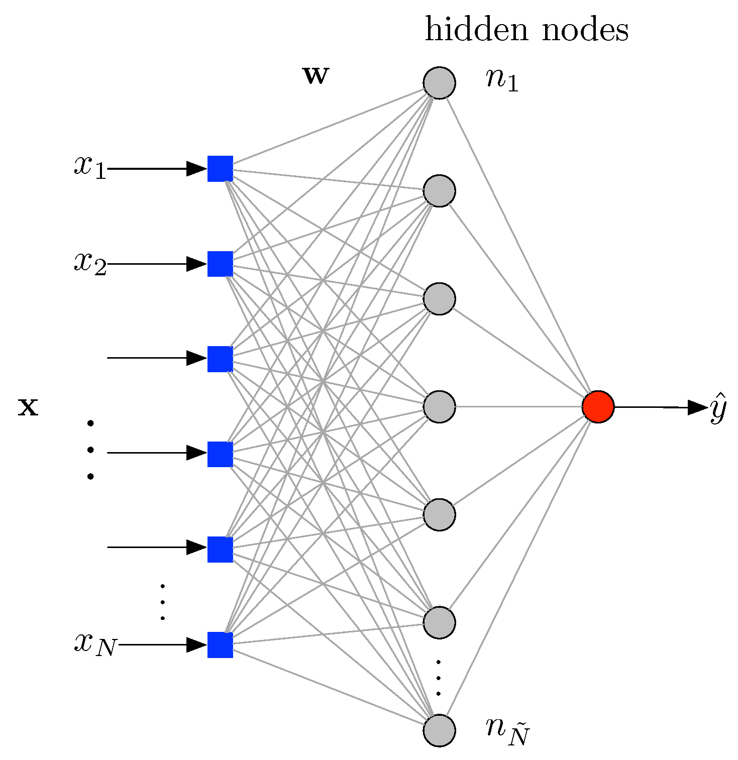
The ELM model considered in this paper has the following characteristics: neurons in the hidden layer are designed with sigmoid activation function. The optimal number of neurons is chosen from a large pool (50–150, in an increment of 1), which passes through the hidden layer, one by one, during the validation phase. In addition to the atmospheric features considered, we will also use the 4 time instants prior to the target we want to predict (t), as predictors, i.e., we will use the target values at $t-1$, $t-2$, $t-3$ and $t-4$. We should note that in all experiments the input–output data pair, ${\left\{({\mathbf{x}}_i,y_i)\right\}}_{i=1}^n$, for both ELMs has a time resolution of half an hour (where n stands for the total number of half-hour intervals in the database); hence, the forecasting time-horizon was set to 30 min ahead estimation (instant t) of the visibility. Finally, the experiments will consist of launching 10 executions of each algorithm for each proposed scenario, and average the results of them.

In order to better analyze the ELM performance, a wrapper feature selection process was carried out. This procedure consists of launching as many ELMs as combinations of characteristics we have in a reduced validation set, to find the set of predictors that provides the least error at the output (best set of features). Note that we have 10 features (only the atmospheric features are considered in this process) for this problem (see Table 1), which means that we have to launch a total of 1024 ($2^{10}$) ELM models (prediction problems) to obtain the best set of characteristics (inputs). Note that we need an extremely fast-training algorithm such as ELM to carry out this feature selection analysis, since otherwise the computation time required would be extremely high. The results obtained in the feature selection process provided two sets of features as best results: the first one included a total of nine characteristics: Accumulated precipitation, Salinity, Relative humidity, Air temperature, Floor temperature, Dew temperature, Global solar radiation, Wind speed and Atmospheric pressure, with a Root Mean Square error (RMSE) of $378.54$ m in the validation set. A second best set with a total of three characteristics was also obtained: Accumulated precipitation, Relative humidity and Global solar radiation; with a RMSE of $381.36$ m in the validation set. The rest of features combination produced worse results, so we have kept these two best sets for carrying out the experiments. In order to compare the results, we used the Persistence Prediction Operator (PPO${}_1$), a well known operator described by the following equation:

$$x(t+1)=x\left(t\right).$$

(6)

The generalized Persistence prediction operator (PPO${}_M$) uses the M last time steps to infer the prediction and can be also defined as:

$$x(t+1)=\frac{1}{M}{\displaystyle \sum _{i=1}^M}x(t-i).$$

(7)

In our experiments, we fix $M=4$ referenced as (PPO${}_4$).

Prediction Results

Table 16. Prediction error results by the ELM and PPO approaches, and computational running time (Train-t and Test-t) by ELM.

	ELM-9		ELM-3		PPO${}_1$		PPO${}_4$
	Avg	Std	Avg	Std	Avg	Std	Avg	Std
$r^2$	$0.80$	$0.01$	$0.80$	$0.01$	$0.77$	−	$0.72$	−
RMSE (meters)	$394.82$	$9.50$	$393.56$	$5.28$	$418.09$	−	$477.65$	−
Train-t (seconds)	$18.99$	$1.00$	$16.06$	$0.65$	−	−	−	−
Test-t (seconds)	$0.05$	$0.01$	$0.03$	$0.004$	−	−	−	−

shows the average and standard deviation results (10 runs of the algorithms) obtained by the ELM, when we use 9 or 3 characteristics as predictors (ELM-9, ELM-3), and the obtained by the PPO, which uses the last (PPO${}_1$) and the four last time steps (PPO${}_4$) for comparison. These results to evaluate the ELM performance are given in terms of the Pearson’s correlation coefficient, $r^2$, the RMSE and the computation times, both training (Train-t) and test (Test-t). It can be observed that the ELM approach is able to obtain the best results, with an RMSE of 393.56 m and an 80% of $r^2$ when 3 features are used as predictors. If we compare these results with the case of ELM-9, we can observe a slight difference in terms of RMSE, with a value of 394.82 m, but a similar value for $r^2$. Therefore, the ELM model works slightly better with fewer features, achieving good results using less computation time, in particular taking 16.06 and 0.03 s in Train-t and Test-t, respectively in ELM-3, against the 18.99 and 0.05 s for Train-t and Test-t in the ELM-9 case. Based on these results we can see that the selection of features has an effect on the prediction process by using the ELM approach. The results obtained by the PPO are considerably worse. If we analyze the PPO for both variants, PPO${}_1$ and PPO${}_4$, we can see the poor performance in terms of RMSE and the worse one in $r^2$. In this case, the best results are obtained for PPO${}_1$ with an RMSE of $418.09$ m and $0.77$ in $r^2$, below the $0.80$ of the ELM. The difference with respect to the case of PPO${}_4$ is larger than in the ELM at least in terms of RMSE which obtains $477.65$ m. In terms of $r^2$, PPO${}_4$ obtains $0.72$, similar to the PPO${}_1$. We deduce that, in case of PPO, it is better to use the last time step than four time steps for obtaining the prediction. This is because the visibility time series is quite volatile, and using PPO${}_4$ (7) strongly smooths the time series. Note that the computation time required to train the ELM is acceptable. PPO reaches real time as the predicted series is simply the mean given by Equation (7).

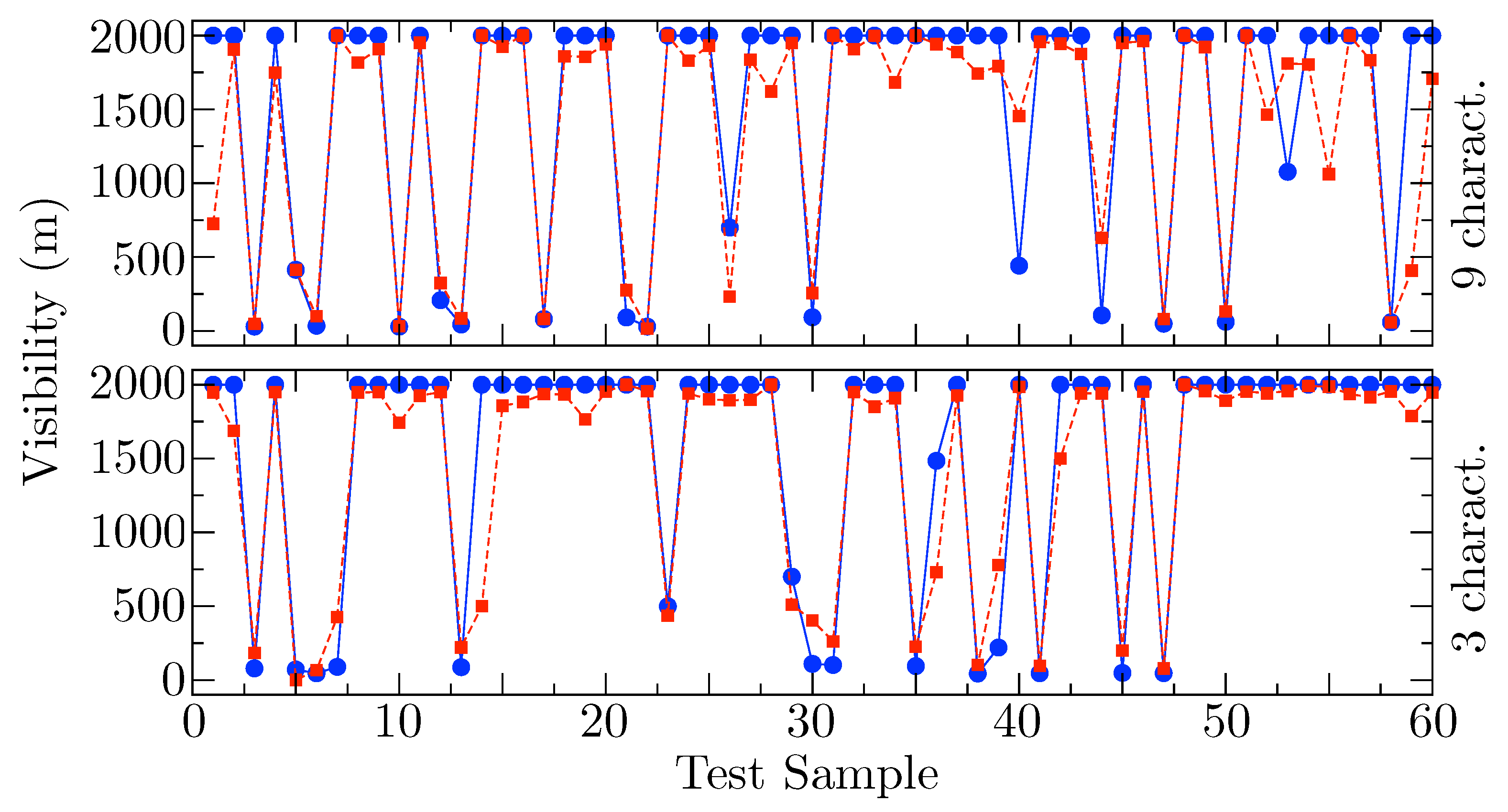
Figure 9 shows a temporal representation of the predicted visibility variable (in red) versus the measured values of this variable (in blue), by the ELM with nine features and three features. It is possible to see that in both cases the performance of the ELM is excellent in this prediction problem, showing good behaviour even in the deepest fog events. Moreover, these good results are obtained regardless of the set of samples we test. As can be seen, in the prediction graphs with nine and three features as predictors, different test samples are used to quantify the performance of the model, which is very interesting to corroborate the good performance of this type of learning machine.

4. Conclusions

In this paper we carried out a detailed study on low-visibility events due to fog at the A-8 motor-road, Galicia, Spain. In this zone there are frequent episodes of low-visibility events due to orographic fog from the Cantabrian sea, which deeply affect the traffic in the road. First, we statistically characterized the fog events’ duration with different distributions, including light and heavy-tail distributions, in a seasonal analysis. Two different approaches were considered to estimate the parameters associated with the distributions, the Maximum Likelihood criterion and the L-moments approach. In both cases we showed that the heavy-tail distributions (extreme distributions) are more suitable to describe the duration of low-visibility events at the A-8 motor-road, independently of the season considered. We can state that three of the heavy-tailed distributions are the best fit in most cases. These are the GEV, the GPa and LN. These three distributions present the smallest KS-distances values in most cases, especially in those where this phenomenon of dense and long-lasting fogs takes place: in summer. LLG also obtains consistently very good results closed to the previous ones among all seasons of the studied years for both estimation methods. Other distributions such as GAM or STA offer good results in some cases, but this is not the majority. In some cases, GAM reports very good KS-distances when is estimated by the L-moment method, not as good by the maximum likelihood method, even as a light-tailed distribution. We carried out an analysis by considering different visibility thresholds to define the low-visibility events, showing that the results are very similar in light, moderate and severe low-visibility events situations (thresholds of 2000 m, 600 m and 300 m), whereas for extreme severe low-visibility events (less than 50 m), their statistical characterization is different.

Second, we tackled the prediction of the visibility in the zone, by using an ELM regressor. Atmospheric variables collected in-situ such as air and floor temperature, wind speed and direction, pressure, etc. were used as inputs to carry out the prediction. We showed an accurate performance of the ELM with average errors under 400 m in all cases, improving by far the performance of the persistence prediction operator in the problem. In all the experiments carried out, the variance of the prediction results as very low, which indicates that the prediction is accurate, i.e., the ELM obtains a good prediction, even for different low-visibility ranges (light, moderate, severe and extreme severe low-visibility events).

The methods and algorithms presented in this paper have a direct application in dealing with the issues caused by low-visibility events from orographic fog on the A-8 motor-road. The statistical description of the events allows an accurate modeling of low-visibility event’s duration in traffic models simulations. This can be complimented with and accurate prediction of low-visibility events, in order to implement actions to minimize their impact in the traffic of the zone.

Note that some limitations are found in this work, mainly in the capacity of the proposed methods to characterize and predict extreme low-visibility events. Future analysis of low-visibility events in the zone can include numerical weather prediction approaches combined with ML algorithms, to help deal with these cases. Numerical methods such as meso-scale models can improve the accuracy of the prediction models, by including new information as input variables. In turn, we can complete real data with numerical weather models simulations, in order to produce larger datasets to improve the accuracy of the statistical models for low-visibility events’ description.