Article

Basic Statistical Estimation Outperforms Machine Learning in Monthly Prediction of Seasonal Climatic Parameters

1
Department of Computer Science, University of the Western Cape, Cape Town 7535, South Africa
2
Department of Science and Mathematics, Texas A&M University-Central Texas, Killeen, TX 76549, USA
3
Department of Physics and Astronomy, University of the Western Cape, Cape Town 7535, South Africa
*
Author to whom correspondence should be addressed.
Atmosphere 2021, 12(5), 539; https://doi.org/10.3390/atmos12050539
Submission received: 25 March 2021 / Revised: 7 April 2021 / Accepted: 14 April 2021 / Published: 23 April 2021
(This article belongs to the Special Issue Statistical Methods in Weather Forecasting)

Abstract

:
Machine learning (ML) has been utilized to predict climatic parameters, and many successes have been reported in the literature. In this paper, we scrutinize the effectiveness of five widely used ML algorithms in the monthly prediction of seasonal climatic parameters using monthly image data. Specifically, we quantify the predictive performance of these algorithms applied to five climatic parameters using various combinations of features. We compare the predictive accuracy of the resulting trained ML models to that of basic statistical estimators that are computed directly from the training data. Our results show that ML never significantly outperforms the statistical baseline, and underperforms for most feature sets. Unlike previous similar studies, we provide error bars for the relative performance of different predictors based on jackknife estimates applied to differences in predictive error magnitudes. We also show that the practice of shuffling data sequences which was employed in some previous references leads to data leakage, resulting in over-estimated performance. Ultimately, the paper demonstrates the importance of using well-grounded statistical techniques when producing and analyzing the results of ML predictive models.

1. Introduction

Recent advances in computing have shifted the focus of scientific communities from a data-scarce to a data-rich research environment [1]. This paradigm shift, known as the fourth paradigm of science, and often referred to as the era of “big data” [2], has emerged from the move of big data and AI into our daily lives and the pervasiveness of these two technologies, which are (i) leading to an explosion in innovation, competition, and productivity [3], (ii) causing a dramatic shift to data-driven research [4], and (iii) unleashing the benefits of data-intensive applications.
Climate science is a research field where data-driven models based on machine learning (ML) have become popular [5]. A major focus of climate science is the understanding and prediction of climate parameters such as rainfall and temperature [6] and many others. For many practical climate-influenced decisions where prediction times of months to a decade are likely to be the most important [7], providing accurate models to predict climatic parameters on these time scales is critical. The remarkable successes of ML and deep learning in a variety of fields such as computer vision and natural language processing suggests that this success may be extended to climate science as well.
However, there is a concern regarding how effective and legitimate these ML models are to address real world applications in climate science. This is reason for enthusiasm, but also for skepticism, as it is all too common to make excessive claims for new techniques, which turn out not to live up to their initial promise, as exemplified by Gartner’s hype cycle model [8]. There are already several examples in the literature that show that ML does not always live up to its hype. A recent overview study reviewed several papers that used recurrent neural networks for top-n recommendation tasks, and found that a simple model using K-nearest neighbors outperformed most of the more sophisticated models [9]. One major deficiency identified by the study was the use of defective or weak baselines when quantifying the performance of newer proposed models. Other papers that also reached the conclusion that sophisticated ML models do not necessarily outperform simpler models include [10,11,12,13].
One key feature of ML methods is that they make no assumptions about the underlying distribution of inputs. This can be both an advantage and a disadvantage. The advantage is that ML methods can be applied to a wide variety of datasets without having detailed knowledge of the statistics of the individual datasets. The disadvantage is that ML may miss important characteristics of particular datasets. For this reason, if the user has some knowledge of the dataset’s distribution, it is important to compare ML predictors with statistical estimates based on the presumed distribution. Such statistical estimates have the advantage that they are simple to calculate, require no training, and are easy to interpret [14].
One deep flaw in most papers in the literature is that accuracy estimates for ML methods are given (such as R 2 or root mean squared error) without providing error bars on these estimates. Hence, it is impossible to tell whether or not differences between methods are statistically significant. This may be one reason why different investigators often reach different conclusions about the relative effectiveness of different ML methods. For example, Armstrong et al. [15] concluded from an analysis in the context of ad hoc retrieval tasks that numerous published papers report mutually contradictory conclusions concerning ML model performance.
Another concern is that some common pre-processing practices produce data leakage, so that ML algorithm accuracies are over-reported. Some examples of such practices are: data shuffling, whereby researchers randomly shuffle the data [11,16,17,18,19,20,21,22,23]; data imputation methods that use statistics (such as averaging) calculated on the entire data set, including both training and testing [24,25,26]; and data transformations such as de-seasonalization that also use statistics calculated on the whole dataset [27,28].
It is necessary to investigate the robustness of ML models in different fields of application. The current study is aimed at investigating the above mentioned deficiencies in the area of climatic seasonal parameters. This paper is organized as follows: Section 3 describes the data used; Section 4 discusses the methodology used for climatic parameter prediction; Section 5 shows the results obtained; Section 6 discusses the results; and Section 7 furnishes the conclusions.

2. Literature Review and Scope of the Research

ML is widely used in climatology to construct predictive models based on sequential data [11]. A variety of types of input data are used, including satellite images or periodic samples from gauges or weather stations.
The studies in the literature can be largely divided into two categories in terms of the predicted output: those that predict one or more entire images which provide a visual representation of a given predicted climate parameter on spatial maps of a specific geographical area under review (“whole-image prediction”); and those that predict only a single output representing a given predicted climate parameter at a fixed location (“single-output prediction”).
For whole-image prediction based on sequential images, convolutional neural networks (CNNs) and convolutional long-short term models (ConvLSTMs) are often used due to their ability to perform feature reduction on spatial information. However these models require very large datasets with tens of thousands of images, due the data-intensive training process. For this reason, CNNs and ConvLSTMs are mainly applied to data sets with short time intervals of no more than a few minutes between data points, which are typically much larger than data sets with longer time intervals [29,30,31,32,33,34,35,36,37,38,39,40]. For single-output prediction, a wider range of ML tools and time frames have been used, from linear methods in [17,21,41,42], to ensemble methods in [43,44,45], to hybrid methods in [28,46,47,48], to deep models in [49,50,51,52,53,54,55,56] covering time scales from minutes to years.
From a practical point of view, usually the most important policy decisions involving climate require monthly predictions [7]. Relatively few studies exist which use image data to make monthly predictions [57,58]. When time scales on the order of months or longer are involved, datasets are typically much smaller than those involving shorter time scales. A broad range of ML methods are applied, from simple methods like multilinear regression (MLR) up to advanced neural networks models [13,16,17,18,20,21,24,25,46,47,49,59,60,61,62]. Because of the small data sets used, researchers often perform feature selection/reduction to avoid overfitting. Most often, the selected features in the literature are combinations of features derived from previous time steps in the data, for example, a parameter at month n may be predicted based one or more parameter values taken from months previous to n [25,26,27,46,63].
Because of the rotation of the earth around the sun, monthly time series data like rainfall exhibit a seasonal behavior on a yearly basis (exhibit a yearly periodicity) [64,65]. This is critical to address because traditional time series models tends to rely on the time series being stationary [64,66]. Hence, the authors in [64] saw it as necessary to remove the periodicity in a monthly time series data. They described three ways of going about this: (a) previous lag differencing, (b) seasonal referencing; and (c) monthly mean subtraction, where (c) was identified as the most suitable method for monthly time series data. However, we found that many papers dealing with monthly prediction of climate parameters did not transform the input data to remove seasonality. Some papers accommodate seasonality by including data from month n 12 to predict parameters at month n [13,17,19,20,24,25,27,28,44,49,51,58,60,62,67]. Month n’s time stamp (defined as n mod 12 ) was used as a feature in [19,49], but is not common in the literature.
In a few papers, the authors subtracted the monthly mean averages computed from the whole data set [25,28], with the inclusion of data from month n 12 . This procedure disrupts the integrity of the data by causing data leakage, whereby information from the testing set is introduced into the training set. Other papers make no attempt to account for seasonality [18,22,23,46,48,61,68,69]. Evidently, there is no consistent procedure for dealing with the seasonality aspect of the data; this is one point that we address in this paper.
In the previous section we emphasized the importance of using simple baselines to provide benchmarks to compare with more complicated methods. According to [66], the simplest baseline for predicting time series is to use the previous lag. For short-term image data, the previous image is used as a naive predictor for the next image [36,37,40,70]. As for monthly data, using previous lags as a baseline is not a common practice. Instead, a variety of baselines are used. Some papers use MLR based on previous lags [13,16,17,25], while the authors in [45] used same-month averages. Some papers do not use simple baselines, but rather compare several variations or architectures of more advanced ML methods such as SVR or MLP [26,27,46,63]. In summary, simple baselines are not consistently used in the literature.
The Objectives of the paper are as follows: (a) perform seasonal grid prediction on multiple climatic parameters; (b) investigate multiple untrained baselines, and in particular using a statistical estimator derived from a simple statistical model of the image pixel distributions; (c) analyze the effectiveness of subtracting the seasonality using the monthly average calculated only on the training data; (d) investigate the common feature sets used in the literature; (e) calculate error bars on the relative prediction accuracies of different methods using jackknife estimation applied to pairwise differences between prediction errors; and (f) demonstrating the effect of data leakage on the reported performance.
Our results show that across all climatic parameters studied, a very limited feature set (time stamp with spatial information) without seasonal subtraction outperforms feature sets that use previous lags, with or without seasonal subtraction. Furthermore, an untrained baseline based on a simple statistical model can out perform more sophisticated ML tools. Furthermore, handling data inappropriately so that data leakage occurs (as has been done in some previous papers) can lead to significant overestimation of predictive performance.

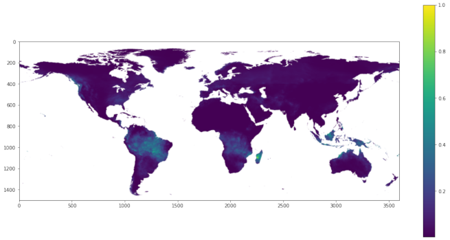
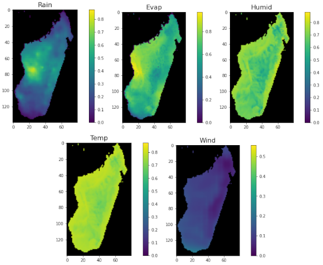
3. Data and Area of Interest

The climatic data were obtained from the NASA GESDISC data archive, which is accessible to users registered with NASA Earthdata [71]. The dataset used is obtained from the Famine Early Warning Systems Network (FEWS NET) Land Data Assimilation System (FLDAS). FLDAS contains monthly image data for 28 fields such as rainfall flux, evaporation, and temperature [72] with a spatial resolution of 0.1 × 0.1 . The data are archived in netCDF format, where it can be manipulated and displayed using freely available software packages within python and R. NASA also supplies a cross-platform application called Panoply that can be used to plot the data [71].
The downloaded data set for each parameter used contains 228 satellite frames on a monthly basis, between January 1982 and December 2000. Images depict the entire globe at a resolution of 1500 × 3600 pixels. Figure 1 shows a sample image of rainfall. In general, the images are color coded to provide information about the relevant parameter. In the current study, the climatic parameters used are rainfall, evaporation, humidity, temperature, and wind speed.
To limit the computational load, we focused our prediction on Madagascar. Madagascar is the world’s fourth largest island with an area of about 592,000 km 2 [73], and is separated from Mozambique on the main African continent by about 400 km [73]. The climate on the island is subtropical and is characterized by a dry season from May to October and rainy season from November to April [74,75]. Table 1 summarizes the characteristics of the Madagascar image data used in our study, which was extracted from the original FLDAS data.
Madagascar is currently facing several challenges due to the potential impact of climate change on the agricultural sector, which can threaten food security [76,77,78,79], especially since farmers in the country are estimated to be 70% of the population [74]. Example images of the five climatic parameters used at a specific arbitrary timestamp are provided in Figure 2. The figure shows normalized values of five climatic parameters, namely rainfall, evaporation, humidity, temperature, and wind.

4. Methodology

Figure 3 shows a flowchart of the system created and used to make predictions in this research. The end goal of the system is to predict monthly rainfall, evaporation, humidity, temperature, and wind speed images on a pixel level, using a sequence of previous images as an input. The rest of this section describes the progression through the flowchart in the figure in detail: first we discuss the pre-processing of the images and the preparation of the data set; then we describe feature selection; and finally, we indicate the tools used. The code together with the results are available on GitHub at https://github.com/EslamHussein55/Climatic-parameters (accessed on 16 April 2021).

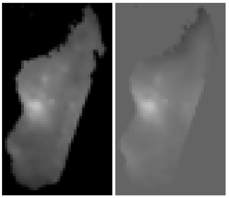
4.1. Image Pre-Processing

All images in the parameter datasets were cropped to a rectangle of size 140 × 80 that includes the Madagascar land area. We transformed the image pixels to greyscale (0–255) and re-sized the images to 70 × 40 to further reduce their complexity. In view of the fact that extreme values are a common occurrence in geophysical parameter data, pixel values were regularized by replacing them with their square roots, following the example of [57,80,81]. Since our study is concerned with relative performance of different algorithms rather than absolute performance, for simplicity we did not remove over-ocean pixels, which are constant in all images and hence perfectly predicted.
We mentioned previously that some authors recommend transforming time series data to remove seasonality, while many authors do not follow this recommendation. To evaluate the effectiveness of transforming time series, we created two input data sets (denoted as `raw’ and `de-seasonalized’) for each of the five parameters. The raw dataset contains the original data, while the de-seasonalized data is transformed by subtracting same-month averages. Care was taken to compute monthly averages based only on the training data to prevent data leakage. For illustrative purposes, Figure 4 shows example raw and de-seasonalized images for rainfall.

4.2. Data Preparation

We prepared the data in a sliding window fashion, similar to the following studies [35,82,83,84,85]. Figure 5 shows how pixels at a given location in a 12 month window are used to predict the corresponding pixel at the same location in the 13th month. In the figure, the symbols {f [ 0 ] , , f [ 11 ] } refer, respectively, to the frames { 12 , , 1 } months prior to the predicted frame, respectively.
As shown in Figure 5, the datasets were used to produce sequences consisting of 12 consecutive months. All datasets were divided into training and testing sets, where the training set was made up of sequences occurring earlier in the dataset, and the testing set made up of sequences that followed those in the training set. This technique of maintaining chronological order when dividing the datasets into training and testing sets helps avoid the problem of information leakage into the trained model from the future [66]. Applying the sliding window generated 216 sequences with the first 156 used for training, and the rest as testing. Although the number of images appears relatively small, the training task is nonetheless computationally expensive since the training process utilizes 156 × 70 × 40 input vectors. This explains why previous similar studies also use relatively few images; for example [86] trains on only 47 images.

4.3. Feature Selection

Feature selection is critical to increasing training efficiency and model accuracy. Based on the reviewed literature for monthly prediction, we tested a variety of feature sets to understand the system mechanism. We also added in features systematically and assessed whether or not added features gave clearly better performances to ensure model parsimony and avoid overfitting [87]. The feature sets are described in the following subsections.
We first created a list of 12 candidate features for image prediction consisting of pixel values at the same location for the 12 prior months. To select a variety of these features, we prepared the data using the sliding window algorithm, where each 12-month window was used to predict the 13th month. Based on previous literature [13,17,18,19,20,22,23,24,25,26,27,28,44,45,46,47,48,49,58,59,61,62,67,68,69,88], we included the following feature sets:
  • f[0]: same-pixel values from frames 12 months previous;
  • f[11]: same-pixel values from the previous month;
  • f[0, 11]: same-pixel values from 12 months previous and the previous month;
  • f[0, 1, 2, 11]: same-pixel values from { 12 , 11 , 10 } months previous and the previous month;
  • f[0, 1, 10, 11]: same-pixel values from { 12 , 11 } months previous and the previous two months.
Given the geographical variation and seasonal nature of the dataset used, the following spatio-temporal features are also used in this study:
  • The ( i , j ) coordinates of the pixel of interest;
  • Monthly time stamp t { 0 , , 11 } where { 0 = January , , 11 = December } .
The five past-pixel feature sets and the two spatio-temporal features were combined to form the following feature set variants:
  • Past-pixel features only (five variants, as listed above);
  • ( i , j ) feature set only;
  • ( i , j , t ) feature set only;
  • Past-pixel features (five variants) plus ( i , j , t ) .
These 12 feature set variants were applied to both the raw and de-seasonalized training data.

4.4. Tools and Evaluation Methods

4.4.1. Machine Learning Algorithms

A total of five ML techniques are used for image prediction: (a) multivariate linear regression (MLR); (b) k-nearest neighbor (KNN); (c) random forest (RF); (d) extreme gradient boosting (XGB); (e) multilayer perceptron (MLP). Since the training set consisted of less than 200 sequences, we did not use deep learning, which typically requires much larger training sets [89,90,91,92]. For all ML tools except for MLR, parameters were optimized via grid search with three fold validation, using the time series cross-validator implemented in scikit-learn [93]. The purpose of cross-validation is to avoid overfitting by making sure that the model is not overly dependent on the particular training data used to construct the model. Additionally, for MLP, a regularization parameter was used as an additional measure to counteract overfitting. Grid search optimizations to optimize ML parameters were performed separately for each feature set applied to each climatic parameter used on the raw data and separately again on the de-seasonalized data. All optimized parameters for all ML tools can be found in the GitHub link provided above.
Altogether, a total of (5 climate parameters × 2 data variants (raw/de-seasonalized) × 12 feature set variants × 5 ML tools) = 600 optimization experiments were performed.

4.4.2. Performance Metrics

One commonly used measure of the accuracy of a predictor’s error is the mean absolute error (MAE). The MAE is calculated as the mean of the absolute values of prediction errors for all predicted pixel values:
MAE = 1 M m = 1 M | y m o b s y m p r e |
where M is the number of observations, and  y m o b s and y m p r e refer to the observed and predicted value of the m t h output, respectively.
There is a long-running debate over whether or not MAE is superior to root mean squared error (RMSE) in geophysical studies [94,95,96,97]. It is generally acknowledged that MAE is more robust, since it puts less weight on outliers. In view of the number of comparisons made in the current research, we settled on MAE as our principal measure of forecasting error, rather than reporting both MAE and RMSE.
In order to obtain error bars for differences between estimated MAE values for different ML estimates, we used the jackknife variance estimator [98]. The jackknife was implemented by obtaining M 1 different MAE values by omitting successively the first, second, third, …image in the testing set. It is important to note that entire images were omitted and not single pixels, because pixel errors in the images are highly correlated: a jackknife estimator based on omitting single pixels will greatly underestimate the variance. Since we are interested in relative performance of the ML method compared to a selected baseline, we applied jackknife to the difference between the MAEs for the ML estimate and the baseline. This is another critically important point, because the variance for the MAE for individual ML methods is much larger than the variance of difference between ML and baseline MAEs because the MAEs for ML and baseline are highly correlated. A pseudocode for the procedure is given in Algorithm 1.
Algorithm 1 Computation of MAE for the difference between baseline and ML algorithms.
d i f f _ t o t = t o t a l M A E ( M L _ e s t i m a t e ) t o t a l M A E ( b a s e l i n e _ e s t i m a t e )
v a r _ e s t = 0
form in range(M) do
  omit image m from list of M images
   d i f f = M A E ( M L _ e s t i m a t e ) M A E ( b a s e l i n e _ e s t i m a t e ) ▹ for the reduced list of images
   v a r _ e s t = v a r _ e s t + ( d i f f d i f f _ t o t ) 2
end for
v a r _ e s t = ( M 1 ) / M × v a r _ e s t
s t d _ e s t = s q r t ( v a r _ e s t )

4.4.3. Baselines and Statistical Estimators

For this study, we employed four different untrained predictors as baselines: (1) previous month (denoted `base-11’); (2) same month previous year (denoted `base-0’); and (3) average of all training set images for the same month (referred to as `seasonal baseline’ or `base-Se’); (4) the squared mean square root for training set images of the same month, rounded down to the nearest integer (denoted as `base-Se(sqrt)’). When evaluating the effectiveness of different ML algorithms in parameter prediction, we compared these baselines against the trained ML models.
The first three baselines have precedents in the literature. The authors in [66] suggested the use of base-1) as the simplest baseline. Base-0 is suggested by the seasonality of the data. As for base-Se, the authors in [45] implemented the use of the monthly averages as a baseline.
The final baseline is justified by an inferred statistical model of the image pixel distributions, which is motivated as follows. It is clear that the distribution of seasonal climatic parameters for any pixel ( i , j , n ) must depend on the location ( i , j ) and the time stamp t = mod ( n , 12 ) . It is also clear that neighboring pixels at the same month index n are correlated. Allowing for these correlations, we posit the simplest possible statistical model for the pixel distributions: namely, that all pixels at month n are statistically independent of all pixels at month n as long as n n ; and further, that the probability distribution for the pixel value ( i , j , n ) depends only on the values of ( i , j , t ) .
Given this assumed model for the pixel distributions, we may design an estimator for future pixel values as follows. It is a well-known result in theoretical statistics that the true median of the distribution of a random variable minimizes the expected MAE of a random sample. For a nearly symmetric distribution, the median is approximately equal to the mean. To reduce the influence of high outliers and make the distribution more nearly symmetric, we first take the square root of the data before taking the mean: the result will approximate the median of the square-rooted data, which is equal to the square root of the median of the original data. Consequently, the median may be estimated as the square of the mean of the square-rooted data, which is rounded down to reduce the bias produced by high outliers.

5. Results

In this section, we first present performance results for the different predictors, including baselines and ML methods with and without deseasonalization. Then we give error bars on the relative performance of predictors compared to the base-Se(sqrt) baseline prediction. Finally, we describe the effect of data shuffling on predictor accuracy estimates.
In the following discussion, the data is presented graphically for brevity. Data in tabular format is available at https://github.com/EslamHussein55/Climatic-parameters (accessed on 16 April 2021).

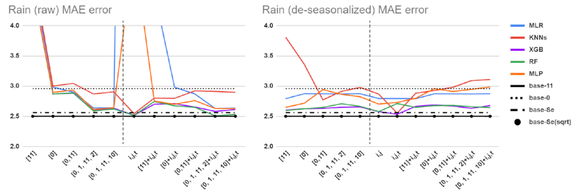
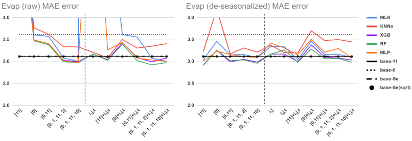
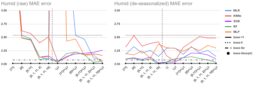
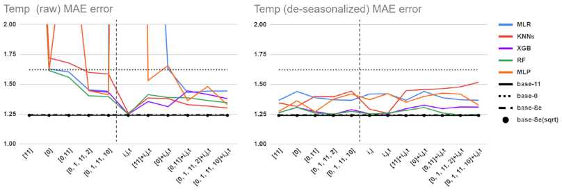
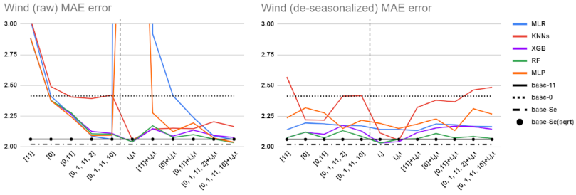
5.1. Performance Comparisons for Different Baselines, Feature Sets, and Preprocessing Methods

Figure 6 gives residual plots and R 2 values for the three baselines base-11, base-0, and base-Se(sqrt) for the five climatic parameters (base-Se is not shown, but strongly resembles base-Se(sqrt)). As seen in the figure, Base-Se(sqrt) gives the most accurate estimations across all parameters (predictions lie closer to the 45 line), as well as giving larger R 2 values. Indeed, the R 2 performance for base-Se(sqrt) is almost perfect, with all values over 0.96.
Figure 7, Figure 8, Figure 9, Figure 10 and Figure 11 summarize the MAE results for models trained using different feature sets for each of the climatic parameters. The corresponding RMSE values were also generated, but since they closely resemble the MAE results, they are omitted here. Each figure contains two line graphs for raw and de-seasonalized data sets, respectively. For the raw data, the [i,j] feature set performed very badly, so we omitted these results from the figures to avoid stretching the vertical scale. In addition, the base-11 baseline was above the vertical scale for all parameters except rainfall, and is not shown.
Of the four baselines, base-Se(sqrt) is always the best, followed by base-Se, base-0, and base-11, in that order. In fact, Base-Se(sqrt) is also better than all ML tools for all parameters and feature sets, except evaporation for a few feature sets.
Next, comparison between raw-based and de-seasonalized-based predictions shows that de-seasonalizing tends to stabilize the performance, so that it is less dependent on the feature set used. If the feature set contains [0], then de-seasonalizing makes little difference. De-seasonalizing does not always improve the feature sets’ performances, as will be discussed in more detail below.
A comparison of feature sets shows that the feature sets [i,j,t],[11,i,j,t], and [0,11,i,j,t] are consistently the best performers, both for raw-based and de-seasonalized-based predictions. In our detailed performance analysis below, we focus on these three feature sets.
It is significant that the above observations apply consistently to all five parameters, which suggests that the same observations can generalize to other climatic parameters.

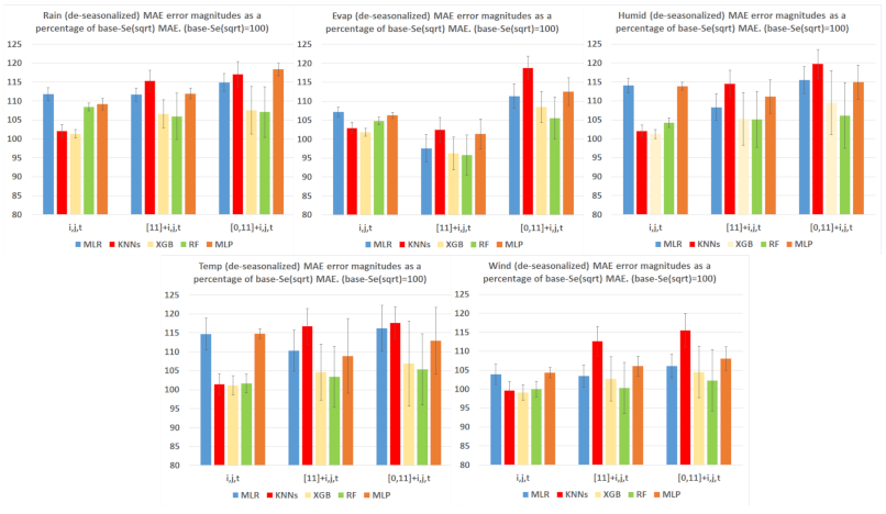
5.2. Detailed Comparison of ML Tools and Feature Sets

Figure 12 and Figure 13 show the percentage error reductions for different ML algorithms for the 5 climatic parameters, using raw and de-seasonalized data, respectively. Only the three best feature sets are represented, namely i,j,t, [11]+i,j,t, and [0,11]+i,j,t. In the figures, the 100 % level corresponds to the Base-Se(sqrt) MAE error: so, for example, the MLR value of 120% for rain (raw) with feature set [0,11] + i,j,t indicates that the MAE error for MLR is 1.2 times the corresponding Base-Se(sqrt) error. Error bars in the figures correspond to ± 2 standard deviations, and were computed using the jackknife procedure described in Section 4.4.2, using the different ML methods and the Base-Se(sqrt) baseline.
For raw-based predictions, Figure 12 shows that the KNN, XGB, and RF algorithms typically attain between 100 and 110% of base-Se(sqrt) across all parameters, while MLR and MLP exceed 125% in several cases. For evaporation with the [11]+i,j,t feature set and for wind with the i,j,t feature set, the KNN XGB and RF algorithms are slightly better than base-Se(sqrt), but the error bars show that this relative improvement is not statistically significant.
For deseasonalized-based predictions, the accuracy of XGB and RF is nearly the same as for raw-based, but KNN performance is degraded by up to 10%. The errors for MLR and MLP are reduced to below 115%, but still tend to be 5–10% higher than errors for XGB and RF.
For all parameters except evaporation, the ML methods of KNN, XGB, and RF applied to the feature set i,j,t give the best performance on both raw and de-seasonalized data. This implies that (surprisingly) including lag-based features actually worsens prediction accuracy for these parameters. It is also surprising that the most and least sophisticated methods (MLR and MLP) have similar (and sub-optimal) performance in most cases.

5.3. Data Shuffling

In Section 1, we mentioned that several references shuffle the image sequences. In order to gauge the effects of this shuffling, we used RF with features set [11]+i,j,t to predict all climatic parameters with both shuffled and unshuffled data. For both shuffled and unshuffled data, 156 of the 216 total 12-month sequences were used for training and the rest for testing. The unshuffled data used the first 156 sequences for training and rest for testing, as described in Section 4.2, while the shuffled data took 156 sequences randomly from the entire dataset, thus producing overlap between training and testing sequences. Results showed that MAE obtained from shuffled data was 2-10% lower than from unshuffled data, due to data leakage.

6. Discussion

The results demonstrate that when doing seasonal parameter prediction on monthly time scales, it is important to use a well-motivated simple baseline, e.g., a statistical estimator computed from the source data. This finding is consistent with the points made in [9]. Baselines that depend on lags do not perform as well. Furthermore, a simple same-month average baseline which does not take into account the statistical properties of MAE cannot match the performance of baseline that is designed to estimate median values, which in theory will minimize MAE. For the seasonal parameters we tested, a carefully designed statistical estimator outperforms even highly sophisticated ML models. This finding raises concerns about positive results reported in previous papers that fail to supply statistical baselines.
The results also show that care must be taken in selecting seasonal features as inputs. In the literature, same month previous year (corresponding to our feature [0]) is commonly used [13,17,19,20,24,25,27,28,44,49,51,58,60,62,67]. However, we found that using [0] scarcely outperforms base-0, and is much worse than base-Se(sqrt). Indeed, we found that time stamp t (where t runs from 0 to 11) gave much better results, although it is rarely used in the literature. In addition, using both features typically gave worse performance than using t only.
Aside from using seasonal features, another way to account for seasonality is to de-seasonalize the input data by subtracting monthly averages. The results show that de-seasonalization tends to reduce model complexity: for example, when data is de-seasonalized, then feature [0] becomes unnecessary. However, whether or not de-seasonalization lowers the error depends which algorithm and which features set is used. For example, the best-performing feature-algorithm combinations in our study used i,j,t with RF, or XGB, and for these combinations de-seasonalization of inputs made no difference. We conclude that appropriate feature and algorithm selection has more of an effect on performance than de-seasonalization.
A study similar to ours may be found in [45], in which base-Se is used to standardize the performance of different ML models in predicting 1–6 months ahead rainfall using past rainfall, temperature, and climate index. Compared to base-Se, the following ML algorithms had worse performance: MLR, RF, support vector machine (SVM), artificial neural network (ANN), long short term memory neural networks (LSTM), and convolutional LSTM (ConvLSTM). It follows that including additional climatic parameters as features and doing joint prediction may yield no benefits. Only when the authors used wavelets during pre-processing did their accuracy improve. Even with wavelets, the basic MLR model gave results that nearly matched a sophisticated LSTM model (no error bars for the difference are given, so it is impossible to tell whether there is a significant difference).
For the climatic parameters that were examined in this paper, using previous month (denoted as feature [11]) was not effective, and could even degrade predictive performance when added. However, this conclusion is not applicable to other parameters such as groundwater [7,57], which involves conditions that last over multiple months. The slight improvements seen when adding [11] to evaporation may be due to this effect.
Unlike most prior research in this area, we established the significance of differences in predictive performance between ML methods using error bars that were calculated using statistically rigorous jackknife estimates. The error bars for differences between MAE values for different estimation methods were much smaller than error bars on the MAE values themselves (such as those calculated in [45]). The jackknife methods employed are quite general, and can be used for other ML applications.
Finally, we established that images used for training and testing must be strictly separated and timed. Shuffling of image sequences, which has been employed in some prior research, leads to data leakage, which produces artificial reductions of prediction errors.

7. Conclusions

In this paper, we studied the application of machine learning to the prediction of seasonal climatic parameters on a monthly basis. Our conclusions may be briefly summarized as follows. First, a well-thought out baseline based on a simple statistical estimator will often outperform all ML models. Hence, studies of ML prediction algorithms that do not provide a baseline comparison are not sufficiently demonstrating the effectiveness of the algorithms. Second, the use of time stamp (i.e., month index) as a feature can replace de-seasonalization, and often yields better results than lags (i.e., previous month, or same month previous year). Third, we have demonstrated that jackknife estimation can be used to calculate error bars on algorithms’ relative performance, which until now have not been generally reported in the literature. Fourth, we have shown that the practice of data shuffling produces error estimates that are artificially lowered. The methods we have used are quite general, and can be readily applied to other situations. The fact that our results are consistent over five widely different climatic parameters suggests that similar results may be expected for other climatic parameters measured on other regions. This conclusion is reinforced by the fact that similar results have been observed in another study of rainfall conducted in China [45].
In the current research, we have considered only single parameter prediction, using local spatio-temporal based features. For future work, we may apply similar methods to predictions based on other features. Reference [45] for instance shows that using wavelets can lead to better predictions—the question remains whether ML applied to these features can bring significant improvements, or whether simple statistics are sufficient.
Another possibility for future research is the application of deep learning. However, since most monthly datasets available are not large, deep learning may be of limited applicability for monthly prediction. Furthermore, the authors of [45] found that deep learning did not significantly improve on multi-linear regression for monthly rainfall prediction. Nonetheless, since the field of deep learning is developing rapidly, future techniques may produce algorithms that perform well even on datasets of limited size.

Author Contributions

Conceptualization, M.G., A.B. and E.A.H.; methodology, M.G. and E.A.H.; software, E.A.H.; validation, M.G. and C.T.; formal analysis, C.T. and E.A.H.; computing resources, M.G., M.V., and A.B.; writing—original draft preparation, E.A.H.; writing—review and editing, M.G., M.V., C.T. and A.B.; visualization, M.G., C.T. and E.A.H.; supervision, M.G., C.T. and A.B.; funding acquisition, M.G. and M.V. All authors have read and agreed to the published version of the manuscript.

Funding

E.A.H. acknowledges financial support from the South African National Research Foundation (NRF CSUR Grant Number 121291 for the HIPPO project) and from the Telkom-Openserve-Aria Technologies Center of Excellence at the Department of Computer Science of the University of the Western Cape.

Data Availability Statement

Data available in a publicly accessible repository The data presented in this study are openly available in the GES DISC repository at doi:10.5067/5NHC22T9375G.

Acknowledgments

This work made use of the Meerkat Cluster (http://docs.meerkat.uwc.ac.za (accessed on 16 April 2021)) provided by the University of the Western Cape’s eResearch Office (https://eresearch.uwc.ac.za (accessed on 16 April 2021)).

Conflicts of Interest

The authors declare no conflict of interest.

Abbreviations

The following abbreviations are used in this manuscript:
MLMachine learning
ANNsArtificial neural networks
Base-0,…,base-11Baseline estimators based on previous lags (see Section 4.4.3)
Base-SeSeasonal baseline computed from same-month averages (see Section 4.4.3)
Base-Se(sqrt)Seasonal baseline computed from regularized same-month averages
(see Section 4.4.3)
CNNsConvolution neural networks
LSTMsLong short term memory
ConvLSTMsConvolutions layers with Long short term memory
MLPMultilayer perceptron
RFRandom forest
SVMsSupport vector machines
XGBExtreme gradient boosting
MLRMulti linear regression
KNNK-nearest neighbour
RMSERoot mean square error
MAEMean absolute error
RainRainfall
TempTemperature
EvapEvaporation
HumidHumidity
FEWS NETFamine Early Warning Systems Network
FLDASFEWS NET Land Data Assimilation System

References

  1. Miller, H.J.; Goodchild, M.F. Data-driven geography. GeoJournal 2015, 80, 449–461. [Google Scholar] [CrossRef]
  2. Hey, T.; Tansley, S.; Tolle, K. The Fourth Paradigm: Data-Intensive Scientific Discovery; Microsoft research Redmond: Redmond, WA, USA, 2009; Volume 1. [Google Scholar]
  3. Manyika, J.; Chui, M.; Brown, B.; Bughin, J.; Dobbs, R.; Roxburgh, C.; Hung Byers, A. Big Data: The Next Frontier for Innovation, Competition, and Productivity; McKinsey Global Institute: New York, NY, USA, 2011. [Google Scholar]
  4. Kitchin, R. Big Data, new epistemologies and paradigm shifts. Big Data Soc. 2014, 1, 2053951714528481. [Google Scholar] [CrossRef] [Green Version]
  5. Ardabili, S.; Mosavi, A.; Dehghani, M.; Várkonyi-Kóczy, A.R. Deep learning and machine learning in hydrological processes climate change and earth systems a systematic review. In International Conference on Global Research and Education; Springer: Berlin/Heidelberg, Germany, 2019; pp. 52–62. [Google Scholar]
  6. Monteleoni, C.; Schmidt, G.A.; McQuade, S. Climate informatics: Accelerating discovering in climate science with machine learning. Comput. Sci. Eng. 2013, 15, 32–40. [Google Scholar] [CrossRef]
  7. Buontempo, C.; Hewitt, C.D.; Doblas-Reyes, F.J.; Dessai, S. Climate service development, delivery and use in Europe at monthly to inter-annual timescales. Clim. Risk Manag. 2014, 6, 1–5. [Google Scholar] [CrossRef] [Green Version]
  8. Steinert, M.; Leifer, L. Scrutinizing Gartner’s hype cycle approach. In Proceedings of the Picmet 2010 Technology Management for Global Economic Growth, Phuket, Thailand, 18–22 July 2010; IEEE: Piscataway, NJ, USA, 2010; pp. 1–13. [Google Scholar]
  9. Dacrema, M.F.; Cremonesi, P.; Jannach, D. Are we really making much progress? A worrying analysis of recent neural recommendation approaches. In Proceedings of the 13th ACM Conference on Recommender Systems, Copenhagen, Denmark, 16–20 September 2019; pp. 101–109. [Google Scholar]
  10. Lin, J. The neural hype and comparisons against weak baselines. In ACM SIGIR Forum; ACM: New York, NY, USA, 2019; Volume 52, pp. 40–51. [Google Scholar]
  11. Hussein, E.A.; Ghaziasgar, M.; Thron, C. Regional Rainfall Prediction Using Support Vector Machine Classification of Large-Scale Precipitation Maps. arXiv 2020, arXiv:2007.15404. [Google Scholar]
  12. Ludewig, M.; Jannach, D. Evaluation of session-based recommendation algorithms. User Model. User-Adapt. Interact. 2018, 28, 331–390. [Google Scholar] [CrossRef] [Green Version]
  13. Cristian, M. Average monthly rainfall forecast in Romania by using K-nearest neighbors regression. Analele Univ. Constantin Brâncuşi Din Târgu Jiu Ser. Econ. 2018, 1, 5–12. [Google Scholar]
  14. Karimi, H.A. Big Data: Techniques and Technologies in Geoinformatics; CRC Press: Boca Raton, FL, USA, 2014. [Google Scholar]
  15. Armstrong, T.G.; Moffat, A.; Webber, W.; Zobel, J. Improvements that do not add up: Ad-hoc retrieval results since 1998. In Proceedings of the 18th ACM conference on Information and knowledge management, Hong Kong, China, 2–6 November 2009; pp. 601–610. [Google Scholar]
  16. Du, Y.; Berndtsson, R.; An, D.; Zhang, L.; Yuan, F.; Uvo, C.B.; Hao, Z. Multi-Space Seasonal Precipitation Prediction Model Applied to the Source Region of the Yangtze River, China. Water 2019, 11, 2440. [Google Scholar] [CrossRef] [Green Version]
  17. Lakshmaiah, K.; Krishna, S.M.; Reddy, B.E. Application of referential ensemble learning techniques to predict the density of rainfall. In Proceedings of the 2016 International Conference on Electrical, Electronics, Communication, Computer and Optimization Techniques (ICEECCOT), Mysuru, India, 9–10 December 2016; IEEE: Piscataway, NJ, USA, 2016; pp. 233–237. [Google Scholar]
  18. Lee, J.; Kim, C.G.; Lee, J.E.; Kim, N.W.; Kim, H. Application of artificial neural networks to rainfall forecasting in the Geum River basin, Korea. Water 2018, 10, 1448. [Google Scholar] [CrossRef] [Green Version]
  19. Beheshti, Z.; Firouzi, M.; Shamsuddin, S.M.; Zibarzani, M.; Yusop, Z. A new rainfall forecasting model using the CAPSO algorithm and an artificial neural network. Neural Comput. Appl. 2016, 27, 2551–2565. [Google Scholar] [CrossRef]
  20. Duong, T.A.; Bui, M.D.; Rutschmann, P. A comparative study of three different models to predict monthly rainfall in Ca Mau, Vietnam. In Wasserbau-Symposium Graz 2018. Wasserwirtschaft–Innovation aus Tradition. Tagungsband. Beiträge Zum 19; Gemeinschafts-Symposium der Wasserbau-Institute TU München, TU Graz und ETH Zürich: Graz, Austria, 2018; p. Paper–G5. [Google Scholar]
  21. Gao, L.; Wei, F.; Yan, Z.; Ma, J.; Xia, J. A Study of Objective Prediction for Summer Precipitation Patterns Over Eastern China Based on a Multinomial Logistic Regression Model. Atmosphere 2019, 10, 213. [Google Scholar] [CrossRef] [Green Version]
  22. Mishra, N.; Kushwaha, A. Rainfall Prediction using Gaussian Process Regression Classifier. Int. J. Adv. Res. Comput. Eng. Technol. (IJARCET) 2019, 8. [Google Scholar]
  23. Aguasca-Colomo, R.; Castellanos-Nieves, D.; Méndez, M. Comparative analysis of rainfall prediction models using machine learning in islands with complex orography: Tenerife Island. Appl. Sci. 2019, 9, 4931. [Google Scholar] [CrossRef] [Green Version]
  24. Sulaiman, J.; Wahab, S.H. Heavy rainfall forecasting model using artificial neural network for flood prone area. In IT Convergence and Security 2017; Springer: Berlin/Heidelberg, Germany, 2018; pp. 68–76. [Google Scholar]
  25. Chhetri, M.; Kumar, S.; Pratim Roy, P.; Kim, B.G. Deep BLSTM-GRU Model for Monthly Rainfall Prediction: A Case Study of Simtokha, Bhutan. Remote Sens. 2020, 12, 3174. [Google Scholar] [CrossRef]
  26. Bojang, P.O.; Yang, T.C.; Pham, Q.B.; Yu, P.S. Linking Singular Spectrum Analysis and Machine Learning for Monthly Rainfall Forecasting. Appl. Sci. 2020, 10, 3224. [Google Scholar] [CrossRef]
  27. Canchala, T.; Alfonso-Morales, W.; Carvajal-Escobar, Y.; Cerón, W.L.; Caicedo-Bravo, E. Monthly Rainfall Anomalies Forecasting for Southwestern Colombia Using Artificial Neural Networks Approaches. Water 2020, 12, 2628. [Google Scholar] [CrossRef]
  28. Mehr, A.D.; Nourani, V.; Khosrowshahi, V.K.; Ghorbani, M.A. A hybrid support vector regression–firefly model for monthly rainfall forecasting. Int. J. Environ. Sci. Technol. 2019, 16, 335–346. [Google Scholar] [CrossRef]
  29. Shi, X.; Chen, Z.; Wang, H.; Yeung, D.; Wong, W.; Woo, W.C. Convolutional LSTM Network: A Machine Learning Approach for Precipitation Nowcasting. arXiv 2015, arXiv:1506.04214. [Google Scholar]
  30. Manandhar, S.; Dev, S.; Lee, Y.H.; Meng, Y.S.; Winkler, S. A data-driven approach for accurate rainfall prediction. IEEE Trans. Geosci. Remote Sens. 2019, 57, 9323–9331. [Google Scholar] [CrossRef] [Green Version]
  31. Jing, J.; Li, Q.; Peng, X. MLC-LSTM: Exploiting the Spatiotemporal Correlation between Multi-Level Weather Radar Echoes for Echo Sequence Extrapolation. Sensors 2019, 19, 3988. [Google Scholar] [CrossRef] [Green Version]
  32. Sato, R.; Kashima, H.; Yamamoto, T. Short-term precipitation prediction with skip-connected prednet. In International Conference on Artificial Neural Networks; Springer: Berlin/Heidelberg, Germany, 2018; pp. 373–382. [Google Scholar]
  33. Ayzel, G.; Heistermann, M.; Sorokin, A.; Nikitin, O.; Lukyanova, O. All convolutional neural networks for radar-based precipitation nowcasting. Procedia Comput. Sci. 2019, 150, 186–192. [Google Scholar] [CrossRef]
  34. Singh, S.; Sarkar, S.; Mitra, P. A deep learning based approach with adversarial regularization for Doppler weather radar ECHO prediction. In Proceedings of the 2017 IEEE International Geoscience and Remote Sensing Symposium (IGARSS), Fort Worth, TX, USA, 23–28 July 2017; IEEE: Piscataway, NJ, USA, 2017; pp. 5205–5208. [Google Scholar]
  35. Chen, L.; Cao, Y.; Ma, L.; Zhang, J. A Deep Learning Based Methodology for Precipitation Nowcasting with Radar. Earth Space Sci. 2020, 7, e2019EA000812. [Google Scholar] [CrossRef] [Green Version]
  36. Tran, Q.K.; Song, S.k. Computer vision in precipitation nowcasting: Applying image quality assessment metrics for training deep neural networks. Atmosphere 2019, 10, 244. [Google Scholar] [CrossRef] [Green Version]
  37. Shi, E.; Li, Q.; Gu, D.; Zhao, Z. Convolutional Neural Networks Applied on Weather Radar Echo Extrapolation. DEStech Trans. Comput. Sci. Eng. 2017. [Google Scholar] [CrossRef] [Green Version]
  38. Castro, R.; Souto, Y.M.; Ogasawara, E.; Porto, F.; Bezerra, E. STConvS2S: Spatiotemporal Convolutional Sequence to Sequence Network for weather forecasting. Neurocomputing 2020, 426, 285–298. [Google Scholar] [CrossRef]
  39. Wang, Y.; Long, M.; Wang, J.; Gao, Z.; Philip, S.Y. Predrnn: Recurrent neural networks for predictive learning using spatiotemporal lstms. Adv. Neural Inf. Process. Syst. 2017, 879–888. [Google Scholar]
  40. Tran, Q.K.; Song, S.k. Multi-Channel Weather Radar Echo Extrapolation with Convolutional Recurrent Neural Networks. Remote Sens. 2019, 11, 2303. [Google Scholar] [CrossRef] [Green Version]
  41. Zhang, P.; Jia, Y.; Gao, J.; Song, W.; Leung, H.K. Short-term rainfall forecasting using multi-layer perceptron. IEEE Trans. Big Data 2018, 6, 93–106. [Google Scholar] [CrossRef]
  42. Oswal, N. Predicting rainfall using machine learning techniques. arXiv 2019, arXiv:1910.13827. [Google Scholar]
  43. Balamurugan, M.; Manojkumar, R. Study of short term rain forecasting using machine learning based approach. Wirel. Netw. 2019, 1–6. [Google Scholar] [CrossRef]
  44. Nourani, V.; Uzelaltinbulat, S.; Sadikoglu, F.; Behfar, N. Artificial intelligence based ensemble modeling for multi-station prediction of precipitation. Atmosphere 2019, 10, 80. [Google Scholar] [CrossRef] [Green Version]
  45. Xu, L.; Chen, N.; Zhang, X.; Chen, Z. A data-driven multi-model ensemble for deterministic and probabilistic precipitation forecasting at seasonal scale. Clim. Dyn. 2020, 54, 1–20. [Google Scholar] [CrossRef]
  46. Mehdizadeh, S.; Behmanesh, J.; Khalili, K. New approaches for estimation of monthly rainfall based on GEP-ARCH and ANN-ARCH hybrid models. Water Resour. Manag. 2018, 32, 527–545. [Google Scholar] [CrossRef]
  47. Shenify, M.; Danesh, A.S.; Gocić, M.; Taher, R.S.; Wahab, A.W.A.; Gani, A.; Shamshirband, S.; Petković, D. Precipitation estimation using support vector machine with discrete wavelet transform. Water Resour. Manag. 2016, 30, 641–652. [Google Scholar] [CrossRef]
  48. Banadkooki, F.B.; Ehteram, M.; Ahmed, A.N.; Fai, C.M.; Afan, H.A.; Ridwam, W.M.; Sefelnasr, A.; El-Shafie, A. Precipitation forecasting using multilayer neural network and support vector machine optimization based on flow regime algorithm taking into account uncertainties of soft computing models. Sustainability 2019, 11, 6681. [Google Scholar] [CrossRef] [Green Version]
  49. Haidar, A.; Verma, B. Monthly rainfall forecasting using one-dimensional deep convolutional neural network. IEEE Access 2018, 6, 69053–69063. [Google Scholar] [CrossRef]
  50. Zhan, C.; Wu, F.; Wu, Z.; Chi, K.T. Daily Rainfall Data Construction and Application to Weather Prediction. In Proceedings of the 2019 IEEE International Symposium on Circuits and Systems (ISCAS), Hokkaido, Japan, 26–29 May 2019; IEEE: Piscataway, NJ, USA, 2019; pp. 1–5. [Google Scholar]
  51. Weesakul, U.; Kaewprapha, P.; Boonyuen, K.; Mark, O. Deep learning neural network: A machine learning approach for monthly rainfall forecast, case study in eastern region of Thailand. Eng. Appl. Sci. Res. 2018, 45, 203–211. [Google Scholar]
  52. Chattopadhyay, A.; Hassanzadeh, P.; Pasha, S. Predicting clustered weather patterns: A test case for applications of convolutional neural networks to spatio-temporal climate data. Sci. Rep. 2020, 10, 1–13. [Google Scholar] [CrossRef]
  53. Patel, M.; Patel, A.; Ghosh, D. Precipitation nowcasting: Leveraging bidirectional lstm and 1d cnn. arXiv 2018, arXiv:1810.10485. [Google Scholar]
  54. Zhuang, W.; Ding, W. Long-lead prediction of extreme precipitation cluster via a spatiotemporal convolutional neural network. In Proceedings of the 6th International Workshop on Climate Informatics: CI, Boulder, CO, USA, 22–23 September 2016. [Google Scholar]
  55. Boonyuen, K.; Kaewprapha, P.; Srivihok, P. Daily rainfall forecast model from satellite image using Convolution neural network. In Proceedings of the 2018 IEEE International Conference on Information Technology, Bhubaneswar, India, 19–21 December 2018; pp. 1–7. [Google Scholar]
  56. Boonyuen, K.; Kaewprapha, P.; Weesakul, U.; Srivihok, P. Convolutional Neural Network Inception-v3: A Machine Learning Approach for Leveling Short-Range Rainfall Forecast Model from Satellite Image. In International Conference on Swarm Intelligence; Springer: Berlin/Heidelberg, Germany, 2019; pp. 105–115. [Google Scholar]
  57. Hussein, E.A.; Thron, C.; Ghaziasgar, M.; Bagula, A.; Vaccari, M. Groundwater Prediction Using Machine-Learning Tools. Algorithms 2020, 13, 300. [Google Scholar] [CrossRef]
  58. Aswin, S.; Geetha, P.; Vinayakumar, R. Deep learning models for the prediction of rainfall. In Proceedings of the 2018 International Conference on Communication and Signal Processing (ICCSP), Tamilnadu, India, 3–5 April 2018; IEEE: Piscataway, NJ, USA, 2018; pp. 0657–0661. [Google Scholar]
  59. Amiri, M.A.; Amerian, Y.; Mesgari, M.S. Spatial and temporal monthly precipitation forecasting using wavelet transform and neural networks, Qara-Qum catchment, Iran. Arab. J. Geosci. 2016, 9, 421. [Google Scholar] [CrossRef]
  60. Abbot, J.; Marohasy, J. Forecasting Monthly Rainfall in the Western Australian Wheat-Belt up to 18-Months in Advance Using Artificial Neural Networks. In Australasian Joint Conference on Artificial Intelligence; Springer: Berlin/Heidelberg, Germany, 2016; pp. 71–87. [Google Scholar]
  61. Damavandi, H.G.; Shah, R. A Learning Framework for An Accurate Prediction of Rainfall Rates. arXiv 2019, arXiv:1901.05885. [Google Scholar]
  62. Abbot, J.; Marohasy, J. Application of artificial neural networks to forecasting monthly rainfall one year in advance for locations within the Murray Darling basin, Australia. Int. J. Sustain. Dev. Plan. 2017, 12, 1282–1298. [Google Scholar] [CrossRef] [Green Version]
  63. Mohamadi, S.; Ehteram, M.; El-Shafie, A. Accuracy enhancement for monthly evaporation predicting model utilizing evolutionary machine learning methods. Int. J. Environ. Sci. Technol. 2020, 17, 3373–3396. [Google Scholar] [CrossRef]
  64. Delleur, J.W.; Kavvas, M.L. Stochastic models for monthly rainfall forecasting and synthetic generation. J. Appl. Meteorol. 1978, 17, 1528–1536. [Google Scholar] [CrossRef] [Green Version]
  65. Barnett, A.G.; Baker, P.; Dobson, A. Analysing seasonal data. R J. 2012, 4, 5–10. [Google Scholar] [CrossRef] [Green Version]
  66. Nielsen, A. Practical Time Series Analysis: Prediction with Statistics and Machine Learning; O’Reilly: Newton, MA, USA, 2020. [Google Scholar]
  67. Kumar, D.; Singh, A.; Samui, P.; Jha, R.K. Forecasting monthly precipitation using sequential modelling. Hydrol. Sci. J. 2019, 64, 690–700. [Google Scholar] [CrossRef]
  68. Ramsundram, N.; Sathya, S.; Karthikeyan, S. Comparison of decision tree based rainfall prediction model with data driven model considering climatic variables. Irrig. Drain. Syst. Eng. 2016. [Google Scholar] [CrossRef] [Green Version]
  69. Sardeshpande, K.D.; Thool, V.R. Rainfall Prediction: A Comparative Study of Neural Network Architectures. In Emerging Technologies in Data Mining and Information Security; Springer: Berlin/Heidelberg, Germany, 2019; pp. 19–28. [Google Scholar]
  70. Shi, X.; Gao, Z.; Lausen, L.; Wang, H.; Yeung, D.Y.; Wong, W.k.; Woo, W.c. Deep learning for precipitation nowcasting: A benchmark and a new model. Adv. Neural Inf. Process. Syst. 2017, 5617–5627. [Google Scholar]
  71. McNally, A. FLDAS Noah Land Surface Model L4 Global Monthly 0.1 × 0.1 degree (MERRA-2 and CHIRPS). Atmos. Compos. Water Energy Cycles Clim. Var. 2018. [Google Scholar] [CrossRef]
  72. Loeser, C.; Rui, H.; Teng, W.L.; Ostrenga, D.M.; Wei, J.C.; Mcnally, A.L.; Jacob, J.P.; Meyer, D.J. Famine Early Warning Systems Network (FEWS NET) Land Data Assimilation System (LDAS) and Other Assimilated Hydrological Data at NASA GES DISC. In Proceedings of the 100th American Meteorological Society Annual Meeting, St. Boston, MA, USA, 12–16 January 2020. [Google Scholar]
  73. Nematchoua, M.K. A study on outdoor environment and climate change effects in Madagascar. J. Build. Sustain. 2017, 1, 12. [Google Scholar]
  74. Tadross, M.; Randriamarolaza, L.; Rabefitia, Z.; Zheng, K. Climate Change in Madagascar; Recent Past and Future; World Bank: Washington, DC, USA, 2008; Volume 18. [Google Scholar]
  75. Szabó, A.; Raveloson, A.; Székely, B. Landscape evolution and climate in Madagascar: Lavakization in the light of archive precipitation data. Cuad. Investig. GeogrÁFica/Geogr. Res. Lett. 2015, 41, 181–204. [Google Scholar] [CrossRef] [Green Version]
  76. Harvey, C.A.; Rakotobe, Z.L.; Rao, N.S.; Dave, R.; Razafimahatratra, H.; Rabarijohn, R.H.; Rajaofara, H.; MacKinnon, J.L. Extreme vulnerability of smallholder farmers to agricultural risks and climate change in Madagascar. Philos. Trans. R. Soc. B Biol. Sci. 2014, 369, 20130089. [Google Scholar] [CrossRef] [Green Version]
  77. Ingram, J.C.; Dawson, T.P. Climate change impacts and vegetation response on the island of Madagascar. Philos. Trans. R. Soc. A Math. Phys. Eng. Sci. 2005, 363, 55–59. [Google Scholar] [CrossRef]
  78. Sanchez-Pi, N.; Marti, L.; Abreu, A.; Bernard, O.; de Vargas, C.; Eveillard, D.; Maass, A.; Marquet, P.A.; Sainte-Marie, J.; Salomon, J.; et al. Artificial Intelligence, Machine Learning and Modeling for Understanding the Oceans and Climate Change. In NeurIPS 2020 Workshop-Tackling Climate Change with Machine Learning; 2020; Available online: https://hal.archives-ouvertes.fr/hal-03138712 (accessed on 19 April 2021).
  79. Stein, A.L. Artificial Intelligence and Climate Change. Yale J. Reg. 2020, 37, 890. [Google Scholar]
  80. Abudu, S.; Cui, C.; King, J.P.; Moreno, J.; Bawazir, A.S. Modeling of daily pan evaporation using partial least squares regression. Sci. China Technol. Sci. 2011, 54, 163–174. [Google Scholar] [CrossRef]
  81. Pinheiro, A.; Vidakovic, B. Estimating the square root of a density via compactly supported wavelets. Comput. Stat. Data Anal. 1997, 25, 399–415. [Google Scholar] [CrossRef]
  82. Qiu, M.; Zhao, P.; Zhang, K.; Huang, J.; Shi, X.; Wang, X.; Chu, W. A short-term rainfall prediction model using multi-task convolutional neural networks. In Proceedings of the 2017 IEEE International Conference on Data Mining (ICDM), New Orleans, LA, USA, 18–21 November 2017; IEEE: Piscataway, NJ, USA, 2017; pp. 395–404. [Google Scholar]
  83. Cramer, S.; Kampouridis, M.; Freitas, A.A.; Alexandridis, A.K. An extensive evaluation of seven machine learning methods for rainfall prediction in weather derivatives. Expert Syst. Appl. 2017, 85, 169–181. [Google Scholar] [CrossRef] [Green Version]
  84. Cao, Y.; Li, Q.; Shan, H.; Huang, Z.; Chen, L.; Ma, L.; Zhang, J. Precipitation Nowcasting with Star-Bridge Networks. arXiv 2019, arXiv:1907.08069. [Google Scholar]
  85. Klein, B.; Wolf, L.; Afek, Y. A dynamic convolutional layer for short range weather prediction. In Proceedings of the IEEE Conference on Computer Vision and Pattern Recognition, Boston, MA, USA, 7–12 June 2015; pp. 4840–4848. [Google Scholar]
  86. Mukhopadhyay, A.; Shukla, B.P.; Mukherjee, D.; Chanda, B. A novel neural network based meteorological image prediction from a given sequence of images. In Proceedings of the 2011 Second International Conference on Emerging Applications of Information Technology, Kolkata, India, 19–20 February 2011; IEEE: Piscataway, NJ, USA, 2011; pp. 202–205. [Google Scholar]
  87. Vandekerckhove, J.; Matzke, D.; Wagenmakers, E.J. Model comparison and the principle of parsimony. In Oxford Handbook of Computational and Mathematical Psychology; Oxford University Press: Oxford, UK, 2015; pp. 300–319. [Google Scholar]
  88. Dash, Y.; Mishra, S.K.; Panigrahi, B.K. Rainfall prediction for the Kerala state of India using artificial intelligence approaches. Comput. Electr. Eng. 2018, 70, 66–73. [Google Scholar] [CrossRef]
  89. Purushotham, S.; Meng, C.; Che, Z.; Liu, Y. Benchmarking deep learning models on large healthcare datasets. J. Biomed. Inform. 2018, 83, 112–134. [Google Scholar] [CrossRef] [PubMed]
  90. Leming, M.; Górriz, J.M.; Suckling, J. Ensemble deep learning on large, mixed-site fMRI datasets in autism and other tasks. arXiv 2020, arXiv:2002.07874. [Google Scholar] [CrossRef] [PubMed] [Green Version]
  91. Chen, X.W.; Lin, X. Big data deep learning: Challenges and perspectives. IEEE Access 2014, 2, 514–525. [Google Scholar] [CrossRef]
  92. Zhang, Q.; Yang, L.T.; Chen, Z.; Li, P. A survey on deep learning for big data. Inf. Fusion 2018, 42, 146–157. [Google Scholar] [CrossRef]
  93. Buitinck, L.; Louppe, G.; Blondel, M.; Pedregosa, F.; Mueller, A.; Grisel, O.; Niculae, V.; Prettenhofer, P.; Gramfort, A.; Grobler, J.; et al. API Design for machine learning software: Experiences from the scikit-learn project. arXiv 2013, arXiv:1309.0238. [Google Scholar]
  94. Stigler, S.M. Studies in the History of Probability and Statistics. XXXII: Laplace, Fisher, and the discovery of the concept of sufficiency. Biometrika 1973, 60, 439–445. [Google Scholar] [CrossRef]
  95. Willmott, C.J.; Matsuura, K. Advantages of the mean absolute error (MAE) over the root mean square error (RMSE) in assessing average model performance. Clim. Res. 2005, 30, 79–82. [Google Scholar] [CrossRef]
  96. Chai, T.; Draxler, R.R. Root mean square error (RMSE) or mean absolute error (MAE)?–Arguments against avoiding RMSE in the literature. Geosci. Model Dev. 2014, 7, 1247–1250. [Google Scholar] [CrossRef] [Green Version]
  97. Brassington, G. Mean absolute error and root mean square error: Which is the better metric for assessing model performance? Egu Gen. Assem. Conf. Abstr. 2017, 19, 3574. [Google Scholar]
  98. Efron, B.; Stein, C. The jackknife estimate of variance. Ann. Stat. 1981, 9, 586–596. [Google Scholar] [CrossRef]
Figure 1. A sample full image of the rainfall dataset used in this research [72]. Color scale indicates normalized rainfall intensities.
Atmosphere 12 00539 g001
Figure 2. Images showing normalized values of five climatic parameters of Madagascar used in this study (left to right): rainfall (Rain), evaporation (Evap), humidity (Humid), temperature (Temp), and wind.
Atmosphere 12 00539 g002
Figure 3. Flowchart showing the implementation process.
Atmosphere 12 00539 g003
Figure 4. Pre-processed rainfall images (compare first image in Figure 2): raw image (left) and de-seasonalized image (right).
Atmosphere 12 00539 g004
Figure 5. Overview of dataset preparation: Notation for same-pixel features used in image prediction.
Atmosphere 12 00539 g005
Figure 6. Residual plots and R 2 values for three proposed baselines on five different parameters. The scatter plots show 5000 randomly-selected point for each baseline, for each parameter.
Atmosphere 12 00539 g006
Figure 7. MAE for rainfall predictions with different feature sets, for raw and de-seasonalized data sets.
Atmosphere 12 00539 g007
Figure 8. MAE for evaporation predictions with different feature sets, for raw and de-seasonalized data sets.
Atmosphere 12 00539 g008
Figure 9. MAE for humidity predictions with different feature sets, for raw and de-seasonalized data sets.
Atmosphere 12 00539 g009
Figure 10. MAE for temperature predictions with different feature sets, for raw and de-seasonalized data sets.
Atmosphere 12 00539 g010
Figure 11. MAE for wind predictions with different feature sets, for raw and de-seasonalized data sets.
Atmosphere 12 00539 g011
Figure 12. MAE of all trained models with features [i,j,t, i,j,t+[11], i,j,t+[0,11]], compared to base-Se(sqrt) on the raw climate datasets. On the vertical scales, 100 corresponds to the MAE for the base-Se(sqrt) estimator.
Atmosphere 12 00539 g012
Figure 13. MAE of all trained models with features [i,j,t, i,j,t+[11], i,j,t+[0,11]], compared to base-Se(sqrt) on the de-seasonalized climate datasets. On the vertical scales, 100 corresponds to the MAE for the base-Se(sqrt) estimator.
Atmosphere 12 00539 g013
Table 1. Properties of Madagascar image data (extracted from FLDAS dataset).
PropertyValue
Latitude Extent 12 26 S
Longitude Extent 43 51 E
Spatial Resolution 0.1 × 0.1
Temporal ResolutionMonthly
Temporal CoverageJanuary 1982 to December 2000
Dimension (lat × lon) 140 × 80
Publisher’s Note: MDPI stays neutral with regard to jurisdictional claims in published maps and institutional affiliations.

