Abstract
It is well known that when eddies are small, the eddy fluxes can be directly related to the mean vertical gradients, the so-called flux-gradient relation, but such a relation becomes weaker the larger the coherent structures. Here, we show that this relation does not hold at heights relevant for wind energy applications. The flux–gradient relation assumes that the angle () between the vector of vertical flux of horizontal momentum and the vector of the mean vertical gradient of horizontal velocity is zero, i.e., these vectors are aligned. Our observations do not support this assumption, either onshore or offshore. Here, we present analyses of a misalignment between these vectors from a Doppler wind lidar observations and large-eddy simulations. We also use a real-time mesoscale model output for inter-comparison with the lidar-observed vertical profiles of wind speed, wind direction, momentum fluxes, and the angle between the horizontal velocity vector and the momentum flux vector up to 500 m, both offshore and onshore. The observations show this within the height range 100–500 m, offshore and onshore, on average. However, the large-eddy simulations show both offshore and onshore. We show that observed and mesoscale-simulated vertical profiles of mean wind speed and momentum fluxes agree well; however, the mesoscale results significantly deviate from the wind-turning observations.
1. Introduction
Numerical weather prediction models, such as the Weather Research and Forecast (WRF) mesoscale model [1], are widely used to simulate the atmosphere’s dynamics. WRF outputs are continuously applied for different purposes and in wind energy, in particular, are the common source of wind climatologies at present. A number of atmospheric processes cannot be resolved at the mesoscale resolution, so we have to rely on model parameterizations to characterize turbulence within the planetary boundary layer (PBL). Hence, it is important to evaluate the ability of PBL parameterizations to reproduce the atmospheric processes they are intended for.
Some limitations in mesoscale models are inherent from parameterizations of the PBL. These models use a turbulence closure of the vertical transfer of momentum, which is responsible for well-known and long-standing biases related to enhanced diffusion and underestimation of the turning of the wind, especially under stably stratified conditions [2], as well as strongly baroclinic boundary layers [3]. Therefore, accurate observations of the wind and turbulence measures across the PBL, e.g., using remote sensing technologies, are valuable for the evaluation of PBL parameterizations commonly used in mesoscale models.
Ground-based Doppler wind lidars measure the wind speed with an accuracy comparable to traditional anemometry [4,5] and are able to reach heights of up to 2 km, depending on the aerosol concentration in the atmosphere. Measuring all heights simultaneously from a single instrument, e.g., with a pulsed lidar, removes uncertainties in wind-turning effects analyses when compared to the use of multiple instruments mounted on a meteorological mast. Such long-range profiling lidars can also be used to estimate second-order moments. Mann et al. [4] presented results with regards to the degree of turbulence attenuation originated from spatial averaging within the lidar measurement volume, while Sathe and Mann [6] provided an overview of methods used to derive turbulence from lidar measurements. Lidar measurements, therefore, provide a unique opportunity to evaluate the mesoscale models’ ability to reproduce turbulence characteristics and to improve the suite of parametrizations that such models offer.
A number of PBL parameterizations in the WRF model are based on a flux–gradient relation, in which the eddy fluxes are related to the mean vertical gradients of velocity
where U and V, aligned with the geographical coordinates, represent the two horizontal mean wind components, and are fluctuations around their means, and represent an ensemble average.
The eddy diffusivity or momentum exchange coefficient can be computed differently in PBL parameterizations. As the influence of the Coriolis force tends to increase in the atmosphere, a misalignment between the stress vector and the mean wind vector is expected. Further, the flux–gradient relation might break down as a result of a misalignment between the stress vector and the vertical gradient of the mean wind vector . Figure 1 illustrates these angles, hereafter referred to as and , respectively, and defined as
where is defined such that it provides the angle of the vector relative to the x-axis.
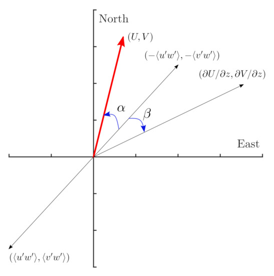
Figure 1.
Definition of and relative to the mean wind vector, the vertical gradient of the mean horizontal wind speed vector and the stress vector.
Consequently, is inherently assumed in numerical models when applying a flux–gradient relation to express the vertical transport of horizontal momentum. Berg et al. [7] observed vertical profiles of , which were non-zero, using measurements from a profiling lidar up to 200 m at Høvsøre, a close-to-flat site in Denmark. However, as mentioned by the authors, the observed misalignment could have been a product of the surface heterogeneity at the site.
In a study focused on low-level jets over open-water fetch, Svensson et al. [8] showed a mismatch between lidar-observed and WRF-derived momentum flux projected onto the direction of the mean wind, where lidar-based second-order statistics were filtered due to the effect of the probe volume when compared to sonic anemometer measurements. However, they did not address the limitations of the WRF model with regards to the flux–gradient relation validity.
Using large-eddy simulation (LES) of the neutral, unstable, and stable over flat terrain, Berg et al. [7] found values close to zero throughout the PBL. Kosović and Curry [9] performed an LES of the stable PBL and found a maximum of , but they did not attempt to further investigate the misalignment (personal communication).
This work presents mean wind and momentum flux vertical profiles computed both at an offshore and an onshore location using observations from a long-range profiling Doppler wind lidar and the WRF model output from the New European Wind Atlas (NEWA) project (hereafter NEWA-WRF), which uses a PBL scheme where the momentum transport is parameterized with a flux–gradient relation [10]. The objectives herein are threefold:
- The comparison of onshore and offshore vertical profiles of and between lidar observations and the NEWA-WRF output;
- Analysis of the behavior of as well as the wind direction bias between lidar observations and the NEWA-WRF output as a function of atmospheric stability;
- The evaluation of and profiles using idealized LESs under offshore- and onshore-like surface conditions.
In the preliminary study of Santos et al. [11], negative values of were observed by analyzing offshore lidar measurements. The present work extends the work in Santos et al. [11] by assessing the validity of the flux–gradient relation, i.e., whether or not approaches zero, using not only offshore, but also onshore, lidar measurements. Further, we include the analysis of the vertical profile of using idealized LES with surface boundary conditions resembling onshore and offshore conditions. We also discuss the consequences of the departure from flux-gradient relation for, e.g., mesoscale models.
2. Methodology
2.1. Site and Instrumentation
We present results from two measurement campaigns, one offshore and another onshore, where a long-range pulsed profiling Doppler lidar (WindCube WLS70 from Leosphere) was deployed next to meteorological masts for one-year measurement campaigns. Figure 2 shows the location of both sites: one at the FINO3 research platform (55°11.7′ N, 7°9.5′ E) and the other next to the Hamburg meteorological mast (53°31.2′ N, 10°6.31′ E).
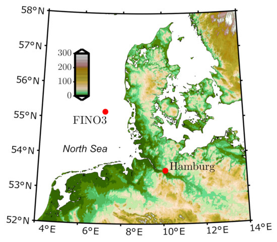
Figure 2.
Map of northern Europe with the location of the offshore (FINO3) and onshore (Hamburg) sites as red dots. The colorbar indicates the height in meters above sea level.
The WLS70 measured the radial or line-of-sight velocity at four azimuthal positions separated 90, namely . This conical scanning pattern is performed with an angle of from the vertical. Pulses were sent to the atmosphere at each azimuth for more than 2 s and the wind vector was derived every ≈10 s every 50 m from 100 up to 2000 m above the lidar level. The lidar probe volume length, defined by the full width at half of the expected maximum (FWHM) of the lidar’s along-beam sensitivity function, is ≈75 m [12]. Due to a persistent negative bias at 300 m, already noticed in previous work [11], this measurement level was removed from this analysis.
At FINO3, the lidar was placed at 24.5 m above mean sea level (amsl) and measured for a full year next to a 100-m tall meteorological mast, instrumented with cup anemometers at 30, 40, 50, 60, 70, 80 and 106 m. Hereafter, all heights are referred to amsl. Pena et al. [13] combined the first nine months of cup anemometers and lidar measurements to characterize the mean wind profile from 30 m up to 1000 m at the site.
At the onshore site, the lidar was measuring for a one-year campaign 170-m away from a 280-m high television tower located southeast of downtown Hamburg. The tower is instrumented with METEK USA-1 sonic anemometers from Metek GmbH, at 50, 110, 175 and 250 m. Brümmer et al. [14] showed a comprehensive introduction of the site and its wind climatology. Floors et al. [12] used these onshore lidar measurements, among others, to assess the influence of baroclinicity on the measured wind profile.
2.2. Data Selection and Filtering
The FINO3 dataset was selected based on the entire lidar measurement campaign, from September 2013 to October 2014. For the Hamburg site, we selected the first two months of measurements from 6 April 2011 to 2 June 2011 where the lidar was operating without breaks and properly aligned with the north.
For both sites, the data were filtered according to the carrier-to-noise ratio (CNR), which can be used as a quality measure of the estimation. Values with CNR higher than dB are considered valid in this work. Only wind profiles with valid data at all heights up to 500 m were selected. In addition to the CNR threshold, data were excluded when the radial velocity greatly exceeds the median value over a 30 min period, i.e., .
From the observations, we computed 30-min statistics throughout this work. From a sample of 10,926 30-min periods at FINO3, we applied the above filters to obtain 76.2% of valid data (8323) up to 500 m. At the Hamburg site, 2719 30-min periods were filtered so we obtained 40% of valid full profiles (1089).
At FINO3, high-frequency measurements from sonic anemometers were not available and so we could not directly compute the Obukhov length (L). Hence, we used the potential temperature difference as a proxy for atmospheric stability. The potential temperature difference is defined as , where is the potential temperature using concurrent air temperature measurements at 30 m and is the water temperature measurement at 6-m depth from a nearby buoy. The criterion for stability classification reads simply as K for unstable conditions and K for stable conditions.
At Hamburg, sonic anemometer measurements at 50 m represent surface-layer conditions [12]. Therefore, we computed L using these measurements and defined stability regimes as m representing neutral, 0 m m stable, and m m unstable conditions.
For FINO3, the wind direction reconstructed from the lidar and a wind vane at 100 had an offset of –11.7° [13]. Thus, we apply this offset in our computations. At Hamburg, the lidar was aligned with the north for the selected period, so no offset was applied.
2.3. Observed and Modeled Momentum Fluxes
Using observations from a profiling lidar, the momentum fluxes can be computed from the difference between the radial velocity variance of lidar beams from two opposing azimuthal measurements. This was originally proposed by Eberhard et al. [15] and more recently applied by Mann et al. [4],
where is the lidar offset mentioned above, defined by the angle between the laser beam and the north. For a detailed derivation, see Appendix B.
Here, we assume horizontal homogeneity of the wind field, as we combine radial wind speeds from a number of points which are separated by up to 261.8 m, at the 500-m height level. Therefore, we expect that the vertical profiles of momentum fluxes up to 500 are better estimated using Equation (5) at the offshore than at the onshore site given the possible contamination from surface inhomogeneities at the latter site.
We choose to evaluate the NEWA-WRF outputs in this work, which were described in detail by Hahmann et al. [10]. These outputs offer a time series of a number of meteorological variables covering the period of both lidar campaigns, with a temporal and horizontal resolution of 30 min and 3 km, respectively, and seven vertical levels at 50, 75, 100, 150, 200, 250, and 500 m. A linear interpolation over the spatial domain was performed using the nearest neighbor grid cells to extract the time series at FINO3 and Hamburg locations. Hahmann et al. [10] compared the mean wind speed and wind direction profiles using several PBL schemes in the WRF model against observations from several meteorological masts, including FINO3. A further comparison of the NEWA-WRF outputs using more meteorological masts was performed by Dörenkämper et al. [16]. The results of these comparisons demonstrated that a modified version of the Mellor–Yamada Nakanishi–Niino (MYNN) scheme [17] resulted in the lowest wind speed bias at most sites.
The MYNN level 2.5 (MYNN2) is a local scheme, i.e., is derived from local quantities. We can thus estimate the local momentum fluxes using Equations (1) and (2) from the NEWA-WRF output by computing first as
where l is a master length scale, with e being the turbulent kinetic energy (TKE), which in MYNN2 is based on the prognostic TKE from Mellor-Yamada [18], and S is a stability function. Since l is not stored in the NEWA-WRF output, we derive it following the work of Nakanishi and Niino [17].
2.4. Idealized WRF-LES
Previous LESs under neutral, stable, and neutral PBLs performed with a surface condition typical of an onshore site showed [7]. We therefore performed two idealized LESs of a neutral PBL over a flat surface; one over water, i.e., a roughness length of 0.0002 m, and the other over land, i.e., a roughness length of 0.65 m, which is the value found over the urban sector at the Hamburg tower [19]. The LESs were performed using the WRF model (version 4.1.2) with a single domain of m in the two horizontal and vertical directions, respectively, with a horizontal resolution of 15 m and a Coriolis parameter correspondent to the latitude of the FINO3 site and the Hamburg tower for the offshore and onshore simulations, respectively. The vertical grid spacing of ≈5 m was kept constant up to 250 m and stretched out thereafter. We used a time-step of 0.2 s and the subgrid-scale model of Deardorff [20].
The simulations were performed for a dry atmosphere. The initial potential temperature was kept constant (289.5 K) up to 700 m, where we imposed an inversion of 10 K km upwards. At all vertical levels, the initial u and v velocities were set to 11 and 0 m s, respectively, at FINO3 and to 10 and 0 m s, respectively, at Hamburg to try to match the highest observed values at both sites. MOST was applied at the surface via the WRF-in-built surface-layer scheme. The LES was run for 12 h, a heat flux of 0 K m was imposed at the surface, and periodic boundary conditions were applied.
The relevant parameters within the whole domain were output every 10 s within the period 10.5–11.5 h because we found the highest velocity for both simulations within this hour. The statistics were computed over this one-hour period (such as means, variances, and covariances) and then spatially averaged over the whole domain.
The total momentum fluxes were computed by adding the subgrid to the resolved parts. Note that the coordinate system, in this case, is relative to the wind direction at the PBL top.
3. Results
The FINO3 and Hamburg sites are only separated by 267 km, hence they are influenced by the same large-scale weather patterns. At both sites, westerly winds are prevalent [13,14]; therefore, we select wind direction sectors of and for FINO3 and Hamburg, respectively, using lidar measurements at 100 m as reference for the wind direction. At FINO3, this sector represents one with a several-hundred-kilometer fetch, whereas at Hamburg, this is the ‘urban’ sector, which is characterized by industrial buildings and warehouses [14]. The selected sectors represent ≈ of the amount of winds at FINO3 and ≈ for Hamburg. A sensitivity analysis on the size of the wind sector was performed (not shown) and we did not find a significant difference in the characteristics of vertical profiles of wind speed, wind direction and momentum fluxes.
Figure 3 and Figure 4 show the vertical profiles computed from the lidar measurements (full lines) and concurrent computation using the NEWA-WRF outputs (dashed lines) within the westerly sector of FINO3 and Hamburg, respectively. The shaded area represents the standard error of the mean given by , where is the standard deviation of each vertical level and N the number of valid profiles up to 500 m. The mean PBL height given by NEWA-WRF at FINO3 is 925 m and at Hamburg is 858 m.
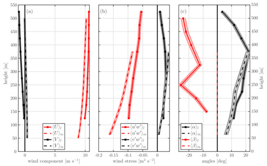
Figure 3.
Mean vertical profiles of (a) horizontal wind components, (b) momentum fluxes and (c) wind turning angles at FINO3. The full lines are lidar observations (l) and dashed lines represent the NEWA-WRF output (m). All profiles are within and are computed from 3343 30-min samples, where the shaded areas represent the standard errors of the mean.
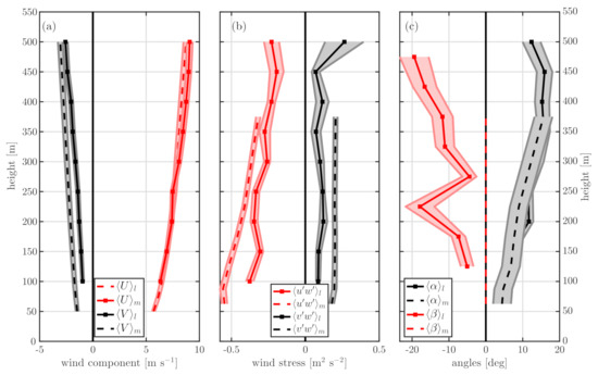
Figure 4.
Mean vertical profiles of (a) horizontal wind components, (b) momentum fluxes and (c) wind-turning angles at Hamburg. The full lines are lidar observations (l) and dashed lines represent the NEWA-WRF output (m). All profiles are within and are computed from 616 30-min samples, where the shaded areas represent the standard errors of the mean.
3.1. Bias on Wind Turning
When comparing the vertical profiles of horizontal wind components at FINO3 (Figure 3a), the NEWA-WRF wind veers (turns clockwise) with height in a lesser degree than what is observed. This underestimation of the turning of the wind is familiar in numerical weather models [3] and was previously observed using the instrument from this work [21]. The wind turning is also not properly simulated at the Hamburg site (Figure 4a); although the simulated zonal wind component of NEWA-WRF agrees well with the measurements, there is a difference in the vertical profiles of the meridional wind component. As previously mentioned, the lidar’s ability to measure all vertical levels at once makes it an ideal instrument to quantify such biases.
Figure 5 shows the vertical profiles of the wind direction bias between the lidar and NEWA-WRF for stable and unstable conditions at both sites. NEWA-WRF consistently underestimates the observed wind veer, with the highest bias under stable conditions, as expected [3]. The difference between onshore (Figure 5a) and offshore (Figure 5b) conditions is that, over water, the wind direction bias is small (≈) at 100 m and increases with height. Contrarily, over the urban fetch the bias is quite significant (>) at 100 m and decreases towards the PBL top, where it reaches similar values to those at offshore conditions. The wind turning bias behavior under stable conditions agrees with previous results over offshore conditions; Simpson et al. [22] argued that the PBL schemes generally enhance turbulence mixing under stable conditions, which results in an underestimation of both the wind shear and wind turning.
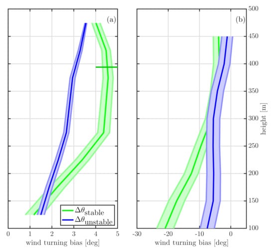
Figure 5.
Mean profiles of wind turning bias at FINO3 (a) and Hamburg (b), given by the difference between the lidar and NEWA-WRF wind directions (), under unstable (blue) and stable (green) conditions. The mean PBL height under stable conditions, based on NEWA-WRF, is plotted as a horizontal green line.
One possible reason for the wind direction bias at both sites is systematic mismatch between the simulated and actual stability condition. NEWA-WRF also outputs L, so we can compare the concurrent simulated and observed stability. At FINO3, unstable conditions represent 85.5%, based on the observed potential temperature gradient for all wind sectors. By comparing the stability measures of simulated and observed wind profiles, we find that stable conditions are correctly simulated 76% of the time, whereas 90% of the observed unstable profiles are also unstable based on the model output.
Under the urban sector at Hamburg, neutral conditions are predominant, as discussed by Gryning et al. [19]. For all stability conditions at Hamburg, the estimated PBL height from NEWA-WRF is above the measured profiles. When L computed by the sonic anemometer is compared to the output from NEWA-WRF, we find that 60% of the observed stable profiles are correctly simulated as such, whereas the number increases to 94% for the observed unstable profiles.
3.2. Momentum Fluxes and Lidar’s Turbulence Attenuation
For the analyzed westerly winds, both the observed and NEWA-WRF vertical profiles of momentum flux (Figure 3b and Figure 4b) show values close to zero and values decreasing in magnitude almost linearly with height. However, at both sites, there is an important mismatch between the lidar observations and NEWA-WRF for . This could be caused either by the computations involving Equation (6) or turbulence attenuation due to the lidar’s spatial averaging (or both).
For the analyzed period, the observed and NEWA-WRF vertical profiles of velocity gradients are rather similar (not shown). Therefore, if the bias comes mainly from the NEWA-WRF momentum fluxes, then our estimate of using Equation (6) could be flawed. However, we know that the lidar-derived momentum fluxes have an inherent bias due to spatial averaging along the lidar beam [4].
To gain insights into the origin of this bias, we estimate the lidar’s turbulence attenuation under neutral conditions using the turbulence spectral model of Mann [23] (hereafter, the Mann model), with a turbulent eddy-lifetime parameter , as recommended by the IEC standard [24]. describes the degree of anisotropy of turbulence; corresponds to fully isotropic turbulence. Figure 6 shows the ratio of the filtered to the unfiltered momentum flux as a function of the ratio of the lidar’s probe volume (i.e., the FWHM) to the turbulence length scale (). is another parameter of the Mann model.
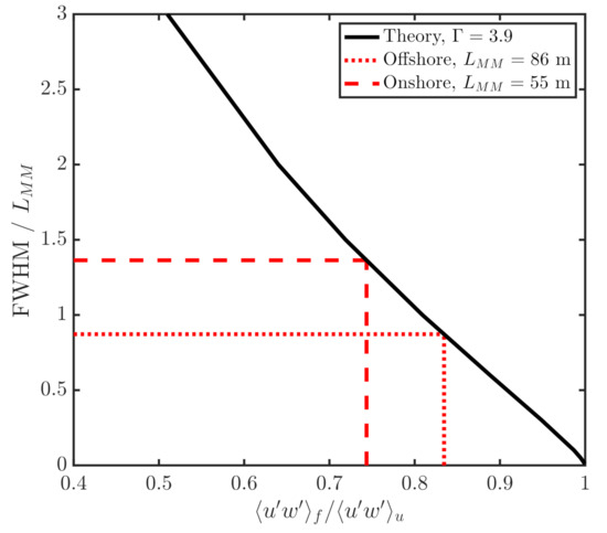
Figure 6.
Ratio of the filtered to unfiltered momentum flux as a function of the ratio of the lidar’s probe length to the turbulence length scale (). The dotted lines represent estimated values for onshore and offshore sites at 100 m.
The black full line in Figure 6 shows the prediction of the ratio using the Mann model. For a detailed description of the calculations, refer to Mann et al. [4]. For the WLS70 used in this study, m, so we only need to know the value of to compute the degree of filtering. We can estimate the turbulence length scale using the approximation by Kelly [25],
where is the standard deviation of the horizontal velocity and is the horizontal wind shear, which is computed here using the polynomial of suggested by Högström [26]. We account for the observations at all vertical levels of the masts. The length scale at 100 m is computed as a linear interpolation between the closest measurements at each mast.
The dashed lines in Figure 6 show that the turbulence length scale estimated at FINO3 is larger than that at Hamburg, which results in a larger attenuation of the momentum flux at Hamburg (74.4%) compared to that at FINO3 (83.4%). As turbulence length scales depend on atmospheric stability [27], we expect that the dominant unstable conditions at FINO3 result in larger turbulence length scales compared to those at Hamburg where neutral conditions are more often observed.
By compensating the lidar-observed values at 100 m with the results in Figure 6, we find a better agreement between the lidar- and NEWA-WRF derived values. However, its worth noticing that the NEWA-WRF momentum fluxes are parameterized from Equation (6) so the simulated momentum fluxes do not necessarily have the same magnitude as the observations. Furthermore, the attenuation estimated in Figure 6 is subject to uncertainties from the spectral turbulence model, the FWHM value, and the estimation (refer to Appendix A for the vertical profiles of estimated at each site).
3.3. The Angles of the Stress Vector with Mean Wind Vector () and with Mean Wind Shear Vector ()
Figure 3c and Figure 4c show the vertical profiles of and for offshore and onshore conditions, respectively. As expected from the LESs of Berg et al. [7], is close to zero near the surface and increases with height. Furthermore, the results using the NEWA-WRF output agree well with those of the lidar at both sites. However, note that a good agreement on could occur due to a combination of biases in both wind direction and momentum fluxes.
The most noticeable discrepancy between the lidar measurements and the NEWA-WRF output is on , since we use flux-gradient relation to derive the eddy fluxes with the NEWA-WRF output. This theory assumes this misalignment is zero. The misalignment for all heights is on average close to offshore and onshore. If we reduce the wind sector to , the mean for all heights is offshore and onshore, i.e., the result is not sensitive to the wind sector at either of the sites. Here, the non-linear behavior of with height, with a kink at 250 m, is attributed to faulty lidar measurements during both campaigns, as pointed out in Section 2.1.
The profiles and, hence, the validity of the flux–gradient relation are sensitive to the vertical gradients of the mean wind. Therefore, we expect that PBL schemes using the assumption of a flux–gradient relation (such as MYNN2 and other local PBL schemes) show a better performance when the vertical mean wind gradients are more significant, i.e., under stable conditions [28]. Figure 7 shows the vertical profiles of as a function of atmospheric stability for both sites. To avoid the spikes seen in Figure 3 and Figure 4, the value at the third measurement height is the result of a linear interpolation.
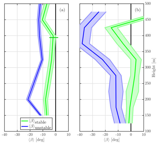
Figure 7.
Vertical profiles of for FINO3 (a) and Hamburg (b) under unstable (blue) and stable (green) conditions. The horizontal green line marks the PBL height under stable conditions based on NEWA-WRF.
The vertical profiles of , derived from the lidar observations, show that the misalignment can be as small as ≈ on average for offshore conditions and close to onshore, under stable conditions. Additionally, under stable conditions approaches zero close to the PBL top. Although fluctuating, the values under unstable conditions are always larger (in module) than those under stable conditions at both sites, as expected.
3.4. WRF-LES
Figure 8 shows the WRF-LES results with regard to the turning angles for a neutral PBL over a water-like and a land surface roughness. Over water and below 250 m (Figure 8a), is negative, partly due to the higher impact of the subgrid-scale model on the term compared to the term. Within the range of 250–550 m, is comparable to the observed values at FINO3. is nearly within a large portion of the PBL and increases (in magnitude) with height at the vertical level where both velocity gradients and eddy fluxes are near zero. Within the range 40–200 m, becomes slightly positive because of the combination of the impact of the subgrid-scale model on the eddy fluxes and the excessive vertical wind shear within the surface layer that the subgrid-scale model produces [29,30].
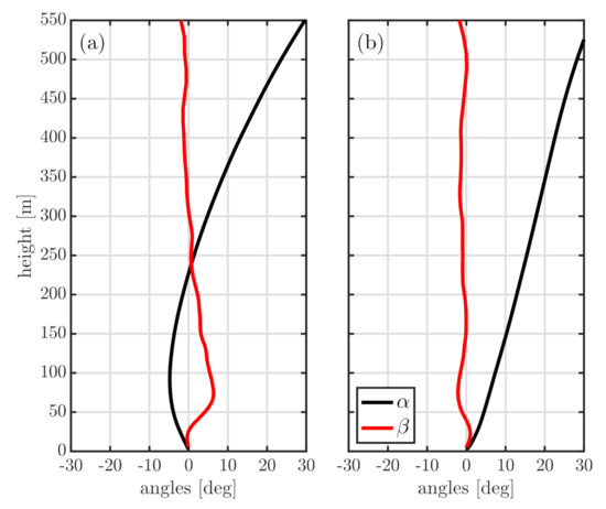
Figure 8.
Vertical profiles of turning angles computed from the idealized neutral WRF-LES over (a) water and (b) land.
Over land (Figure 8b), increases with height, is always positive, and is slightly higher than the observed values at the Hamburg tower. is, as in the offshore case, nearly within the first 550 m. Due to the high roughness of the onshore case, the resolved terms are less impacted by the subgrid-scale model and so does not show a strong departure from zero within the surface layer, although there is also excessive vertical wind shear.
4. Discussion and Conclusions
We extend the work from Santos et al. [11] and present novel lidar observations that show a clear misalignment between the vertical gradient of the mean wind vector and the stress vector, , up to 500 for both offshore and onshore conditions. The measurements were performed with a long-range Doppler wind lidar on the FINO3 offshore platform and close to the Hamburg weather mast. Such a misalignment is assumed to be zero by the PBL schemes that apply a flux–gradient relation and that are normally utilized within current numerical weather models and for wind resource assessment, e.g., the WRF model.
The observed -values increase from about at 100 m to about at 500 m at both offshore and onshore sites. During stably stratified conditions, where larger vertical wind gradients are present, is still negative but above and approaches zero at the PBL top. The value has a larger magnitude for unstable compared to stable conditions at all heights for both sites, and this magnitude increases with height onshore. Hence, the basic assumption of the flux–gradient relation, which we utilize to derive the eddy fluxes from the NEWA-WRF outputs holds better under stable compared to unstable atmospheric conditions, as expected, due to the larger coherent structures in the latter.
Our results show a bias between the vertical profiles derived from radial velocity measurements of a pulsed profiling lidar with those derived from the NEWA-WRF outputs. We assess the filtering effect inherent to the lidar’s probe volume averaging by combining the Mann model and estimations of the length scale for both sites. The angle between the stress vector relative to the mean wind vector (i.e., ) derived from the NEWA-WRF outputs agrees well with the lidar-derived values, both offshore and onshore. This agreement is likely caused by a balance between the wind direction and momentum fluxes’ biases.
We observe an underestimation of the wind-turning by the NEWA-WRF output at the offshore site and an opposite turning at the onshore site. We speculate that this is mainly due to a wrong surface roughness assignment (or wrong land-use description) at around Hamburg tower in NEWA-WRF. It is worth noting that the heterogeneous condition at the onshore site is far from the PBL scheme assumptions used to derive the flux–gradient relation. This challenge can be partly overcome by the use of three-dimensional PBL schemes [31].
The wind direction bias is larger (in magnitude) under stable atmospheric conditions for both sites. At the offshore site, the wind direction bias is small (≈) at 100 m and increases with height, whereas the bias decreases (in magnitude) with height at the onshore site. Sandu et al. [2] argued that such wind turning biases in mesoscale models are the product of artificial enhancement of the mixing by turbulence closures, which, in turn, modifies the Ekman pumping and has a direct impact on, e.g., the ability to simulate cloud formation mechanisms.
The idealized WRF-LESs, both onshore and offshore, also show values close to within the bulk of the PBL, further demonstrating first, the need to investigate the conditions at which this misalignment occurs and, second, the need to better represent the PBL with numerical models. Note that the simulations of Berg et al. [7] and Kosović and Curry [9] used a different LES framework than our WRF-LES. A real-time WRF-LES, like that performed by Schalkwijk et al. [32], might be useful for further investigating, e.g., whether or not forcing conditions affect the behavior of . Finally, an analysis of the impact of baroclinicity can also be performed with the lidar observations, since both barotropic and baroclinic conditions were included in the mean vertical profiles.
Author Contributions
Conceptualization, P.S. and J.M.; methodology, P.S., A.P. and J.M.; formal analysis, P.S., A.P. and J.M.; investigation, P.S.; data curation, P.S.; writing—original draft preparation, P.S.; writing—review and editing, P.S., A.P. and J.M.; visualization, P.S. All authors have read and agreed to the published version of the manuscript.
Funding
This work was partly funded by the Ministry of Foreign Affairs of Denmark and administered by the Danida Fellowship Centre through the “Multi-scale and Model-Chain Evaluation of Wind Atlases” (MEWA) project.
Data Availability Statement
The NEWA data are available from https://map.neweuropeanwindatlas.eu/ (last access: 20 March 2021). The FINO3 met mast and buoy data are available from https://www.bsh.de/ (accessed on 20 March 2021). The Hamburg weather mast data are available from https://wettermast.uni-hamburg.de/ (accessed on 20 March 2021). The LES and lidar data are available upon request.
Acknowledgments
We acknowledge the Test and Measurements section of DTU Wind Energy for the operation and maintenance of the lidar database.
Conflicts of Interest
The authors declare no conflict of interest.
Appendix A. Length Scale Estimation
Figure A1 shows the vertical profiles of the estimated length scale according to Equation (7) from observations at both sites. At the FINO3 site, where unstable conditions are predominant, the length scales decrease with increasing wind speed, partly due to the dominant neutral stability under high wind conditions. Contrarily, within the urban sector from the Hamburg tower, the length scale increases with increasing wind speeds, similarly to previous observations over flat and homogeneous land [33].
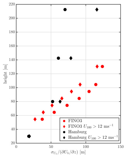
Figure A1.
The behavior with height of the ratio of the standard deviation of the wind to the vertical wind shear under onshore (black markers) and offshore (red markers) conditions within the selected wind sector. Circles represent median values of all data and diamonds are median values for wind speeds higher than 12 m s.
Appendix B. Derivation of Equation (5)
The lidar measures in the direction
where is the constant half-opening angle and is the variable azimuth angle. The line-of-sight velocity measured (positive away from the instrument) is where is the instantaneous wind vector at the position of measurement with, as mentioned in the main text, u is the East component of the velocity vector, v the North, and w the vertical. Usinq Equation (A1) the line-of-sight speed in the principle geographical directions (since is using the mathematical convention , , , and ) we get
Suppose that the turbulence at measurement height is statistically homogeneous in the horizontal directions, then the variance of the East and West beams can be written as
where a indicates the fluctuations around the mean. Subtracting these equations and using the trigonometric relation one gets
Similarly, using the North and South beams the equation for can be obtained. If the beams are not perfectly aligned with the principal geographical directions but deviates with an angle then the wind in the East–North coordinate system can be expressed as
References
- Skamarock, W.C.; Klemp, J.B.; Dudhia, J.; Gill, D.O.; Barker, D.M.; Duda, M.G.; Huang, X.Y.; Wang, W.; Powers, J.G. A Description of the Advanced Research WRF Version 3; Technical Report; NCAR/TN–475+STR, National Center for Atmospheric Research: Boulder, CO, USA, 2008. [Google Scholar]
- Sandu, I.; Beljaars, A.; Bechtold, P.; Mauritsen, T.; Balsamo, G. Why is it so difficult to represent stably stratified conditions in numerical weather prediction (NWP) models? J. Adv. Model. Earth Syst. 2013, 5, 117–133. [Google Scholar] [CrossRef]
- Brown, A.R.; Beljaars, A.C.M.; Hersbach, H.; Hollingsworth, A.; Miller, M.; Vasiljevic, D. Wind turning across the marine atmospheric boundary layer. Q. J. R. Meteorol. Soc. 2005, 131, 1233–1250. [Google Scholar] [CrossRef]
- Mann, J.; Peña, A.; Bingöl, F.; Wagner, R.; Courtney, M.S. Lidar Scanning of Momentum Flux in and above the Atmospheric Surface Layer. J. Atmos. Ocean. Technol. 2010, 27, 959–976. [Google Scholar] [CrossRef]
- Hasager, C.B.; Stein, D.; Courtney, M.; Peña, A.; Mikkelsen, T.; Stickland, M.; Oldroyd, A. Hub Height Ocean Winds over the North Sea Observed by the NORSEWInD Lidar Array: Measuring Techniques, Quality Control and Data Management. Remote Sens. 2013, 5, 4280–4303. [Google Scholar] [CrossRef]
- Sathe, A.; Mann, J. A review of turbulence measurements using ground-based wind lidars. Atmos. Meas. Tech. 2013, 6, 3147–3167. [Google Scholar] [CrossRef]
- Berg, J.; Mann, J.; Patton, E.G. Lidar-Observed Stress Vectors and Veer in the Atmospheric Boundary Layer. J. Atmos. Ocean. Technol. 2013, 30, 1961–1969. [Google Scholar] [CrossRef][Green Version]
- Svensson, N.; Arnqvist, J.; Bergström, H.; Rutgersson, A.; Sahlée, E. Measurements and Modelling of Offshore Wind Profiles in a Semi-Enclosed Sea. Atmosphere 2019, 10, 194. [Google Scholar] [CrossRef]
- Kosović, B.; Curry, J.A. A Large Eddy Simulation Study of a Quasi-Steady, Stably Stratified Atmospheric Boundary Layer. J. Atmos. Sci. 2000, 57, 1052–1068. [Google Scholar] [CrossRef]
- Hahmann, A.N.; Sīle, T.; Witha, B.; Davis, N.N.; Dörenkämper, M.; Ezber, Y.; García-Bustamante, E.; González-Rouco, J.F.; Navarro, J.; Olsen, B.T.; et al. The making of the New European Wind Atlas–Part 1: Model sensitivity. Geosci. Model Dev. 2020, 13, 5053–5078. [Google Scholar] [CrossRef]
- Santos, P.; Peña, A.; Mann, J. Flux-gradient relation and atmospheric wind profiles—An exploration using WRF and lidars. J. Phys. Conf. Ser. 2020, 1618, 032032. [Google Scholar] [CrossRef]
- Floors, R.; Vincent, C.L.; Gryning, S.; Peña, A.; Batchvarova, E. The Wind Profile in the Coastal Boundary Layer: Wind Lidar Measurements and Numerical Modelling. Bound. Layer Meteorol. 2013, 147, 469–491. [Google Scholar] [CrossRef]
- Peña, A.; Gryning, S.E.; Floors, R. Lidar observations of marine boundary-layer winds and heights: A preliminary study. Meteorol. Z. 2015, 24, 581–589. [Google Scholar] [CrossRef]
- Brümmer, B.; Lange, I.; Konow, H. Atmospheric boundary layer measurements at the 280 m high Hamburg weather mast 1995-2011: Mean annual and diurnal cycles. Meteorol. Z. 2012, 21, 319–335. [Google Scholar] [CrossRef]
- Eberhard, W.L.; Cupp, R.E.; Healy, K.R. Doppler Lidar Measurement of Profiles of Turbulence and Momentum Flux. J. Atmos. Ocean. Technol. 1989, 6, 809–819. [Google Scholar] [CrossRef]
- Dörenkämper, M.; Olsen, B.T.; Witha, B.; Hahmann, A.N.; Davis, N.N.; Barcons, J.; Ezber, Y.; García-Bustamante, E.; González-Rouco, J.F.; Navarro, J.; et al. The Making of the New European Wind Atlas—Part 2: Production and evaluation. Geosci. Model Dev. 2020, 13, 5079–5102. [Google Scholar] [CrossRef]
- Nakanishi, M.; Niino, H. Development of an Improved Turbulence Closure Model for the Atmospheric Boundary Layer. J. Meteorol. Soc. Jpn. Ser. II 2009, 87, 895–912. [Google Scholar] [CrossRef]
- Mellor, G.L.; Yamada, T. Development of a turbulence closure model for geophysical fluid problems. Rev. Geophys. 1982, 20, 851–875. [Google Scholar] [CrossRef]
- Gryning, S.E.; Batchvarova, E.; Brümmer, B.; Jørgensen, H.; Larsen, S. On the extension of the wind profile over homogeneous terrain beyond the surface boundary layer. Bound. Layer Meteorol. 2007, 124, 251–268. [Google Scholar] [CrossRef]
- Deardorff, J.W. Stratocumulus-capped mixed layers derived from a three-dimensional model. Bound. Layer Meteorol. 1980, 18, 495–527. [Google Scholar] [CrossRef]
- Peña, A.; Gryning, S.E.; Floors, R. The turning of the wind in the atmospheric boundary layer. J. Phys. Conf. Ser. 2014, 524, 012118. [Google Scholar] [CrossRef]
- Simpson, I.R.; Bacmeister, J.T.; Sandu, I.; Rodwell, M.J. Why Do Modeled and Observed Surface Wind Stress Climatologies Differ in the Trade Wind Regions? J. Clim. 2018, 31, 491–513. [Google Scholar] [CrossRef]
- Mann, J. The spatial structure of neutral atmospheric surface-layer turbulence. J. Fluid Mech. 1994, 273, 141–168. [Google Scholar] [CrossRef]
- IEC. IEC 61400-1. Wind Turbines–Design Requirements, 3rd ed.; International Electrotechnical Commission: Geneva, Switzerland, 2005. [Google Scholar]
- Kelly, M. From standard wind measurements to spectral characterization: Turbulence length scale and distribution. Wind Energy Sci. 2018, 3, 533–543. [Google Scholar] [CrossRef]
- Högström, U. Non-dimensional wind and temperature profiles in the atmospheric surface layer: A re-evaluation. Bound. Layer Meteorol. 1988, 42, 55–78. [Google Scholar] [CrossRef]
- Peña, A. Østerild: A natural laboratory for atmospheric turbulence. J. Renew. Sustain. Energy 2019, 11, 063302. [Google Scholar] [CrossRef]
- Shin, H.H.; Hong, S.Y. Intercomparison of Planetary Boundary-Layer Parametrizations in the WRF Model for a Single Day from CASES-99. Bound. Layer Meteorol. 2011, 139, 261–281. [Google Scholar] [CrossRef]
- Mirocha, J.D.; Churchfield, M.J.; Muñoz Esparza, D.; Rai, R.K.; Feng, Y.; Kosović, B.; Haupt, S.E.; Brown, B.; Ennis, B.L.; Draxl, C.; et al. Large-eddy simulation sensitivities to variations of configuration and forcing parameters in canonical boundary-layer flows for wind energy applications. Wind Energy Sci. 2018, 3, 589–613. [Google Scholar] [CrossRef]
- Peña, A.; Kosović, B.; Mirocha, J.D. Evaluation of idealized large-eddy simulations performed with the Weather Research and Forecasting model using turbulence measurements from a 250 m meteorological mast. Wind Energy Sci. 2021, 6, 645–661. [Google Scholar] [CrossRef]
- Kosović, B.; Munoz, P.J.; Juliano, T.W.; Martilli, A.; Eghdami, M.; Barros, A.P.; Haupt, S.E. Three-Dimensional Planetary Boundary Layer Parameterization for High-Resolution Mesoscale Simulations. J. Phys. Conf. Ser. 2020, 1452, 012080. [Google Scholar] [CrossRef]
- Schalkwijk, J.; Jonker, H.J.; Siebesma, A.P.; Van Meijgaard, E. Weather forecasting using GPU-based large-eddy simulations. Bull. Am. Meteorol. Soc. 2015, 96, 715–723. [Google Scholar] [CrossRef]
- Peña, A.; Gryning, S.E.; Mann, J. On the length-scale of the wind profile. Q. J. R. Meteorol. Soc. 2010, 136, 2119–2131. [Google Scholar] [CrossRef]
Publisher’s Note: MDPI stays neutral with regard to jurisdictional claims in published maps and institutional affiliations. |
© 2021 by the authors. Licensee MDPI, Basel, Switzerland. This article is an open access article distributed under the terms and conditions of the Creative Commons Attribution (CC BY) license (https://creativecommons.org/licenses/by/4.0/).