Abstract
Historically, the olive grove has been one of the most emblematic ecosystems in Mediterranean countries. Currently, in Andalusia, Spain, the land under olive grove cultivation exceeds 1.5 million hectares, approximately 17% of the regional surface. Its exploitation has traditionally been based on the use of the available land and heterogeneous plantations, with different species adapted to southern Mediterranean climatic conditions, and to the management of the traditional olive cultivation culture. The objective of this work is to characterize the mechanical behavior of the atmospheric surface boundary layer (SBL) (under neutral stability) interacting with different olive grove configurations. Experimental tests were carried out in the Boundary Layer Wind Tunnel (BLWT) of the Andalusian Institute for Earth System Research (IISTA), University of Granada. Three representative configurations of olive groves under neutral atmospheric conditions were tested. The wind flow time series were recorded at several distances and heights downwind the olive plantation models with a cross hot wire anemometry system. Herein, this paper shows the airflow streamwise, including the mean flow and the turbulent characteristics. The spatial variability of these two mechanical magnitudes depends on, among others, the size, the agro-forest length, the layout of the tree rows, the porosity, the tree height, the crown shape and the surface vegetation cover. The aerodynamic diameter and Reynolds number for each agro-forest management unit are proposed as representative variables of the system response, as these could be related to olive grove management. The plantation, in turn, conforms to a windbreak, which affects the microclimate and benefits the elements of the ecosystem. Detailed knowledge of these variables and the interaction between the ecosystem and the atmosphere is relevant to optimize the resources management, land use and sustainability of the overall crop. Thus, this paper presents preliminary work to relate atmospheric variables to environmental variables, some of which could be humidity, erosion, evapotranspiration or pollen dispersion.
1. Introduction
Historically, the olive grove has been one of the most emblematic ecosystems in Andalusia (south of Spain), where there are more than 1.5 million hectares of olive orchard land, representing 17% of the regional surface [1]. The livelihood of a high percentage of the population revolves around this ecosystem, emphasizing its relevance from social, environmental and economic-financial points of view. However, in the last years, climate change is producing uncertainty about crops sustainability in the Mediterranean areas, risking the production of the olive groves [2].
The traditional olive grove is characterized by an irregular pattern, resulting from the use of wild olive trees, creating heterogeneous plantations with different species adapted to the topography and characteristics of the soil. In such cases, olive trees usually exhibit high arboreal bearing and natural or cultivated vegetation cover for cattle farm purposes [3]. Currently, changes in land use and intensive olive growth based on hedge-shaped crops have changed plantation systems. The olive grove type, its cover and the silviculture treatments applied, regardless of the exchange processes, define the system dynamics and the interaction with the atmosphere [4].
The atmospheric surface boundary layer (SBL) encompasses the bottom 5% (first 50–100 m) of the atmospheric boundary layer (ABL), which is the lowest part of the atmosphere, where we live and where crops are grown [5]. The microclimate around the ecosystems varies depending on forest height and density, trees structure, ground cover, topography, among others [6]. The dynamic interaction between the SBL and the Earth’s surface, forests and agro-ecosystems includes the exchange processes and flows of energy, moisture and gases, and these are directly related to pollen concentration [7], gases and CO exchanges [8], pollutants dispersion [9], bushfires propagation [10], erosion and morphological processes [11], as well as the whole set of variables related to the mechanics of the system [12] and which are in a coupling with atmospheric processes [13].
The studies of Gardiner et al. [12] and Brunet [6] discuss and summarize the most recent works on the interaction between wind and trees, including the mean flow and turbulent characteristics in grassland [14] and in forested canopies [15]. However, these studies do not provide a direct comparison between different layout configurations and plant species composition—with its morphological characteristics—for the same type of ecosystem. Advances in the study of vegetation–wind interaction and the near weak flow behind trees [16] are analyzed through statistical models or using on-site measurements to figure out how changes in trees density affect the wind speed and the turbulence. Other studies are focused on the impact of landscape fragmentation [9], the role of wind-trees interaction under wind storm conditions [17] and the consequent tree damage processes according to the work of Albrecht et al. [18] and Kamimura et al. [19].
In situ measurements can be used to analyze the dynamic response of trees to wind loads and possible damages to vegetation [9,20] and, similarly, the influence of vegetation and trees structure on the flow in a particular location [21]. Field data allow vertical wind profiles and direct measurements to be obtained at specific points, but this entails a high degree of difficulty because of its high temporal and spatial variability [22]. This is why the need arises to carry out laboratory experiments and wind tunnel tests, in order to complement and obtain data on a greater level of detail and under controlled conditions. Most of these studies are focused on the analysis of flow behavior around and above artificial or natural vegetation models, including variations in spatial layout, trees structure, spacing and density [9,11,23,24], as well as the Reynolds number dependence regarding the forest canopy [22]. According to Cheng et al. [25], the plantation layout, number of rows and arrangement affect the downwind airflow recovery and play a key role in the protection against erosion [26]. In some cases, the results can be complemented with data from computational fluid dynamics analysis (CFD) [27] and other numerical simulations [28].
A plantation works as windbreaks, allowing air flow through it according to porosity, tree structure and spatial configuration, modifying and defining the streamwise flow, affecting nearby ecosystems [29]. According to this behavior and the above information, it is assumed that the development of an olive agro-forest substantially modifies the air flow kinematic variables and the turbulence properties. However, it also changes the spatial and temporal gradients of environmental variables and processes, such as erosion processes, surface moisture, air humidity flows, evapotranspiration and pollen and seed dispersion, among others. The objective of this work is to characterize the mechanical behavior of the SBL (under neutral stability) interacting with different olive grove configurations. For this purpose, the spatial evolution of the wind dynamics was calculated from temporal wind speed measurements, recorded in regularly spatially distributed points located behind the agro-forest system (in the x, y and z directions), based on the physical principles previously provided. Physical experiments were carried out in the BLWT of the University of Granada [30], based on a dimensional analysis of the variables of interest and the particularities of the Andalusian olive grove.
2. Physical Principles and Dimensional Analysis
This section contains the physical principles of ABL regarding its air flow and turbulence characteristic. Only mechanical turbulence, generated by friction between the wind field and the olive grove, have been considered. Three main elements has been taken into account for the olive grove: tree unit, tree row and plantation/agro-forest system. Hereafter, the methodology is described, including the dimensional analysis of the problem.
Wind flow velocity over the Earth’s surface is reduced due to the turbulent motions caused by the interaction with the topography, ecosystems, etc. In this dynamic interface, it is recommended to perform a dimensional analysis of variables involved in the processes of interest, which allows the system to be analyzed when there is limited knowledge of the system physics [31]. This analysis allows the experimental measurements of a specific setup to be extrapolated to a global system. Dimensionally homogeneous equations are sought to ensure dynamic similarity, reduce the number of variables and explain the mechanistic effects inside a given airflow [32].
When managing an olive plantation, the objective is to optimize resources, particularly water resources, and maximize production. Note that the layout depends on the management and exploitation of the agro-forest and synthesize the rich experience acquired by the Mediterranean countries in the last 3000 years. To this end, plantations are made with trees distributed in different patterns, usually in rows with corridors, that facilitate tillage and harvesting, with production-focused silvicultural treatments (traditional or intensive). The types of soil, topography, vegetation, etc. are translated into different functional relationships. For this reason, in this paper, several cases of typical functional relationships in the olive grove are analyzed.
The management problem was divided into a 2DV, i.e., analysis in the streamwise direction (Figure 1a) and a 2DH, i.e., analysis in the crosswise direction (Figure 1b). Figure 1 is a 2D scheme of the interaction between agro-forest and wind dynamics. We aim to evaluate the physical quantities that can be used to describe the transformation of wind dynamics leeward of the agro-forest, i.e., the instantaneous wind velocity at different distances from the forest edge.
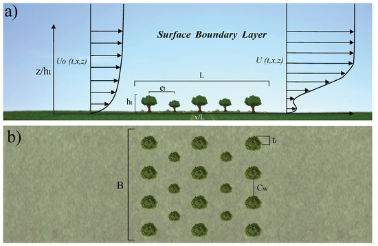
Figure 1.
Scheme of wind profile transformation in the SBL streamwise and crosswise an agro-forest system: (a) , side view; and (b) , top view. is the tree height, is the streamwise distance between trees, is the tree crown radius, is the crosswise corridor width, L is the overall plantation length and B is the plantation width.
2.1. Dimensional Analysis
First, a dimensional analysis of the problem is performed; a 2D olive ecosystem is analyzed, assuming infinite width and no lateral variation. The first step of the dimensional analysis is to identify a complete set of independent quantities that determine the value of the wind speed over and behind the forest. For each height z, the set of independent variables, related to wind velocity behind the agro-forest, are summarized as follows:
- 1.
- Physical properties: Air density , air dynamic viscosity and gravitational acceleration g.
- 2.
- Layout of the agro-forest (see Figure 1), including:
- Tree properties: Tree height and tree crown radius .
- Trees row properties: The streamwise distance between trees and the crosswise corridor width .
- Plantation properties: Overall length L.
- 3.
- Input: Instantaneous wind velocity profile upwind the forest, , used as reference velocity in this work, and friction velocity, , related to each other through the Von Karman expression, considering neutral atmosphere:where is the Von Karman constant and is the aerodynamic roughness length. In general, is assumed to be constant. However, for vegetation cover with discontinuities, this variable is markedly dynamic due to the natural flexibility of plants and its dependence on wind velocity and friction velocity [33]. In addition, this parameter affects the flow and modifies the vegetation itself and its surface characteristics. Performing a more formal analysis, would be selected as a variable for the dimensional analysis; however, since it is directly related to , for this specific case, is selected as input variable.
- 4.
- Output: Measured instantaneous wind velocity time series downwind the agro-forest, .
On the other hand, by carrying out the experiment during a period of time long enough to record a statistically representative time series, but short enough to assume that the experiment is a stationary process, the input and output wind velocities can be split into two components,
where is the time average wind velocity, is the time wind velocity fluctuation and the subindices o and l indicate input and output, respectively. Assuming stationarity of the process, the time variable is simplified.
A complete set of independent quantities is selected, which determine the time average wind speed value at any location behind the forest,
which comprises a total of independent variables. It is convenient to separate the variables that hold for all the experiments to build a subset of independent quantities, Subset 1 with and .
Choosing a base Subset 1, of independent quantities, , then , three dimensionless monomial are obtained:
The remaining set of independent variables is a base Subset 2 of : , then . Using the base Subset 2, the base Subset 1 and the output variable, the following non-dimensional quantities are obtained:
where is the kinematic viscosity of the air, and the dimensionless quantities are: (I) streamwise row length; (II) tree crown length; (III) crosswise corridor width; (IV) plantation roughness length; (V) relationship between viscosity and friction due to plantation height; and (VI) relationship between plantation length and downwind system response. This last term (VI) approximates a Froude number, which relates inertial forces to gravitational forces. This allows relating the agro-forest length to the air flow characteristics streamwise.
2.2. Derived Quantities
The analysis and results depend on the spatial position in which they are performed, being their coordinates:
In this case, the height z is made dimensionless with the tree height . However, the vertical velocity profile is dependent on the ratio . From measurements at each location, subtracting the measured instantaneous wind velocity and its time average over a given period, the wind speed fluctuation, or gust components, , can be calculated. Theoretically, it is a Gaussian distributed variable with zero mean and non-zero variance. Thus, based on previous dimensional analysis, the dimensionless variance downwind of the agro-forest can be determined.
The variance should be considered as a first kind derived quantity. The local turbulence intensity and the local turbulence kinetic energy per unit mass downwind of the agro-forest are defined in terms of the local variances (horizontal and vertical). Thus, those quantities can be considered as second kind derived quantities, and their dimensionless forms are shown as:
- 1.
- First kind derived quantities:
- 2.
- Second kind derived quantities:
Furthermore, the velocity skewness , which complement the statistics of turbulence and represent the vertical transport of by the turbulence [34], is defined dimensionless as:
2.3. Approach to a 3D Analysis, Aerodynamic Variables and Regimes
In this work, the experiments are carried inside a wind tunnel. All the elements have dimensions quantifiable and correlated to the behavior of the system through the aerodynamic diameter and the Reynolds number.
With the help of dimensional analysis, the following second-order quantities, which define the agro-forest, can be calculated. The agro-forest layout can be described in terms of aerodynamic diameters of: (i) the tree row, ; (ii) of the tree unit, ; (iii) of the plantation, ; and (iv) the aerodynamic diameter of the tunnel , defined as follows:
where a and b are the height and width of the tunnel section, respectively, B is the plantation width, and is the aerodynamic row radius.
The layout of the olive grove and the air flow along the tunnel allows the assumption that the experimental setup is repeated transversely. Thus, tests can be performed in 2D, being generated small cross-sectional variations between the tunnel walls. Consequently, the experiment is controlled by four Reynolds numbers, defined by aerodynamic variables: (i) for the empty wind tunnel, ; (ii) for the tree unit, ; (iii) for each trees row, ; and (iv) for the plantation, , defined as:
From the variables above, the behavior of the plantation as a whole is defined. Responding to current exploitation techniques using aerodynamic variables. Thus, it must be determined whether the Reynolds number is high enough to ensure that the flow is full turbulent and the viscosity effects at the local scale are minimal.
3. Experimental Setup
Physical tests were carried out in the BLWT of the Environmental Fluid Dynamics Laboratory of the Andalusian Institute for Earth System Research (University of Granada). In this open-circuit wind tunnel (NPL Type), air flows straight in one direction and recirculates outside the tunnel. The tunnel has a total length of 22 m and a test section of 2.15 m × 1.80 m with a length of 15 m, constant in the streamwise direction (Figure 2).
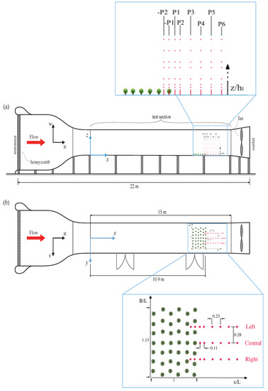
Figure 2.
Sketch of the BLWT: (a) elevation view; and (b) floor view, where profiles measured and scaled models position are shown. The blue squared enlargements show the olive tree model layout configuration, 22 measured profiles and 12 points for each vertical profile with relative distances represented as a function of , and . The red arrow shows the wind flow direction.
Experimental work in a wind tunnel involves to satisfy the kinematic and dynamic similarity principle. The wind velocity at any point in the model must be proportional to the prototype scale velocity, and all forces must be scaled with a constant scale factor. A geometric scale E is obtained according to the SBL height and the olive tree height to represent the agro-forest properly inside the wind tunnel, and the total area occupied by the forest is less than the total wind tunnel width. Thus, a working scale of E = 1:50 is defined to simulate an olive agro-forest surrounded by pasture with light vegetation cover. Moreover, the Reynolds number must be high enough and similar to the Reynolds number in the olive agro-forest. The aerodynamic diameters and Reynolds numbers for the input velocity and the agro-forest layout, obtained according to the analysis described in the previous section, are summarized in Table 1 and Table 2.

Table 1.
Aerodynamic diameters.

Table 2.
Reynolds numbers calculated for baseline conditions and m/s.
Olive trees have complex structures; thus, rigid scale models are used to accurately reproduce the trunk shape and irregularities of the crown. There are two types of models, i.e., Type 1 ( m and m) and Type 2 ( m and m), which simulate medium-sized olive trees typical of agro-forest systems. To simulate intensive olive grove exploitations, models of equal sizes are used. In this work, and according to the aerodynamic porosity defined by Manickathan et al. [35], a constant tree porosity value of approximately is assumed.
For traditional olive groves, models of both sizes are interleaved to reliably reproduce the controlled arrangement of olive trees. Six representative spatial configurations were designed in a spatial layout agro-forest with a length ( m, a width m and a tree separation distance of m (Table 3). In this study, three configurations were analyzed (see Figure 3), whose characteristics are summarized in Table 3.

Table 3.
Characteristics of three configurations tested in the wind tunnel, including the number of configuration C, the layout type (Grid (G) or Staggered (S)), vegetation cover, tree height (), streamwise distance between trees and tree crown radius ().
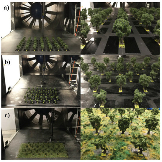
Figure 3.
Images of models tested: (a) grid olive grove configuration (intensive olive grove, C1); (b) staggered olive grove configuration (traditional olive grove without vegetation cover, C2); and (c) staggered olive grove configuration with cover (traditional olive grove with vegetation cover, C3).
Measurements were taken in 22 vertical profiles in the center and lateral sections, as shown in Figure 2. Data were recorded at 12 points in height per profile, and they were closer to each other in the area near the models, i.e., along the first m in the vertical direction, and progressively increasing the distance between points because the olive grove influence over the flow is predicted to be smaller as we move away from the surface.
For data acquisition (both flow calibration and olive grove tests), a constant temperature anemometer, namely a cross-wire X-probe, controlled by the system IFA 300® by TSI Inc. (Shoreview, MN, USA), was used to obtain measurements of the streamwise and vertical components of wind velocity () (Figure 4b). The probe was held by a TSI Standard Probe and placed on a 3D positioning system (Figure 4a), allowing accurate positioning of the hot wire sensor at measuring points.
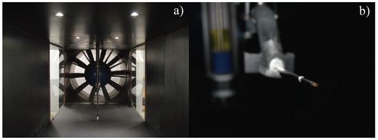
Figure 4.
Instruments and devices: (a) 3D positioning system of instruments inside the BLWT; and (b) cross hot wire anemometry system.
Data acquisition and processing were conducted using the software ThermalPro®, and a statistical analysis of the variables was subsequently performed with the same software. To ensure the data collected were representative, the sampling frequency for each point was 1 kHz for 131 s, under ergodicity assumption.
4. Results
In this section, from the experimental measurements, the first kind and second kind derived quantities are obtained, according to expressions developed in Section 2. As a velocity scale, we adopted a constant reference velocity (3 m/s). The results were expected to be similar for different wind velocities, as shown by Cheng et al. [25].
The results are presented as dimensionless variables for the mean wind speed , the turbulence intensity , the turbulent kinetic energy , the vertical velocity skewness , the aerodynamic surface roughness length and the friction velocity . As a reference length for measurements in the vertical direction, the height of the highest olive tree model (0.09 m) is used, designated . The distance between measuring sections is , and it changes between profiles in the streamwise direction (Figure 2).
4.1. Neutral Mean Flow Characteristics
As a preliminary step, the incoming flow homogeneity in the wind tunnel with an empty test section was performed for different velocities and elements for turbulence control [30]. Vertical profiles of the wind velocity (), turbulence ( and ), aerodynamic roughness length (), friction velocity () and Reynolds number () were obtained (Table 4) and taken as reference values for the ABL. These results were used for comparison with later tests on scale-models of olive groves.

Table 4.
Input values (ABL) obtained from wind tunnel flow calibration, where , m and m.
As Figure 5 shows, the flow in the test section is uniform in the streamwise and crosswise sections, with a wind velocity decrease of 30% and an increase of 13% in the turbulence intensity due to the wind profile generated by the wind tunnel floor roughness [36]. The vertical profiles were measured for the same section, as shown in Figure 2a, for later comparison with measurements downwind of the olive tree models. Only Profiles P1 and P4 are shown in Figure 5.
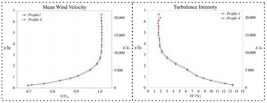
Figure 5.
Profiles measured for the empty wind tunnel, corresponding to Profile 1 (P1) and Profile 4 (P4) in Figure 2a. Vertical dimensionless wind velocity profiles (left); and turbulence intensity (right) measured on the wind tunnel central axis with an empty section. In both cases, the dimensionless values in height are shown as a function of tree height () and aerodynamic roughness height .
4.2. Mean Flow and Turbulence Around Olive Groves
For the three configurations tested, vertical profiles are compared along the main axis, corresponding to the central trees line, and vertical profiles on right and left sections include measurements between models. Two profiles are registered inside the olive grove from the coordinate origin, where the olive grove ends and the leeward side starts (-P1 and -P2 in Figure 2a). The models were distributed uniformly, thus it was proven that measurements in the central section are representative of the wind velocity distribution along the crosswise section.
Nine significant points were selected within the measured area, corresponding with Profiles P1, P4 and P6, in order to make a comparison of the results for each configurations analyzed. Figure 6 shows the position of these points in which measurements have been taken (coordinates z and x), according to the spatial distribution shown in Figure 2.
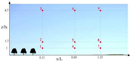
Comparisons have been made between each configuration and the results obtained previously for the incoming flow (ABL) (Figure 5). For this purpose, the values of the dimensionless wind speed, turbulence intensity and dimensionless TKE are shown. Some variation rates represented in percentages of variation were calculated, defined as:
Table 5, Table 6 and Table 7 show the dimensionless mean velocity difference , the dimensionless turbulence intensity and dimensionless turbulent kinematic energy at the test section for the reference ABL (empty section) and the same variables for the three olive grove configurations (C1–C3). In all cases, the mean velocity () is lower in the presence of olive trees (for this reason, the rate shows a negative value), while the turbulence parameters ( and ) are higher.

Table 5.
Mean values obtained for the grid configuration (C1) compared to the values obtained for the measured reference boundary layer. They are compared through ratios, represented as a percentage of the value of the reference conditions. The points of comparison are shown in Figure 6.

Table 6.
Mean values obtained for the staggered configuration (C2) compared to the values obtained for the measured reference boundary layer. They are compared through ratios, represented as a percentage of the value of the reference conditions. The points of comparison are shown in Figure 6.

Table 7.
Mean values obtained for the staggered with vegetation cover configuration (C3) compared to the values obtained for the measured reference boundary layer. They are compared through ratios, represented as a percentage of the value of the reference conditions. The points of comparison are shown in Figure 6.
Without an agro-forest system, the wind speed profile has a logarithmic shape (Figure 5). With an agro-forest system, the mean wind speed decreases between and at Points 1 and 7 (P1 and P6 at the bottom), and around at (Points 3, 6 and 9), where the effect produced by the ecosystem is very weak (Figure 7 and Figure 8). The comparison values show that the traditional olive grove without cover (C2) is the configuration that most influences the mean flow in the area next to the models. Regarding for the staggered configuration (C2), the percentages differ between 527% to 157% at the bottom and 1.90% to 0.72% at the top, for P1 and P6. However, the turbulent characteristics are maintained with a higher value for the case of the configuration with vegetation cover (C3), in both height and streamwise (Table 7).

Figure 7.
Mean wind velocity for the three configurations, measured leeward. In the abscissa, the distance is in the streamwise direction of wind flow normalized with respect to and in the ordinate is normalized with respect to . A greater velocity decrease is observed for the traditional olive grove (pink lines) when compared with the intensive olive grove (blue lines).

Figure 8.
Turbulence intensity profiles for the three configurations, measured leeward. In the abscissa, the distance is in the streamwise direction of wind flow normalized with respect to and in the ordinate is normalized with respect to . The turbulence intensity decreases as the distance from the olive grove increases, especially for the intensive olive grove.
Olive agro-forest presence is noticed up to an approximate height of , where the vertical profile is not logarithmic. The logarithmic shape is not recovered until a distance ; however, a trend is still visible. At tree height, for the traditional configuration C2, the velocity is almost zero in Profile 1 and, from Profile 2, this velocity increases in the streamwise direction (Figure 7 and Figure 8). Obstacle transmission is noticed from Profile 5, and it extends beyond a distance of .
In a comparison of the traditional configurations with and without vegetation cover (C2 and C3), the profiles have a more uniform shape in the presence of vegetation cover, not only for the mean velocity but also for the turbulence intensity (Figure 7 and Figure 8). However, is similar for a vertical distance of , and, at a height of , the flow is uniform, with a higher value for the case with vegetation cover.
In the following figures, the agro-forest length L is used as a reference length in the streamwise direction. In Figure 9 the color gradient covers the range of , with the lowest value corresponding to blue and the highest value to red. The intermediate values correspond to orange, yellow and green shades. In the case of turbulence intensity (Figure 10 and Figure 11b), the red range corresponds to the lowest values and the blue range to the highest turbulence levels, ranging . In Figure 12, the color scale ranges from white and light yellow for lower values to dark red for higher values, with a range of values of .
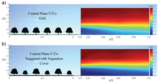
Figure 9.
Dimensionless mean wind velocity for the intensive olive grove C1 and the traditional olive grove C3 measured along the central axis downwind: (a) streamwise distribution of for the intensive olive grove; and (b) streamwise distribution of for the traditional olive grove with vegetation cover.
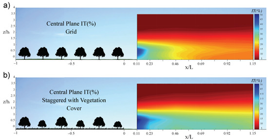
Figure 10.
Dimensionless turbulence intensity for the intensive olive grove C1 and the traditional olive grove C3 measured along the central axis downwind: (a) streamwise distribution of for the intensive olive grove; and (b) streamwise distribution of for the traditional olive grove with vegetation cover.
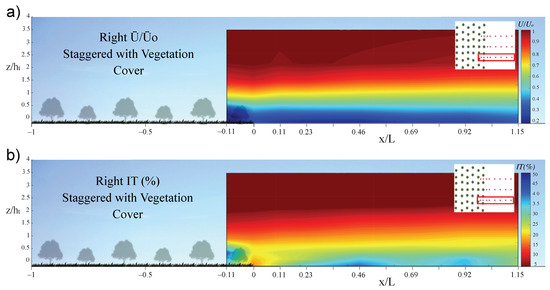
Figure 11.
Lateral profile measurements for the traditional olive grove with vegetation cover C3. Measurements taken between the olive tree models and behind them reveal: (a) the distribution of ; and (b) the streamwise distribution of .
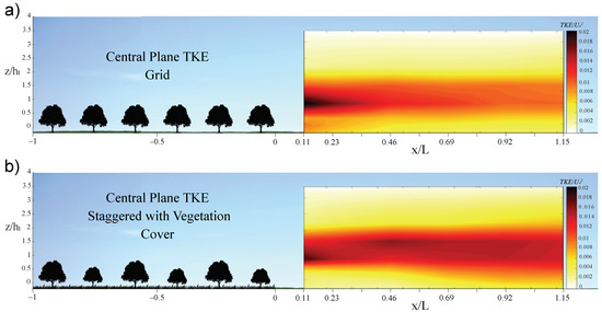
Figure 12.
Streamwise distribution of the dimensionless for: (a) the intensive olive grove without cover C1; and (b) the traditional olive grove with vegetation cover C3.
In Figure 9 and Figure 10, the results for intensive farming without cover (C1) are compared with those for traditional farming with vegetation cover (C3). Darker blue color indicate a greater distortion with respect to the reference values. For a height of , the wind velocities are more uniform, up to higher in the first case in areas close to the surface and lower in terms of turbulence intensity. For a distance of , the effects of intensive olive grove decrease; in contrast, these remains constant for the traditional configuration.
There are small differences between the lateral profiles and central profiles (Figure 11), due to some differences between the areas in which measurements were taken. A higher turbulence intensity is noticed for central section measurements at a distance of with respect to measurements for right section.
For the TKE, from a height of , the energy dissipation decreases and stabilizes vertically (Figure 12). The turbulence, generated at the surface, in the case of the traditional olive grove is developed earlier than in other configurations. As Figure 12 shows, there is an increase and spatial dispersion of the TKE along the flow downwind. In a comparison of the TKE values with and without the models (Figure 12), the flow around the olive groves has turbulence values of 300–600% higher than the free flow at a height of . By contrast, the TKE remains constant along the streamwise distance, most noticeable effect in the case of staggered olive grove.
In Figure 12, for intensive exploitation, a higher TKE is observed near the models up to a relative height of . The TKE increases and remains at high level from that point and along the flow direction for the traditional olive grove, reaching a value of almost double that of the intensive olive grove.
Vertical velocity skewness was analyzed, and the results for grid and staggered with vegetation cover configurations are shown in Figure 13. These results are in agreement with those obtained by Segalini et al. [24]. shows significant height (z) dependence and its behavior can be divided in three areas: (i) an area below the reference height (tree height ), in which the vertical skewness values are negative, so is not transported vertically; (ii) a second area from the height to about , in which the values are positive, and a vertical transport of is expected; and (iii) a third area that covers from to the end of the measurements taken, in which the values become negative again, although in the highest zone () a similar trend to that observed in the lower part is seen, towards values close to zero.
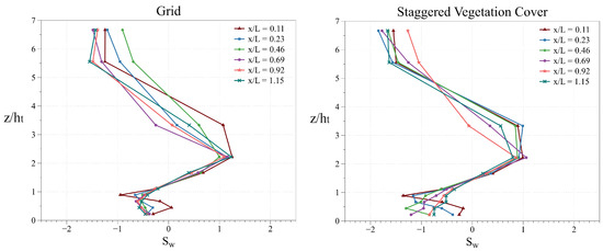
Figure 13.
Dimensionless vertical velocity skewness for grid and staggered with vegetation cover configuration.
These values are intimately related to turbulent kinetic energy, so a logical behavior can be observed if we compare them. The results obtained are consistent with those shown in the work of Hogan et al. [34], focused on the study of air flow over different types of canopy and spatial distributions.
5. Discussion
Andalusian olive groves are not only located in flatlands, but also in hills, terraces and near the mountain tops. Depending on their location and configuration, the impact on the landscape, hydrology and erosion and the amount of pollen in suspension that can later reach the populations will become more important.
First, a dimensional analysis of the variables involved in the problem was carried out, from which it is possible to infer the direct relationship between the kinematic and environmental variables and the physical characteristics of the ecosystem. The main physical characteristics are the height and tree crown radius of the tree ( and ), the streamwise distance between trees (), the crosswise corridor width () and the distribution of the plantation as a whole (B and L). From the dimensions and quantities detailed in this work, the Canopy Cover Fraction (), which estimates the tree cover of an agroforestry stand, could be determined, which is common in studies of ecology and agroforestry management.
According to Longo [37], defining the Jensen number as (where is the surface boundary layer thickness, which in this case is considered the wind tunnel total height, and is the roughness height, which in this case corresponds to the tree height ). Assuming the constant value in the model and the prototype, we define the geometrical scale. To ensure that the scale ratio of the roughness height is the same that the scale ratio of the boundary layer, where , being , equal to 4.5 m/0.09 m = 90 m/1.8 m, a scale of E = 1:50 was selected.
Because this experimental work employs rigid models, a small deviation in the turbulence values is expected. In general, it is recommended to limit the use of dynamic models due to, among others, the difficulty of reproducing the Reynolds number [38]. Based on the results of the measurements taken inside the agro-forest (Figure 11), the porosity of the plantation, due to the spacing between trees and the area around the trunks, allows the air flow, thus avoiding the reverse flow behind the ecosystem.
Neutral atmospheric stability was used, due to the limitations of mechanical wind tunnel testing [30]. However, according to the results of Moon et al. [13], there is a small contribution from changes in atmospheric stability, so the main change is generated by the wind speed.
For each spatial position, the global measurements defining the turbulent characteristics of system are the turbulence intensity , Turbulent Kinetic Energy (), vertical velocity skewness and shear velocity . Furthermore, the Reynolds number (), which describes the degree of turbulence related to the viscous forces, is estimated for the empty wind tunnel, the tree unit, the tree row and the plantation (, , and , respectively). As obtained for the initial flow conditions with the empty wind tunnel, the reference Reynolds number () is sufficiently high to neglect the influence of viscous forces. If we compare it with , and , as shown in Figure 14a,b, the values are much lower, due to the influence and closeness of the models, increasing as we move away from these and the flow returns to its initial state. The value of is generally higher for the grid layout configuration, especially in the case of , due to the absence of obstacles, since in the staggered configuration there are trees between the rows (Figure 3). However, the value of for the plantation is high enough to be considered independent of the obstacle, in this case, the ecosystem.
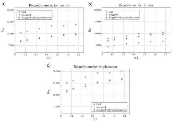
Figure 14.
Reynolds number calculated for each profile position: (a) Reynolds for tree row ; (b) Reynolds for tree (right); and (c) Reynolds for plantation .
The experiments of this study were carried out for flat terrain assuming that the experimental setup is repeated transversely and the tests are performed in 2D. Taking as reference the staggered configuration with vegetation cover, three profiles were selected for comparison (right, central and left), corresponding to Profiles 2, 4 and 6 (P2, P4, P6, in Figure 2). Comparing how the results differ slightly from each other, the hypothesis that, for the crosswise-section, the difference between the profiles is not relevant and the 2D results provide representative data of the plantation could be assumed. The system is ergodic although the Reynolds number criteria are not fully met in the near field profiles. However, it is fulfilled in the medium field and far field profiles. Therefore, the ergodicity is confirmed in the tests performed, and it is assumed that the ensemble average coincides with the time average (stationary system). As shown in Figure 15, the variation in the profiles measured for the central, right and left sections is small; in this way, the analysis performed and the results obtained could be extrapolated to the plantation as a whole.
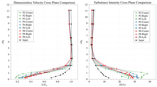
Figure 15.
Comparison of dimensionless mean wind velocity profiles (left) and dimensionless turbulence intensity profiles (right), obtained in Profiles P2, P4 and P6 and sections right, central and left (Figure 2), for the staggered with vegetation cover configuration. The black dotted line represents the profiles obtained upwind the olive configuration.
According to the results shown in Figure 16, the airflow recovery occurs progressively, being recovered in its practical totality at a height of , that is, twice the height of the tree. The profiles measured inside the plantation (-P2) show a greater reduction in velocity and increase in turbulence, due to its location as well as the existence of surface vegetation. However, in Position -P1, an acceleration of the flow and a decrease in turbulence can be observed. This acceleration phenomenon is related to the shape of the trees and the trunk height, but also it is associated with the porosity at that point.
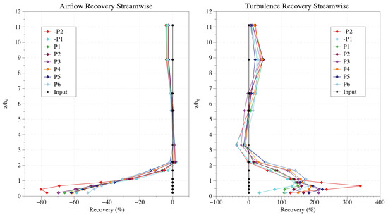
Figure 16.
Comparison of the streamwise recovery dimensionless mean wind velocity profiles (left) and dimensionless turbulence intensity profiles (right), obtained in the central section (Figure 2), for the staggered with vegetation cover configuration. This variation was calculated according to Equations (10)–(12), and part of its values are shown in Table 7.
The recovery effect shown in Figure 16 demonstrates the function of the olive grove as a windbreak. On the other hand, Figure 7 and Figure 8 show the differences between the studied configurations due to the plantation porosity and its spatial distribution, which is in agreement with the works of Podhrázská et al. [39] and Pan et al. [40].
Maintenance and management of current and new olive grove allotments have become a challenge for managers and decision makers because of the new intensive farming models that have appeared in the last decade. Decreases in precipitation and temperature in Mediterranean regions are expected to diminish production and make the sustainability of olive groves difficult [41,42]. In light of the results obtained, it is considered necessary to carry out surveys of the land topography, trees structure and density, vegetation cover, surface flow and atmospheric conditions, to optimize and manage the ecosystem in a sustainable and efficient way.
Some variables analyzed in this work are involved in the dynamics of ecosystems and should be incorporated into a management model, taking into account their direct relation to environmental variables such as pollen concentration, erosion processes or water availability, among others [7,10,42,43]. The olive grove influences the micrometeorology and is involved in the interaction between the surface and atmosphere, thus turbulence parameters are fundamental in the surface transport of heat, humidity and momentum.
6. Conclusions
The aim of this work is to analyze the interaction of different olive agro-forests, representative of Andalusia exploitations, with the air flow dynamics in the atmospheric surface boundary layer (SBL). This interaction was studied through wind tunnel tests to obtain a comprehensive understanding of exchanges and variations in the mechanics of the system, as well as to quantify kinematic variables that define the SBL, whose spatial and temporal gradients have significant effects on many environmental processes. These processes include soil erosion, evapotranspiration and water vapor fluxes and seeds and pollen dispersal distance, among others.
These kinematic variables, for neutral atmosphere conditions, were measured in three different sections, inside and behind the forest. Measurements include 22 vertical profiles for each configuration for a streamwise distance longer than the total length of the plantation.
Three olive grove configurations were modeled with a scale factor of E = 1:50, according to the Jensen number, as explained above. Every configuration is representative of Andalusian olive groves and had different layouts, trees composition and vegetation covers. The extension of the interaction of the olive agro-forest and the wind dynamics depends on the overall length (L) and width (B) of the forest, the streamwise distance between trees (), the crosswise corridor width (), the tree height (), the tree crown radius (), the characteristics of the soil cover, the incoming wind profile and the turbulence characteristics.
Windbreaks or plantation arrangements play a fundamental role in the ecosystem processes. They reduce velocity, modify the turbulence and affect the microclimate, but, at the same time, it is essential to ensure the airflow through the agro-ecosystem, which depends on the spatial arrangement and characteristics of individual trees. This is in agreement with the results of several studies, such as the one presented by Podhrázská et al. [39] and Pan et al. [40].
In this work, sustainability and traditional culture of the olive grove are combined with aerodynamic variables. The aerodynamic diameter of each agro-forest management unit studied is proposed as a representative variable of the system response and is directly related to the management and silvicultural treatment of the olive grove.
The results and conclusions obtained are applicable to the specific tree crown and trunk tested, so that, for other tree types, structures and spatial configurations, the results will change. The following conclusions can be derived from this study:
- 1.
- Regarding to wind velocity profiles, a decrease is observed just behind the plantation and an acceleration of the flow up to a height , from which the profiles tend to be recovered. On the other hand, a certain acceleration is observed between trees (as could be seen in Profile -P1), at the base of the windbreak. These results are in agreement with the work of Cleugh [29].
- 2.
- Analyzing streamwise flow, vertical profiles for the different variables studied are more homogeneous and similar to each other in the case of the traditional olive grove (staggered distribution), although the levels of turbulence are higher. Moreover, the traditional olive grove shows lower streamwise variations and longer distance of air flow recovery than the intensive olive grove.
- 3.
- According to the leeward wind flow of the agro-forest, the wind velocity profile goes close to zero (but it is not zero on average) at a distance of and height approximately equal to . The vertical transition between the modified and incoming wind profiles is extended to . For the traditional olive grove, one relevant characteristic of the vertical velocity wind profile is the inflection point around . At a distance of (distance approximately equal to the total length of the plantation), the wind profile is still affected by the olive agro-forest.
- 4.
- Regarding to the turbulent characteristics, the turbulence intensity profiles grow significantly in the domain where the vertical wind profile transition occurs at , showing maximum values at approximately . Furthermore, the maximum decreases and becomes smoother; at , the exponential shape seems to almost recover, except for near the surface, depending on the layout and the cover.
- 5.
- It is concluded that, in the area next to the trees, the is similar for all the configurations; however, it is significantly higher in the case of the traditional olive grove as we move in the streamwise direction.
Author Contributions
Conceptualization, M.J.-P., M.C. and M.Á.L.; methodology, M.J.-P. and M.Á.L.; writing—original draft preparation, M.J.-P.; writing—review and editing, M.C., M.J.-P. and M.Á.L.; supervision, M.C. and M.Á.L.; and funding acquisition, M.C., M.J.-P. and M.Á.L. All authors have read and agreed to the published version of the manuscript.
Funding
This research was funded by the project “Estudio Experimental de la interacción Atmósfera y el Ecosistema Olivar: aplicación al estudio de la dispersión de polen y la sostenibilidad ambiental” of the program “Proyectos de Investigación Precompetitivos para Jóvenes Investigadores” from the University of Granada.
Institutional Review Board Statement
Not applicable.
Informed Consent Statement
Not applicable.
Data Availability Statement
The data presented in this study are available on request from the corresponding author.
Conflicts of Interest
The authors declare no conflict of interest.
Abbreviations
List of symbols and abbreviations
| Atmospheric Boundary Layer | |
| B | Overall agro-forest width |
| Boundary Layer Wind Tunnel | |
| Computational Fluid Dynamics | |
| Crosswise corridor width | |
| Aerodynamic diameter of the wind tunnel | |
| Aerodynamic diameter of the plantation | |
| Aerodynamic diameter of the tree row | |
| Aerodynamic diameter of the tree unit | |
| E | Geometric scale |
| Streamwise distance between trees | |
| g | Gravitational acceleration |
| Tree height | |
| Turbulence Intensity | |
| Jensen number | |
| k | Von Karman constant |
| L | Overall agro-forest length |
| Reynolds number |
| Reynolds number for plantation | |
| Reynolds number for tree row | |
| Reynolds number of reference | |
| Reynolds number for each tree | |
| Surface Boundary Layer | |
| Skewness | |
| t | Time |
| Tree crown radius | |
| Turbulent Kinetic Energy | |
| u | Horizontal component of the velocity vector |
| Gust velocity | |
| Air friction velocity | |
| Kinematic stress | |
| Instantaneous wind velocity | |
| Input/reference wind velocity | |
| Mean wind velocity | |
| x | Horizontal distance from the agro-forest |
| w | Vertical component ow the velocity vector |
| z | Height |
| Aerodynamic surface roughness length | |
| Aerodynamic porosity | |
| Boundary layer thickness | |
| Variation rate for U | |
| Variation rate for IT | |
| Variation rate for TKE | |
| Standard deviation | |
| Variance | |
| Air density | |
| Air dynamic viscosity | |
| Air kinematic viscosity | |
| Scale ratio |
References
- Guzmán-Álvarez, J.R.; Gómez, J.A.; Rallo, L. El olivar en Andalucía: Lecciones para el Futuro de un Cultivo Milenario; Consejería de Agricultura y Pesca-Junta de Andalucía: Sevilla, Spain, 2009. [Google Scholar]
- Orlandi, F.; Rojo, J.; Picornell, A.; Oteros, J.; Pérez-Badia, R.; Fornaciari, M. Impact of Climate Change on Olive Crop Production in Italy. Atmosphere 2020, 11, 595. [Google Scholar] [CrossRef]
- Gómez, J.A. Sostenibilidad de la Producción de Olivar en Andalucía; Consejería de Agricultura y Pesca-Junta de Andalucía: Sevilla, Spain, 2009. [Google Scholar]
- Chamizo, S.; Serrano-Ortiz, P.; López-Ballesteros, A.; Sánchez-Ca nete, E.P.; Vicente-Vicente, J.L.; Kowalski, A.S. Net ecosystem CO2 exchange in an irrigated olive orchard of SE Spain: Influence of weed cover. Agric. Ecosyst. Environ. 2017, 239, 51–64. [Google Scholar] [CrossRef]
- Stull, R. Practical Meteorology: An Algebra Based Survey of Atmospheric Science; BC Campus: Victoria, BC, Canada, 2016; p. 12. [Google Scholar]
- Brunet, Y. Turbulent Flow in Plant Canopies: Historical Perspective and Overview. Bound. Layer Meteorol. 2020, 177, 315–364. [Google Scholar] [CrossRef]
- Dupont, S.; Brunet, Y.; Jarosz, N. Eulerian modelling of pollen dispersal over heterogeneous vegetation canopies. Agric. For. Meteorol. 2006, 141, 82–104. [Google Scholar] [CrossRef]
- Belcher, S.E.; Harman, I.N.; Finnigan, J.J. The Wind in the Willows: Flows in Forest Canopies in Complex Terrain. Annu. Rev. Fluid Mech. 2012, 44, 479–504. [Google Scholar] [CrossRef]
- Poëtte, C.; Gardiner, B.; Dupont, S.; Harman, I.; Böhm, M.; Finnigan, J.; Hughes, D.; Brunet, Y. The Impact of Landscape Fragmentation on Atmospheric Flow: A Wind-Tunnel Study. Bound. Layer Meteorol. 2017, 163, 393–421. [Google Scholar] [CrossRef]
- Quill, R.; Sharples, J.J.; Sidhu, L.A. A Statistical Approach to Understanding Canopy Winds over Complex Terrain. Environ. Model. Assess. 2020, 25, 231–250. [Google Scholar] [CrossRef]
- Hesp, P.A.; Dong, Y.; Cheng, H.; Booth, J.L. Wind flow and sedimentation in artificial vegetation: Field and wind tunnel experiments. Geomorphology 2019, 337, 165–182. [Google Scholar] [CrossRef]
- Gardiner, B.; Achim, A.; Nicoll, B.; Ruel, J.C. Understanding the interactions between wind and trees: An introduction to the IUFRO 8th Wind and Trees Conference (2017). For. Int. J. For. Res. 2019, 92, 375–380. [Google Scholar] [CrossRef]
- Moon, M.; Li, D.; Liao, W.; Rigden, A.J.; Friedl, M.A. Modification of surface energy balance during springtime: The relative importance of biophysical and meteorological changes. Agric. For. Meteorol. 2020, 284, 107905. [Google Scholar] [CrossRef]
- Nemitz, E.; Loubet, B.; Lehmann, B.E.; Cellier, P.; Neftel, A.; Jones, S.K.; Hensen, A.; Ihly, B.; Tarakanov, S.V.; Sutton, M.A. Turbulence characteristics in grassland canopies and implications for tracer transport. Biogeosciences 2009, 6, 1519–1537. [Google Scholar] [CrossRef]
- Arnqvist, J.; Segalini, A.; Dellwik, E.; Bergström, H. Wind Statistics from a Forested Landscape. Bound. Layer Meteorol. 2015, 156, 53–71. [Google Scholar] [CrossRef]
- Dellwik, E.; van der Laan, M.P.; Angelou, N.; Mann, J.; Sogachev, A. Observed and modeled near-wake flow behind a solitary tree. Agric. For. Meteorol. 2019, 265, 78–87. [Google Scholar] [CrossRef]
- Dupont, S.; Défossez, P.; Bonnefond, J.M.; Irvine, M.R.; Garrigou, D. How stand tree motion impacts wind dynamics during windstorms. Agric. For. Meteorol. 2018, 262, 42–58. [Google Scholar] [CrossRef]
- Albrecht, A.T.; Jung, C.; Schindler, D. Improving empirical storm damage models by coupling with high-resolution gust speed data. Agric. For. Meteorol. 2019, 268, 23–31. [Google Scholar] [CrossRef]
- Kamimura, K.; Gardiner, B.; Dupont, S.; Finnigan, J. Agent-based modelling of wind damage processes and patterns in forests. Agric. For. Meteorol. 2019, 268, 279–288. [Google Scholar] [CrossRef]
- Schindler, D.; Mohr, M. No resonant response of Scots pine trees to wind excitation. Agric. For. Meteorol. 2019, 265, 227–244. [Google Scholar] [CrossRef]
- Wei, X.; Dupont, E.; Gilbert, E.; Musson-Genon, L.; Carissimo, B. Experimental and Numerical Study of Wind and Turbulence in a Near-Field Dispersion Campaign at an Inhomogeneous Site. Bound. Layer Meteorol. 2016, 160, 475–499. [Google Scholar] [CrossRef]
- Gromke, C. Wind tunnel model of the forest and its Reynolds number sensitivity. J. Wind. Eng. Ind. Aerodyn. 2018, 175, 53–64. [Google Scholar] [CrossRef]
- Hong, Y.; Kim, D.; Im, S. Assessing the vegetation canopy influences on wind flow using wind tunnel experiments with artificial plants. J. Earth Syst. Sci. 2016, 125, 499–506. [Google Scholar] [CrossRef]
- Segalini, A.; Fransson, J.H.M.; Alfredsson, P.H. Scaling Laws in Canopy Flows: A Wind-Tunnel Analysis. Bound. Layer Meteorol. 2013, 148, 269–283. [Google Scholar] [CrossRef]
- Cheng, H.; Liu, C.; Kang, L. Experimental study on the effect of plant spacing, number of rows and arrangement on the airflow field of forest belt in a wind tunnel. J. Arid. Environ. 2020, 178, 104169. [Google Scholar] [CrossRef]
- Jeong, S.H.; Lee, S.H. Effects of windbreak Forest according to tree species and planting methods based on wind tunnel experiments. For. Sci. Technol. 2020, 16, 188–194. [Google Scholar] [CrossRef]
- Liu, C.; Zheng, Z.; Cheng, H.; Zou, X. Airflow around single and multiple plants. Agric. For. Meteorol. 2018, 252, 27–38. [Google Scholar] [CrossRef]
- Giometto, M.; Christen, A.; Egli, P.; Schmid, M.; Tooke, R.; Coops, N.; Parlange, M. Effects of trees on mean wind, turbulence and momentum exchange within and above a real urban environment. Adv. Water Resour. 2017, 106, 154–168. [Google Scholar] [CrossRef]
- Cleugh, H. Effects of windbreaks on airflow, microclimates and crop yields. Agrofor. Syst. 1998, 41, 55–84. [Google Scholar] [CrossRef]
- Jiménez-Portaz, M.; Chiapponi, L.; Clavero, M.; Losada, M.A. Air flow quality analysis of an open-circuit boundary layer wind tunnel and comparison with a closed-circuit wind tunnel. Phys. Fluids 2020, 32, 125120. [Google Scholar] [CrossRef]
- Sonin, A.A. The Physical Basis of Dimensional Analysis; Department of Mechanical Engineering, MIT: Cambridge, MA, USA, 2001; pp. 1–57. [Google Scholar]
- Longo, S. Analisi Dimensionale e Modellistica Fisica: Principi e Applicazioni alle Scienze Ingegneristiche; Springer Science and Business Media: Milano, Italy, 2011. [Google Scholar]
- Zhang, Q.; Zeng, J.; Yao, T. Interaction of aerodynamic roughness length and windflow conditions and its parameterization over vegetation surface. Chin. Sci. Bull. 2012, 57, 1559–1567. [Google Scholar] [CrossRef]
- Hogan, R.J.; Grant, A.L.; Illingworth, A.J.; Pearson, G.N.; O’Connor, E.J. Vertical velocity variance and skewness in clear and cloud-topped boundary layers as revealed by Doppler lidar. Q. J. R. Meteorol. Soc. J. Atmos. Sci. Appl. Meteorol. Phys. Oceanogr. 2009, 135, 635–643. [Google Scholar] [CrossRef]
- Manickathan, L.; Defraeye, T.; Allegrini, J.; Derome, D.; Carmeliet, J. Comparative study of flow field and drag coefficient of model and small natural trees in a wind tunnel. Urban For. Urban Green. 2018, 35, 230–239. [Google Scholar] [CrossRef]
- Jiménez-Portaz, M.; Clavero, M.; Pospisil, S.; Losada, M.A. Wind tunnel tests applied to wind energy management: Comparison of measurements in closed-circuit and open-circuit wind tunnels. In Proceedings of the 18th International Conference on Renewable Energies and Power Quality (ICREPQ’20), Granada, Spain, 1–2 April 2020. [Google Scholar]
- Longo, S. Dimensional Analysis and Physical Modelling; Springer: Parma, Italy, 2021. [Google Scholar]
- Solari, G. Wind Science and Engineering Origins, Developments, Fundamentals and Advancements; Springer International Publishing: Cham, Switzerland, 2019. [Google Scholar]
- Podhrázská, J.; Kučera, J.; Doubrava, D.; Doležal, P. Functions of Windbreaks in the Landscape Ecological Network and Methods of Their Evaluation. Forests 2021, 12, 67. [Google Scholar] [CrossRef]
- Pan, X.; Wang, Z.; Gao, Y.; Zhang, Z.; Meng, Z.; Dang, X.; Lu, L.; Chen, J. Windbreak and airflow performance of different synthetic shrub designs based on wind tunnel experiments. PLoS ONE 2020, 15, e0244213. [Google Scholar] [CrossRef] [PubMed]
- Viola, F.; Caracciolo, D.; Pumo, D.; Noto, L.V. Olive yield and future climate forcings. Procedia Environ. Sci. 2013, 19, 132–138. [Google Scholar] [CrossRef]
- Montaldo, N.; Curreli, M.; Corona, R.; Oren, R. Fixed and variable components of evapotranspiration in a Mediterranean wild-olive—Grass landscape mosaic. Agric. For. Meteorol. 2020, 280, 107769. [Google Scholar] [CrossRef]
- Paço, T.A.; Pôças, I.; Cunha, M.; Silvestre, J.C.; Santos, F.L.; Paredes, P.; Pereira, L.S. Evapotranspiration and crop coefficients for a super intensive olive orchard. An application of SIMDualKc and METRIC models using ground and satellite observations. J. Hydrol. 2014, 519, 2067–2080. [Google Scholar] [CrossRef]
Publisher’s Note: MDPI stays neutral with regard to jurisdictional claims in published maps and institutional affiliations. |
© 2021 by the authors. Licensee MDPI, Basel, Switzerland. This article is an open access article distributed under the terms and conditions of the Creative Commons Attribution (CC BY) license (https://creativecommons.org/licenses/by/4.0/).