Concentration Fluctuations of Single Particle Stochastic Lagrangian Model Assessment with Experimental Field Data

Abstract

A single particle Lagrangian Stochastic model has been developed and applied with the purpose of simulating the concentration fluctuations dispersion. This model treats concentration variance as a quantity whose motion is driven by an advection-diffusion process so that it can be studied by a single particle model. A parameterization for both velocity standard deviations and Lagrangian time-scales is required as input to the model. The paper is focused on the estimation of the best parameterization needed to simulate both mean and standard deviation concentrations in a case study. We consider the FFT-07 field experiment. The trials took place at Dugway Proving Ground, UTAH (USA) and consist of a dispersion analysis of a gas emitted from a point-like source in different atmospheric conditions with a continuous emission technique. The very small spatial scales (a few hundred meters) and short duration (about 10 min) that characterize the trials make the comparison with model results very challenging, since traditional boundary layer parameterizations fail in correctly reproducing the turbulent field and, as a consequence, the dispersion simulation yields unsatisfactorily results. We vary the coefficients of the turbulence parameterization to match the small-scale turbulence. Furthermore, we show that the parameterization for the variance dissipation time-scale, already tested in neutral conditions, can be used also in stable and unstable conditions and in low-wind speed conditions. The model gives good results as far as mean concentration is concerned and rather satisfactory results for the concentration standard deviations. Comparison between model results and observation is shown through both statistical and graphical analyses.

1. Introduction

Generally when we talk about dispersion in the atmosphere we mean to study the distribution of the average concentration. Eulerian and Lagrangian models are the main tools used to simulate the temporal evolution of pollutant in a turbulent flow. However, there are some cases in which evaluating the mean concentration field may not be sufficient and the concentration variance field is needed. Some examples include dispersion of toxic and flammable gases or dispersion of unpleasant odors far away from their source.

Concentration variance field simulation model development began around the late 1950s [1] and different approaches have been tried since then. The most relevant are the Fluctuating Plume [2,3,4,5,6,7,8] and the Two-Particle models [9,10,11,12]. However, both models have their drawbacks. Fluctuating Plumemodels provide a good approximation close to the source but they fail at larger distances, while Two-Particle models are able to simulate concentration fields only in idealized atmosphere conditions and they have some limitations in real atmosphere. For a complete review see [13].

We follow the approach of [14], that proposed a single-particle Lagrangian stochastic model, that analyzes the dispersion phenomena following a large number of particles from their source along their Lagrangian trajectory, with every particle’s motion being independent from the others. Despite being a Lagrangian model, concentrations are evaluated on fixed grid-points in a computational domain, like Eulerian models. Single particle models are supposed to be able to evaluate concentration’s first moment (i.e., mean) only. However, looking at the advection-diffusion equation for concentration variance suggested by [15], it can be observed that the concentration variance can be considered a scalar whose time evolution depends on a Eulerian equation similarly to the one of the mean concentrations except for a dissipation term. The Lagrangian counterpart of the advection-diffusion equation is the Langevin equations which therefore can be used for simulating dispersion of both mean concentration and concentration variance. However, in the last case, a decaying term must be added since concentration variance is not conserved along the trajectories [14,16]. It can be noted that the particles used to evaluate mean concentration field originate from a fixed physical source while those used to evaluate concentration variance are generated by a virtual source field depending on the local gradient of the mean concentration field.

Our model was tested in a real case in [17]. However, the results obtained cannot be considered conclusive because the experiment with which the model was compared only considers neutral cases with high wind intensity. In this paper, we want to give a more complete evaluation of the model, in particular for what concerns the simulation of the concentration variance. An experiment including several trials under all stability conditions is therefore chosen. In particular, here we are interested in validating the model under the most severe conditions for dispersion, namely the stable conditions. Four of the experiments tested were carried out under stable conditions. Another very challenging condition for testing a dispersion model is the calm wind condition. In the experiments considered here the wind speed varies between 1.2 and 2.7 m/s, i.e., almost always in low wind conditions. It is well-known that in these conditions the dispersion parameters (standard deviations of the wind speed components and Lagrangian time-scales) take on values that are significantly different from those in high wind conditions, and therefore traditional parameterizations of the turbulence in the planetary boundary layer fail. This is the reason why the values of these parameterizations have been modified and, as demonstrated in this work, the traditional parameterizations are not able to provide satisfactory results. The model and the field experiment used for comparison are described in Section 2. Section 3 is devoted to the numerical simulations together with the results. In Section 4, the main conclusions are discussed.

2. Materials and Methods

2.1. Langevin Stochastic Model

To simplify the model equations, we consider the turbulence to be effective only along the crosswind (y) and vertical (z) directions. Additionally, along y it is considered homogeneous, while along z it is non-homogeneous. The resulting equations for the three velocity fluctuation components ($u,v,w$) are as follows:

$$\begin{array}{c}\hfill du=\overline{U}dt\end{array}$$

(1)

$$\begin{array}{c}\hfill dv=-\frac{v}{T_{L_v}}dt+\sqrt{c_0ϵ}d{W}_v\left(t\right)\end{array}$$

(2)

$$\begin{array}{c}\hfill dw=-\frac{w}{T_{L_w}}dt+\frac{1}{2}\left(1+\frac{w^2}{{\sigma }_w^2}\right)\frac{\partial {\sigma }_w^2}{\partial z}dt+\sqrt{C_0ϵ}d{W}_w\left(t\right)\end{array}$$

(3)

where $\overline{U}$ is the mean wind speed, ${\sigma }_u$, ${\sigma }_v$ and ${\sigma }_w$ are the wind velocity component standard deviations, $ϵ$ is mean dissipation rate of the turbulent kinetic energy, $C_0$ is the Kolmogorov constant and $\mathbf{W}\left(t\right)$ the Wiener process that embodies the stochastic nature of the phenomenon.

An expression for the source $Q_v\left(\mathbf{r}\right)$ of the concentration variance $\overline{c^2}$, where c is the concentration fluctuation, can be prescribed by observing the Reynolds Averaged Equation (RAE) for concentration variance, in which a source term appears [14]:

$$Q_v\left(\mathbf{r}\right)=2{\sigma }_i^2{T}_{L_i}{\left(\frac{\partial \overline{C}}{\partial x_i}\right)}^2$$

(4)

where ${\sigma }_i={\sigma }_u,{\sigma }_v,{\sigma }_w$; $T_{L_i}=T_{L_u},T_{L_v},T_{L_w}$ are the three components of the Lagrangian time-scale and $\overline{C}(x,y,z,t)$ is the mean concentration. In Equation (4), the Einstein notation is assumed.

Following [14,16], the concentration variance dissipation can be expressed with an exponential decay formula:

$$\frac{d\overline{c^2}}{dt}=-\frac{\overline{c^2}}{t_d}$$

(5)

where the term $t_d\left(z\right)$ is the decay time-scale. The form assumed for $t_d\left(z\right)$ is discussed in Section 3.1.2. As far as velocity standard deviations and Lagrangian time-scale are concerned, the widely used [18] parameterization is tested, while, as for the decay time parameterization, we follow [16].

Initial particle position is randomly generated from a Gaussian PDF with zero mean and standard deviation equal to the radius of the real source. Numerical simulations are carried out on a (600 × 500) m${}^2$ horizontal domain and a vertical height equal to the planetary boundary layer depth $H_{mix}$, divided in grid-cells of sizes equal to (20 × 20 × 15) m${}^3$. The time step is $dt=0.1s$. $H_{mix}$ is estimated as,

$$H_{mix}=C_s\sqrt{u_{*}\frac{L}{f}}$$

(6)

in stable conditions,

$$H_{mix}=C_n\frac{u_{*}}{f}$$

(7)

in neutral conditions, where $C_s$ and $C_n$ are constants both taken equal to $0.4$, L is the Obukhov length and f the Coriolis parameter. In unstable conditions, we use the Joffre et al. [19] parameterization.

2.2. The FFT-07 Experiment

In September 2007, experimental release trials called "FUsing Sensor Information from Observing Networks (FUSION) Field Trial -2007" were performed at Dugway Proving Ground in Utah (USA) [20,21]. This short-range experiment (about 500 m) was meant to compare Source Term Estimation (STE) algorithms. It was also meant to use the collected information to point out the strengths and weaknesses of different parameterizations [22]. These experiments were conducted by studying both instantaneous and continuous emissions with different number of sources. This paper treats seven trials of continuous emission from a single source: trial 7, trial 14, trial 15, trial 22, trial 30, trial 45 and trial 46. The source height is 2 m and its diameter is 3 mm. On the basis of the Obukhov length, the atmospheric conditions are stable for trials 7, 15, 22 and 30, unstable for trial 45 and neutral for trials 14 and 46. Model evaluation and analysis are performed over the entire duration of each tracer experiment lasting 10 min, in which the atmospheric stability can be considered constant. We use 10 min averages and standard deviations. Therefore, spatial performance is evaluated.

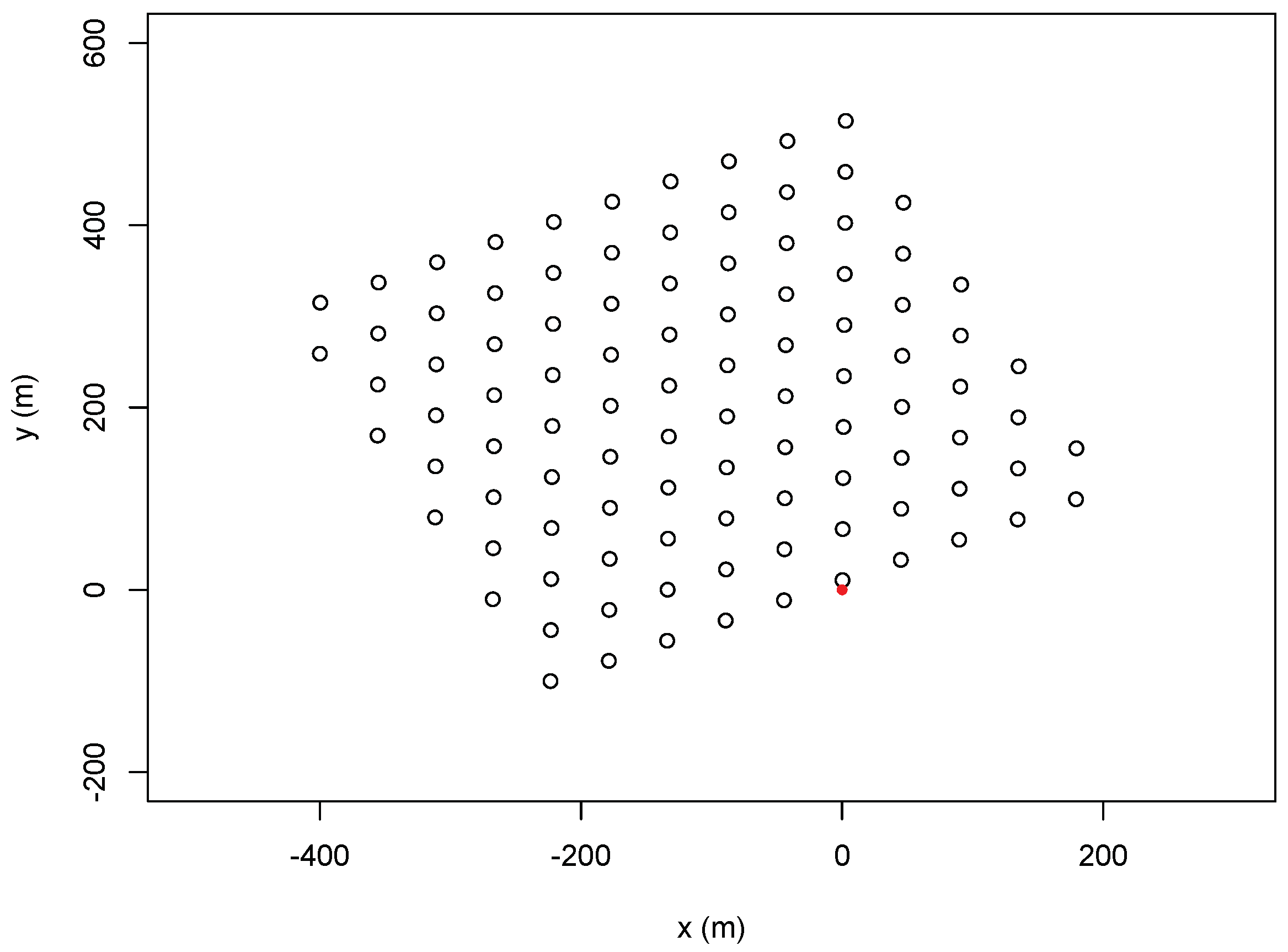
Observations were taken by a set of 100 digital Photo Ionization Detector (PID) samplers, arranged in a rectangular staggered grid/array of area 475 m × 450 m in 10 rows and 10 columns as in Figure 1.

Samplers height is the same as the one of the source and the probe grid was set to $-{25}^{\circ }$ from the north direction in order to take advantage of the prevailing wind flow [23]. PIDs were set in the flattest, most uniform and most homogeneous terrain in order to reduce the effect of the ground level mechanical turbulence. The friction velocity is calculated from the momentum stresses which are in turn calculated from the wind velocity fluctuation components. It is worth to notice that the wind direction in the data set varies during the experiments, which is expected in low-wind speed conditions. However, we use the average value and this may cause some discrepancies between model results and observations.

3. Results

3.1. Statistical Analysis

We firstly analyze the model results concerning the mean concentration. We compare the simulated and observed data (see Section 3.1.1). Then we take into account the fluctuations (concentration variance) simulated by the model and estimate the discrepancies with respect to the observation (see Section 3.1.2). For the statistical analysis, we considered the metrics suggested by [24]: mean value, Fractional Bias (FB), Normalized Mean Square Error (NMSE), correlation coefficient (R), Factor of two (FAC2) and Factor of five (FAC5). If $x_m$ indicates the measured and $x_c$ the calculated values, they are defined as follows,

$$FB=2\frac{{\overline{x}}_m-{\overline{x}}_c}{{\overline{x}}_m+{\overline{x}}_c}$$

(8)

that indicate overestimation if $FB<0$ or underestimation if $FB>0$;

$$NMSE=\frac{\overline{{(x_m-x_c)}^2}}{{\overline{x}}_m{\overline{x}}_c}$$

(9)

where overline indicates the mean; FAC2 is the fraction of data that satisfy

$$0.5⪕\frac{x_c}{x_m}⪕2,$$

(10)

while FAC5 is the fraction of data that satisfy

$$0.2⪕\frac{x_c}{x_m}⪕5.$$

(11)

3.1.1. Mean Concentration

In order to evaluate the agreement between model results and observations, we sort the trials in different groups on the basis of the stability conditions. Then, we perform the statistical analysis separately on each group of trials.

Stable Condition Trials

All trials carried out in stable conditions are examined together. The first simulation is carried out using the [18] parameterization for the turbulence variances and Lagrangian time-scales. The results show that the model is unable to correctly simulate the mean concentrations at the most distant samplers. It may be noted that the parameterizations of the standard deviation and the Lagrangian time-scales are derived for the boundary layer scale. It is likely that they cannot reproduce carefully the turbulence at a such small scale as the one of this experiment which is of the order of a few hundred meters. As a consequence, also the dispersion is not properly simulated and the mean concentrations are underestimated, which can be due to values of the higher values of the turbulence parameters. On the other hand, we observe that the number of samplers reached by the plume in the simulations is lower compared to the one observed in the experiment. This is clearly due to the limited horizontal dispersion. To overcome these problems, we modify the original parameterization reducing either ${\sigma }_w$ or $T_{L_w}$ values in order to limit the underestimations of the mean concentrations, and increasing either ${\sigma }_v$ or $T_{L_v}$ values with the aim of increasing the horizontal dispersion. After different tests, performed by varying the numerical coefficients, we obtain the best results with the following two schemes:

• (Sa) ${\sigma }_v\to {\sigma }_v/0.2$, ${\sigma }_w\to 0.2{\sigma }_w$
• (Sb) $T_{L_v}\to T_{L_v}/(m_s/\overline{U})$, $T_{L_w}\to (m_s/\overline{U})T_{L_w}$

where $\overline{U}$ is the mean wind speed, $m_s$ = 0.03 m/s is a suitable coefficient and ${\sigma }_w$, $T_{L_w}$, ${\sigma }_v$ and $T_{L_v}$ vertical profiles are given by [18] parameterizations.

Table 1. Statistical analysis for the mean concentrations in the stable cases.

Stable Condition Trials
Coefficients	Mean m (g/m${}^3$)	Mean c (g/m${}^3$)	FB	NMSE	R	FAC2 (%)	FAC5 (%)
Hanna base	$0.0028$	$0.0014$	$0.67$	$4.79$	$0.06$	$0.00$	20
Hanna (Sa)	$0.0028$	$0.0020$	$0.33$	$3.78$	$0.04$	$0.00$	33
Hanna (Sb)	$0.0028$	$0.0009$	$1.00$	$87.33$	$-0.02$	$0.00$	26

reports the statistical analysis for the mean concentrations in the stable cases. It can be observed that the parameterization Hanna (Sa) gives the best results. Both FB and NMSE are reduced with respect to the base parameterization, while FAC5 increases. There are not improvements concerning R and FAC2. On the contrary, the parameterization Hanna (Sb) does not show any improvement with respect to the base one.

It is worth mentioning that as the best results we mean that it is the best among those we tested. As, for example, by modifying standard deviations and Lagrangian time-scales with different coefficients or modifying the standard deviations as a function of the wind speed. The idea to use the mean flow to modify the turbulence parameters is an attempt to provide a general method that can be applied in different cases without using ad hoc coefficients. It is likely that the Lagrangian time-scales may be larger when the mean flow is weak due to effects like meandering which maintains the velocities correlated for longer time. Generally, the poor results may be in agreement with the findings of Mortarini et al. [25] which show that in low wind speed and stable conditions the Hanna parameterization underestimates the horizontal Lagrangian time-scales, while it overestimates the vertical one.

Neutral Condition Trials

The two neutral trials, trials 14 and 46, are studied separately. As in the case of stable trials, the model, using the [18] parameterization, tends to underestimate the farthest measurements. For this reason, we modified this parameterization, in order to decrease the vertical dispersion and increase the horizontal one, as follows:

• (Na) ${\sigma }_v\to {\sigma }_v/0.2$, ${\sigma }_w\to 0.2{\sigma }_w$ (a)
• (Nb) ${\sigma }_v\to {\sigma }_v/(m_s/\overline{U})$, ${\sigma }_w\to (m_s/\overline{U}){\sigma }_w$

where $\overline{U}$ is the mean wind speed and, in this case, $m_s$ = 0.01 m/s. Additionally, in this case we try to obtain a general expression by introducing the dependency on the mean wind. In low-wind speed conditions the thermal turbulence, that in neutral conditions is weak, is increased with respect to mechanical turbulence and the vertical variance is higher. The horizontal standard deviation decreases of the same quantity in order to preserve the plume section size. Generally, mean flow is of the order of one thus the standard deviations in the Nb parameterization are varied of about one order of magnitude with respect to the Na parameterization which also allows assessing the sensitivity of the model to the parameterization. Results are shown in

Table 2. Statistical analysis for the mean concentrations in the neutral case trial 14. m indicates measured and c calculated.

Trial14 (Neutral)
Coefficients	Mean m (g/m${}^3$)	Mean c (g/m${}^3$)	FB	NMSE	R	FAC2 (%)	FAC5 (%)
Hanna base	$0.0012$	$0.0007$	$0.53$	$14.89$	$0.28$	11	33
Hanna (Na)	$0.0012$	$0.0013$	$-0.10$	$6.50$	$0.28$	22	61
Hanna (Nb)	$0.0012$	$0.0014$	$-0.21$	$6.49$	$0.40$	17	33

and

Table 3. Statistical analysis for the mean concentrations in the neutral case trial 46. m indicates measured and c calculated.

Trial46 (Neutral)
Coefficients	Mean m (g/m${}^3$)	Mean c (g/m${}^3$)	FB	NMSE	R	FAC2 (%)	FAC5 (%)
Hanna base	$0.0023$	$0.0009$	$0.91$	$16.18$	$0.44$	7	14
Hanna (Na)	$0.0023$	$0.0019$	$0.21$	$6.80$	$0.45$	12	45
Hanna (Nb)	$0.0023$	$0.0019$	$0.21$	$5.23$	$0.62$	17	29

.

Looking at Table 2, where the results of the statistical analysis for trial 14 are presented, it can be observed that, while the base parameterization underestimates the observations (positive FB), both the modified parameterizations slightly overestimate the measured values (negative FB). Hanna (Na) improves both FAC2 and FAC5, while Hanna (Nb) provides a slightly higher value for R.

In the case of trial 46 (Table 3) both the modified parameterizations show an improvement of the results: FB and NMSE decrease with respect to the base parameterization, R increases in the case of Hanna (Nb) parameterization; FAC2 and FAC5 are better in both the cases and particularly concerning FAC5 in the case of Hanna (Na) parameterization.

Unstable Conditions Trial

The unstable condition trial 45 analysis provides a rather good agreement with observed data. For this reason, we do not modify the original [18] parameterization. The results of the statistical analysis are shown in

Table 4. 45. m indicates measured and c calculated.

Trial45 (Unstable)
Coefficients	Mean m (g/m${}^3$)	Mean c (g/m${}^3$)	FB	NMSE	R	FAC2 (%)	FAC5 (%)
Hanna base	$0.0001$	$0.0009$	$-1.58$	$8.82$	$0.93$	17	58

.

The performance of the model is generally satisfactory, particularly for R and FAC5. The FB value shows that the observations are slightly overestimated.

3.1.2. Concentration Variance

As said in Section 2, in order to simulate the turbulent transport of the concentration variance, we need to prescribe the dissipation time-scale. Dissipation is supposed to be caused by energy transfer from large scales to smaller ones on to viscosity, as observed by Richardson (1922) [26]. In terms of time-scale, it can be related to Lagrangian time-scale. For this reason, the dissipation time-scale is supposed to be proportional to the vertical Lagrangian time-scale, which is the most relevant direction in the boundary layer:

$$t_d\left(\mathbf{r}\right)=A{T}_{L_W}\left(z\right),$$

(12)

where the coefficient A should be parameterized. Following Ferrero (2017) [16], this coefficient is linear with mean wind direction coordinate x and depends on the height $H_s$ and diameter $d_s$ of the physical source:

$$A(\mathbf{r},t)=A_1\frac{x}{H_{mix}}+A_2{\left(\frac{d_s}{H_s}\right)}^{\frac{1}{3}},$$

(13)

where $A_1=73.3$ and $A_2=1.25$. The results are presented in terms of concentration standard deviation.

As said in Section 2, to calculate the sources of variance, the model needs a mean concentration field. Thus, we used the previous analysis to select the proper turbulence parameterization for the different trials. For the trials carried out in stable conditions we use the Hanna (Sa) parameterization, for those in neutral condition the Hanna (Nb) parameterization is selected while in the unstable case the Hanna base is the only parameterization tested. It is worth mentioning that the same model and consequently the same parameterization are used to simulate both mean concentration and variance concentration fields.

Stable Conditions Trials

The results for stable cases are presented in

Table 5. Statistical analysis for the mean concentration and the concentration standard deviation in the stable cases. m indicates measured and c calculated.

Stable Condition Trials
	Mean m	Mean c	FB	NMSE	R	FAC2	FAC5
	(g/m${}^3$)	(g/m${}^3$)				(%)	(%)
MEAN	$0.0028$	$0.0020$	$0.33$	$3.78$	$0.04$	0	33
STD	$0.0076$	$0.0023$	$1.08$	$84.00$	$0.01$	21	44

. For the sake of clarity, in the following tables also the mean concentration (MEAN) performance is reported. The value of FB shows that the observations are overall underestimated, less than a factor of two for the MEAN and more than a factor of three for standard deviation (STD). The NMSE is lower for mean concentration with respect to those for concentration standard deviation. FAC2 and FAC5 are rather low, but slightly higher for the concentration standard deviation.

Neutral Conditions Trials

In

Table 6. Statistical analysis for the mean concentration and the concentration standard deviation in the neutral case trial 14. m indicates measured and c calculated.

Trial14
	Mean m	Mean c	FB	NMSE	R	FAC2	FAC5
	(g/m${}^3$)	(g/m${}^3$)				(%)	(%)
MEAN	$0.0012$	$0.0014$	$-0.21$	$6.49$	$0.40$	17	33
STD	$0.0023$	$0.0058$	$-0.86$	$7.99$	$0.33$	6	17

and

Table 7. Statistical analysis for the mean concentration and the concentration standard deviation in the neutral case trial 46. m indicates measured and c calculated.

Trial46
	Mean m	Mean c	FB	NMSE	R	FAC2	FAC5
	(g/m${}^3$)	(g/m${}^3$)				(%)	(%)
MEAN	$0.0023$	$0.0019$	$0.21$	$5.23$	$0.62$	17	29
STD	$0.0059$	$0.0022$	$0.89$	$6.02$	$0.54$	12	24

, the statistical analysis for the two neutral cases is shown. The performances of the model in two cases are very similar, both for the mean concentration and the concentration standard deviation. However, we observed that in the trial 14 the MEAN is correctly reproduced, while STD is overestimated by about a factor of three. In the trial 46, MEAN shows a good agreement while STD is underestimated of about a factor of three. The values of R are better for the trial 46 with respect to trial 14.

Unstable Conditions Trial 45

Both MEAN and STD are overestimated by about a factor of 10, as shown by the FB value and the means (see

Table 8. Statistical analysis for the mean concentration and the concentration standard deviation in the unstable case trial 45. m indicates measured and c calculated.

Trial45
	Mean m	Mean c	FB	NMSE	R	FAC2	FAC5
	(g/m${}^3$)	(g/m${}^3$)				(%)	(%)
MEAN	$0.0001$	$0.0009$	$-1.58$	$8.82$	$0.93$	17	58
STD	$0.0005$	$0.0052$	$-1.68$	$14.10$	$0.16$	17	42

). Both NMSEs are quite high meaning that the error is significant. R is close to 1 for mean concentration value, which indicates that there is strong correlation between simulated and observed data. On the contrary, for STD, R is very low. FAC2 is low for both the quantities while FAC5 being about 50% for both quantities shows a consistent amount of measured data is not too far from their respective observed ones.

3.2. Graphical Analysis

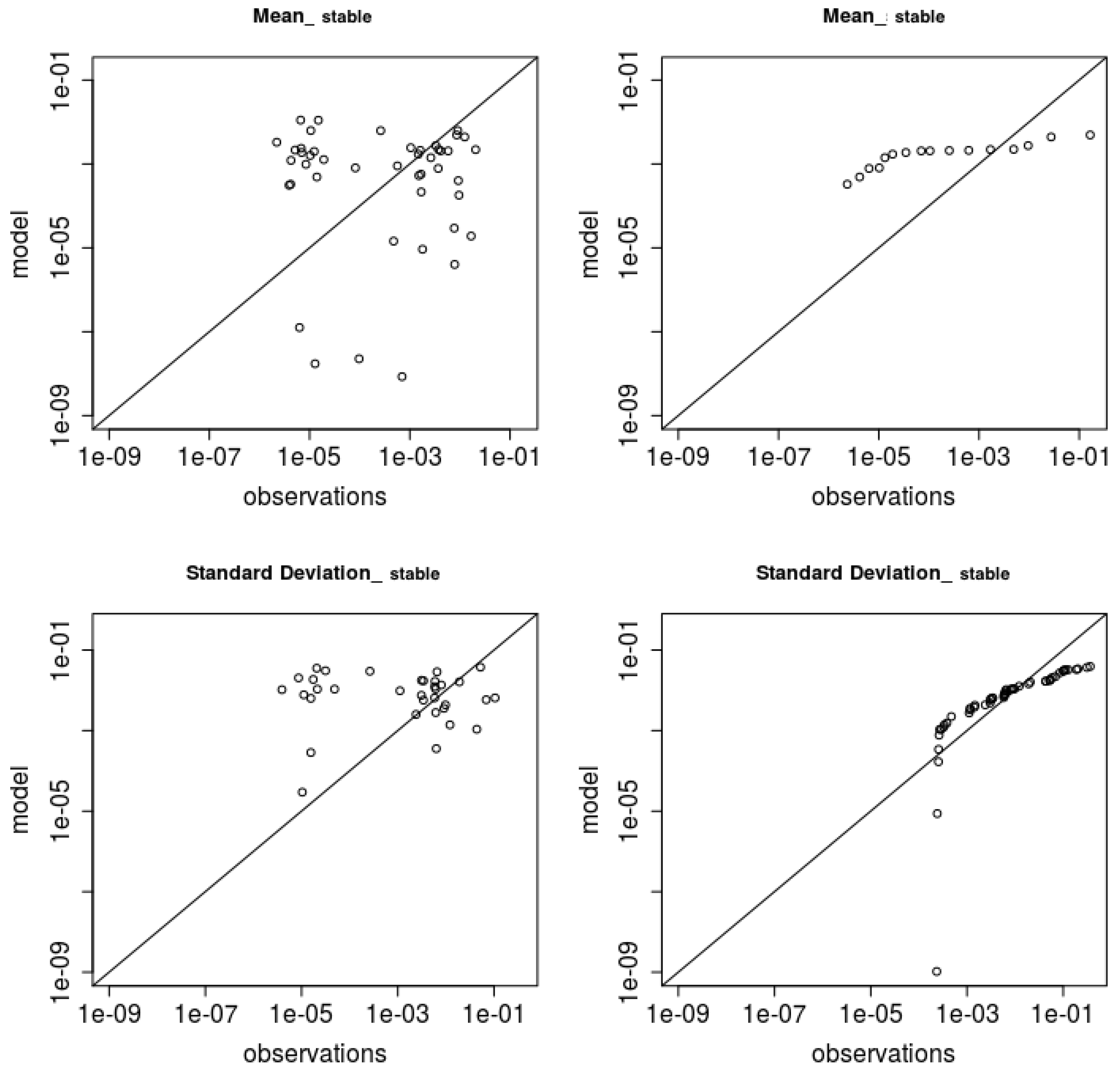
The following plots show the comparison between simulated and observed data by means of scatter-plot and qq-plot in logarithmic scale. The former compares each measured value (x-axis) with its respective observed one (y-axis), while the second displays quantile accordance. In the qq-plots, we paired the predicted and observed values from the lowest ones to the highest ones, while in the scatter plots the values are paired depending on the probe position. In this way, some of the points in the plots may not appear since one of the two values (either predicted or observed) is zero or below the plot limits. However, this may occur for different points in the qq-plots or in the scatter-plots. In the statistical analysis, zero values are included except for the calculation of FAC2 and FAC5 in which we exclude the measured zero values.

3.2.1. Stable Condition Trials

All stable trial results are shown in Figure 2. As far as the mean concentration is considered, it can be observed that the model overestimates the lower values, while it underestimates the higher ones. The concentration standard deviations provide a satisfactory performance for the higher values and generally when considering the quantiles.

3.2.2. Neutral Condition Trials

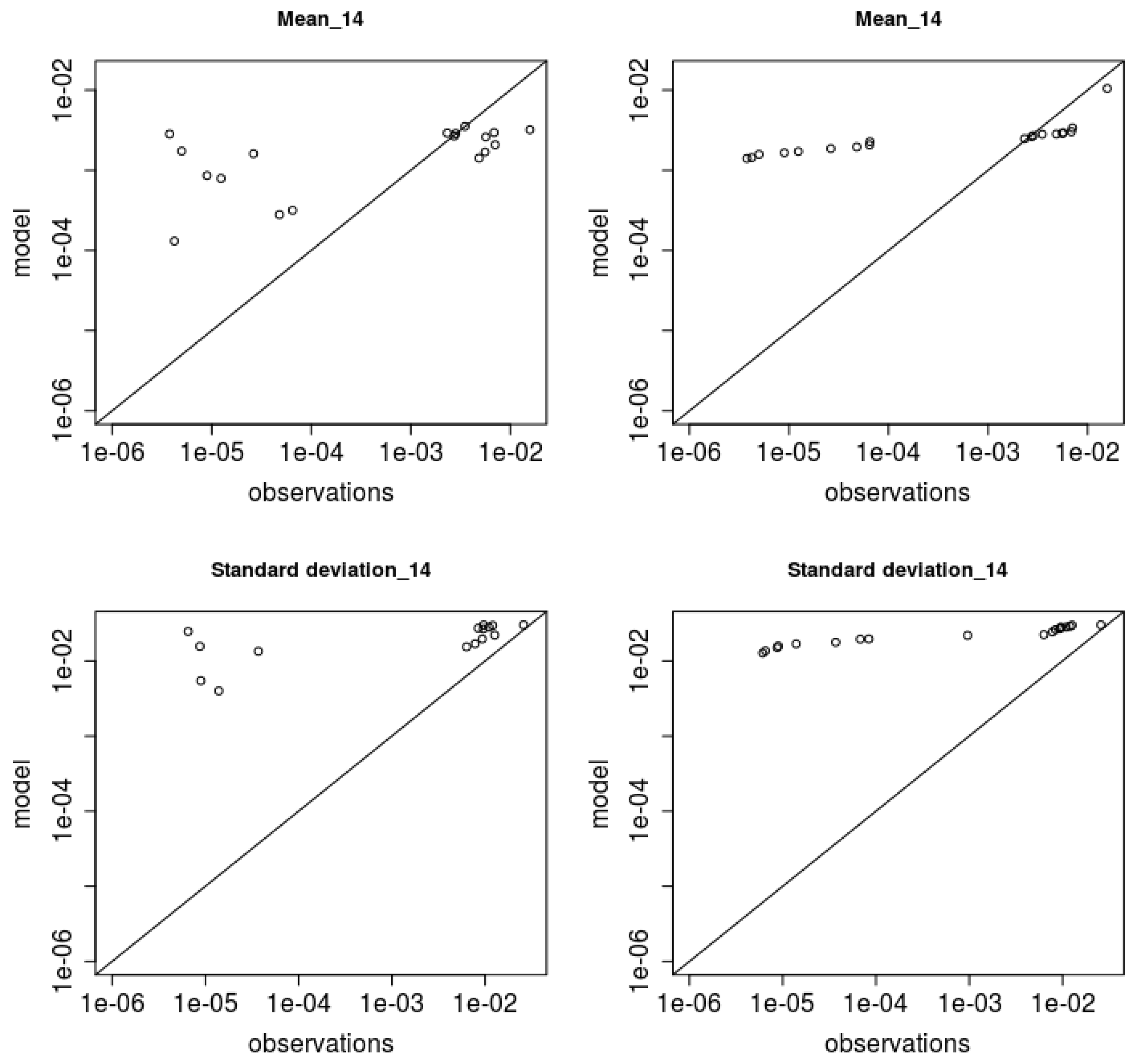
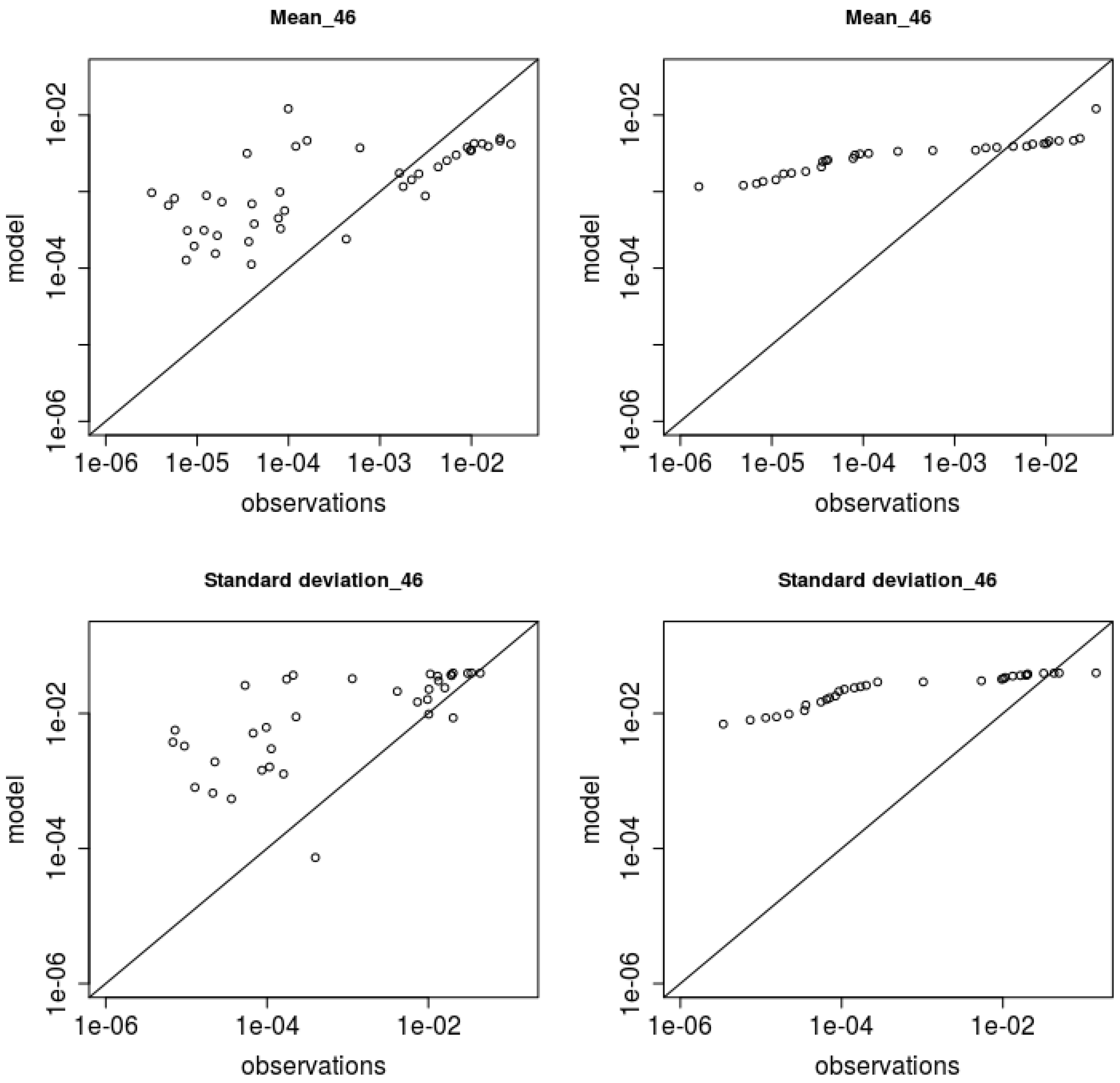
Neutral trials have been studied separately. Both mean concentration and concentration standard deviation lower values for trial 14 (Figure 3) are overestimated, while the higher values are better captured. Similar results are obtained for the trial 46 (Figure 4).

3.2.3. Unstable Condition Trial 45

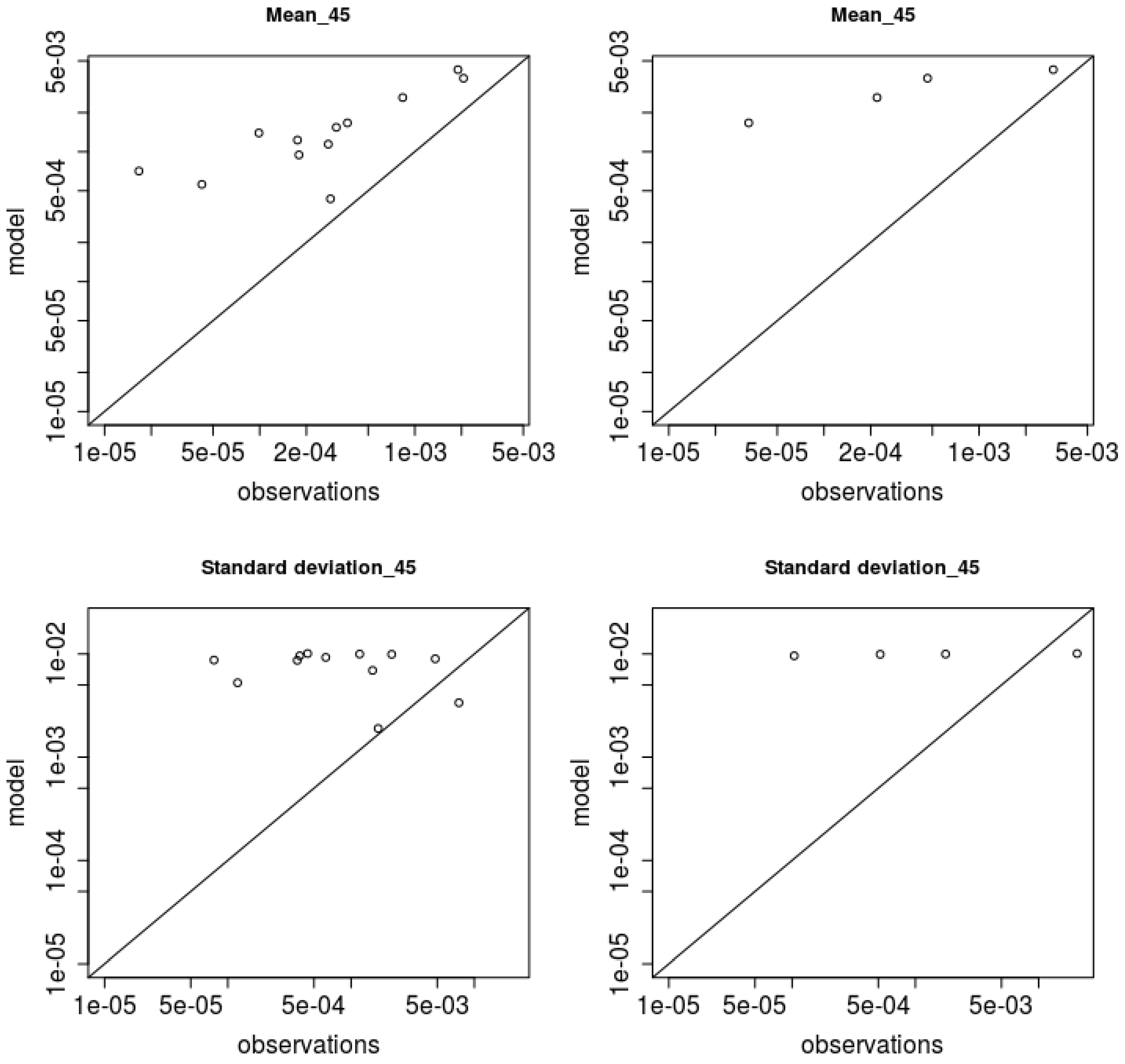
The trial 45 refers to unstable conditions. The results are shown in Figure 5. Both mean concentration and concentration standard deviations values are overestimated. The mean concentration seems to be more correlated with respect to the concentration standard deviations. Both qq-plots for mean concentration and concentration variance show low quantile agreement with basically every value being overestimated.

4. Conclusions

A Lagrangian stochastic model is tested against data measured in a field experiment. Both mean concentrations and concentration standard deviations dispersion were simulated and the results compared against the observations. We found that the [18] parameterizations should be changed in order to proper simulate the mean concentration dispersion in stable, as already noted by [27,28], and neutral conditions, while in unstable conditions they give satisfactory results. It may be worth noticing, that the scales of the experiment are very small, a few hundred meters and about 10 min, which are very different from those of the typical dispersion in the atmospheric boundary layer.

As a matter of fact, in this space-time domain the usual parameterizations, that are designed for larger scales and for stationary conditions, do not allow to simulate the dispersion correctly and, as a consequence, many measurement points are not reached by the simulated plume.

The modification in the original parameterizations is aimed at increasing the horizontal dispersion and decreasing the vertical one. It can be noted that, in this way, the plume section size is preserved. Therefore a result of this work is that modifications of turbulence parameterizations are needed when simulations are performed on scales of a few hundred meters and minutes.

Comparing the results that we obtain for the mean concentrations using Hanna (Sa) parameterization with those estimated by [23], that evaluated the performance of a number of dispersion schemes for this data set, we can observed that in the case of stable conditions NMSE is of the order of the best values found in that paper, while FB is in the middle of the range of values obtained by [23]. On the contrary, the FAC2 that we found is worse. Concerning the unstable conditions, our results are worse with respect to those of [23] except for one of the parameterizations that they took into account.

The same parameterizations that we use for the mean concentrations are applied in simulating the concentration standard deviation dispersion giving results that can be considered satisfactorily at least in the stable conditions. For other stability conditions, more research is still needed to account for proper parameterizations which allow to correctly reproduce the observations. The results of this work show that the method proposed for the simulation of concentration variances, taking into account the severity of the experiment considered for comparison, is promising. The results for the stable cases are quite good, while in the neutral and unstable cases the analysis of turbulence parameterizations for the small scale needs to be further investigated.

We can conclude that the approach suggested firstly by [14] and later by [16,17,29] can be applied at such a small scale in different stability conditions and low-wind conditions. It is worth to notice that such challenging conditions can be often related to accidental releases of flammable or explosive gases where the concentration fluctuations should be estimated in order to avoid possible dangerous fires. Finally, we would like to stress that the parameterization for the variance dissipation has been used in previous work [17] but in different conditions. In that case, the stability was neutral in all the experiments and the wind ranged from 2.5 to 7.9 m/s while in the present experiments we have all the stability conditions and very weak wind ranging from 1.2 to 2.7 m/s. It is well-known that these conditions are much more challenging with respect to the case of neutral conditions and strong wind.

References

1. Hinze, J. Turbulence; McGraw Hill Book Co. Inc.: New York, NY, USA, 1959. [Google Scholar]
2. Gifford, F. Statistical properties of a fluctuating plume dispersion model. Adv. Geophys. 1959, 6, 117–137. [Google Scholar]
3. Franzese, P.; Borgas, M. A simple relative dispersion model for concentration fluctuations in clouds of contaminant. J. Appl. Meteorol. 2002, 41, 1101–1111. [Google Scholar] [CrossRef]
4. Franzese, P. Lagrangian stochastic modeling of a fluctuating plume in the convective boundary layer. Atmos. Environ. 2003, 37, 1691–1701. [Google Scholar] [CrossRef]
5. Yee, E.; Gailis, R.; Wilson, D. The Interference of Higher-Order Statistics of the Concentration Field Produced by Two Point Sources According to a Generalized Fluctuating Plume Model. Boundary-Layer Meteorol. 2003, 106, 297–348. [Google Scholar] [CrossRef]
6. Gailis, R.M.; Hill, A.; Yee, E.; Hilderman, T. Extension of a fluctuating plume model of tracer dispersion to a sheared boundary layer and to a large array of obstacles. Boundary-Layer Meteorol. 2007, 122, 577–607. [Google Scholar] [CrossRef]
7. Mortarini, L.; Franzese, P.; Ferrero, E. A fluctuating plume model for concentration fluctuations in a plant canopy. Atmos. Environ. 2009, 43, 921–927. [Google Scholar] [CrossRef]
8. Ferrero, E.; Mortarini, L.; Alessandrini, S.; Lacagnina, C. Application of a Bivariate Gamma distribution for a chemically reacting plume in the atmosphere. Bound-Layer Meteorol. 2013, 147, 123–137. [Google Scholar] [CrossRef]
9. Durbin, P.A. A stochastic model of two particle dispersion and concentration fluctuation in homogeneous turbulence. J. Fluid Mech. 1980, 100, 279–302. [Google Scholar] [CrossRef]
10. Thomson, D.J. A stochastic model for the motion of particle pairs in isotropic high Reynolds number, and its application to the problem of concentration variance. J. Fluid Mech. 1990, 210, 113–153. [Google Scholar] [CrossRef]
11. Ferrero, E.; Mortarini, L. Concentrations fluctuations and relative dispersion PDF. Atmos. Environ. 2005, 39, 2135–2143. [Google Scholar] [CrossRef]
12. Mortarini, L.; Ferrero, E. A Lagrangian stochastic model for the concentration fluctuations. Atmos. Chem. Phys. 2005, 5, 1–10. [Google Scholar] [CrossRef] [Green Version]
13. Ferrero, E.; Manor, A.; Mortarini, L.; Oettl, D. Concentration Fluctuations and Odor Dispersion in Lagrangian Models. Atmosphere 2020, 11, 27. [Google Scholar] [CrossRef] [Green Version]
14. Manor, A. A stochastic single particle Lagrangian model for the concentration fluctuation in a plume dispersing inside an urban canopy. Bound. Layer Meteorol. 2009, 94, 253–296. [Google Scholar] [CrossRef]
15. Csanady, G. Concentration fluctuations in turbulent diffusion. J. Atmos. Sci. 1967, 24, 21–28. [Google Scholar] [CrossRef] [Green Version]
16. Ferrero, E.; Mortarini, L.; Purghè, F. A Simple Parametrization for the Concentration Variance Dissipation in a Lagrangian Single-Particle Model. Bound. Layer Meteorol. 2017, 163, 91–101. [Google Scholar] [CrossRef]
17. Ferrero, E.; Oettl, D. An evaluation of a Lagrangian stochastic model for the assessment of odours. Atmos. Environ. 2019, 206, 237–246. [Google Scholar] [CrossRef]
18. Hanna, S. Applications in Air Pollution Modeling; Springer: Dordrecht, The Netherlands, 1982; pp. 275–310. [Google Scholar] [CrossRef]
19. Joffre, S.; Kangas, M.; Heikinheimo, M. Variability Of The Stable And Unstable Atmospheric Boundary-Layer Height And Its Scales Over A Boreal Forest. Bound. Layer Meteorol. 2001, 99, 429–450. [Google Scholar] [CrossRef]
20. Storwald, D. Detailed Test Plan for the Fusing Sensor Information from Observing Networks (Fusion) Field Trial (FFT-07); Technical Report; Document no. wdtc-tp-07-078; Meteorology Division, West Desert Test Center, U.S. Army Dugway Proving Ground WDTC: Dugway, UT, USA, 2007. [Google Scholar]
21. Platt, N.; Warner, S.; Nunez, S. Evaluation plan for comparative investigation of source term estimation algorithms using FUSION field trial 2007 data. Hrvat. MeteorološKi čAsopis 2008, 43, 224–229. [Google Scholar]
22. Singh, S.; Sharan, M. Simulation of plume dispersion from single release in Fusion Field Trial-07 experiment. Atmos. Environ. 2013, 80, 50–57. [Google Scholar] [CrossRef]
23. Pandey, G.; Sharan, M. Performance evaluation of dispersion parameterization schemes in the plume simulation of FFT-07 diffusion experiment. Atmos. Environ. 2018, 172, 32–46. [Google Scholar] [CrossRef]
24. Chang, J.C.; Hanna, S.R. Air quality model performance evaluation. Meteorol. Atmos. Phys. 2004, 87, 167–196. [Google Scholar] [CrossRef]
25. Mortarini, L.; Ferrero, E.; Falabino, S.; Trini Castelli, S.; Richiardone, R.; Anfossi, D. Low-frequency processes and turbulence structure in a perturbed boundary layer. Q. J. R. Meteorol. Soc. 2013, 139, 1059–1072. [Google Scholar] [CrossRef] [Green Version]
26. Richardson, L. Weather Prediction by Numerical Process; The University Press: Cambridge, UK, 1922. [Google Scholar]
27. Luhar, A.K. Estimating Variances of Horizontal Wind Fluctuations in Stable Conditions. Bound. Layer Meteorol. 2010, 135, 301–311. [Google Scholar] [CrossRef]
28. Trini Castelli, S.; Falabino, S.; Mortarini, L.; Ferrero, E.; Richiardone, R.; Anfossi, D. Experimental investigation of surface-layer parameters in low wind-speed conditions in a suburban area. Q. J. R. Meteorol. Soc. 2014, 140, 2023–2036. [Google Scholar] [CrossRef] [Green Version]
29. Oettl, D.; Ferrero, E. A simple model to assess odour hours forregulatory purposes. Atmos. Environ. 2017, 155, 162–173. [Google Scholar] [CrossRef]
Figure 1. Experimental set−up: the open circles indicate the probe positions and the red dot the source position. x−axis is directed from west to east, y−axis is directed from south to north.
Atmosphere 12 00589 g001
Figure 2. Scatter-plot (left) and qq-plot (right) for stable condition trials (g m 3 ).
Atmosphere 12 00589 g002
Figure 3. Scatter-plot (left) and qq-plot (right) for trial 14 (neutral conditions) (g m 3 )
Atmosphere 12 00589 g003
Figure 4. Scatter-plot (left) and qq-plot (right) for trial 46 (neutral conditions) (g/m 3 ).
Atmosphere 12 00589 g004
Figure 5. Scatter-plot (left) and qq-plot (right) for trial 45 (unstable conditions) ( g / m 3 )
Atmosphere 12 00589 g005