Article

An Urban Lagrangian Stochastic Dispersion Model for Simulating Traffic Particulate-Matter Concentration Fields

Applied Mathematics Department, Israel Institute for Biological Research, P.O. Box 19, Ness-Ziona 7410001, Israel
*
Authors to whom correspondence should be addressed.
Atmosphere 2021, 12(5), 580; https://doi.org/10.3390/atmos12050580
Submission received: 17 March 2021 / Revised: 22 April 2021 / Accepted: 25 April 2021 / Published: 30 April 2021
(This article belongs to the Special Issue Air Pollution and Human Exposures in Israel)

Abstract

:
The accumulated particulate matter concentration at a given vertical column due to traffic sources in urban area has many important consequences. This task, however, imposes a major challenge, since the problem of realistic pollutant dispersion in an urban environment is a very demanding task, both theoretically and computationally. This is mainly due to the highly inhomogeneous three dimensional turbulent flow regime in the urban canopy roughness sublayer, which is far from “local equilibrium” between shear production and dissipation. We present here a mass-consistent urban Lagrangian stochastic model for pollutants dispersion, where the flow field is modeled using a hybrid approach by which we model the surface layer based on the typical turbulent scales, both of the canopy and in the surface layer inertial sub-layer. In particular it relies on representing the canopy aerodynamically as a porous medium by spatial averaging the equations of motion, with the assumption that the canopy is laterally uniform on a scale much larger than the buildings but smaller than the urban block/neighbourhood, i.e., at the sub-urban-block scale. Choosing the spatial representative averaging volume allows the averaged variables to reflect the characteristic vertical heterogeneity of the canopy but to smooth out smaller scale spatial fluctuations caused as air flows in between the buildings. This modeling approach serves as the base for a realistic and efficient methodology for the calculation of the accumulated concentration from multiple traffic sources for any vertical column in the urban area. The existence of multiple traffic sources impose further difficulty since the computational effort required is very demanding for practical uses. Therefore, footprint analysis screening was introduced to identify the relevant part of the urban area which contributes to the chosen column. All the traffic sources in this footprint area where merged into several areal sources, further used for the evaluation of the concentration profile. This methodology was implemented for four cases in the Tel Aviv metropolitan area based on several selected summer climatological scenarios. We present different typical behaviors, demonstrating combination of source structure, urban morphology, flow characteristics, and the resultant dispersion pattern in each case.

1. Introduction

There are a considerable number of studies that point out the hazard to health following exposure to traffic-related PM 10 . Specifically, such exposure was found to be associated with adverse changes in the regulation of the cardiovascular system among subjects without cardiovascular disease [1], risk of asthma development among children [2] and incidence rates of lung cancer among males [3,4]. Several campaigns were held in different urban regions around the world in which particulate matter concentrations were measured in different heights, ranging from ground level up to several hundreds of meters above ground. All these have exhibited variability in the PM 10 vertical concentrations [5,6,7]. This variability lead some authors to try and quantify the level of exposure to traffic related PM 10 as a function of the height of residence [8]. Therefore, in order to realistically assess the exposure to traffic-related PM 10 in an urban environment it is imperative to simulate quantitatively the three dimensional PM 10 concentration field.
Realistic modeling of transport and dispersion of pollutants at the city scale is a very challenging problem due to the non-uniform and complex nature of the flow field within and just above the canopy [9,10]. In such environments, the flow structure in the roughness sublayer (RSL) dictates the air flow and pollutant dispersion within and above urban canopies. This sub-layer consists of the lowest part of the atmospheric surface layer, from the ground to 2–5 average height of the canopy elements. Moreover, the RSL is where the turbulent exchange of momentum, heat and mass occur [9,11]. The main important flow features are the shear layer generated at the roof-top level as well as the highly inhomogeneous turbulent flow within the urban canopy [12,13]. The thickness of the shear layer depends on the averaged morphological parameters (e.g., the packing density) of the canopy elements [14,15]. Furthermore, the turbulent kinetic energy (TKE) budget, well above the canopy, reduces to a “local equilibrium” between shear production and dissipation, and therefore can be approximated in terms of Monin-Obukhov similarity theory (MOST) [9,16]. On the other hand, within and just above the canopy, due to locally generated turbulence, the entire canopy flow is far from the “local-equilibrium” [11,17].
Over the past few decades an effort was made to model realistic dispersion of pollutants at the urban scale (see, e.g., overview in [18]). Few attempts were made when the emphasis was on quantitative models. When efficiency was also a focus these attempts were usually based on Lagrangian stochastic models (LSM) for transport and dispersion [19]. LSM is able to describe consistently gas dispersion phenomena in rather complicated atmospheric scenarios such as non-homogeneous turbulent regimes, complex terrain and canopies (urban and vegetation) [20], and is superior to advection-diffusion-based approaches (see e.g., [21,22]). The main methods included: computational fluid dynamics (CFD) simulations around hundreds to thousands of buildings (e.g., [23] and references therein); application of Reynolds-averaged Navier–Stokes (RANS) and large-eddy simulation (LES) complemented by LSM (e.g., [18,24,25]). A third approach is based on evaluating a diagnostic-empirical method [26] and use that to drive LSM [27,28,29]. This approach relys on a consistent mean wind field based on as many as needed urban canyon scale diagnostic-empirical estimates for the different buildings configurations. It was also shown to be practical for planar urban areas but may be too demanding for complex terrain urban areas. The key limitations of the all the above are that of excessive computational demand (due to the mass consistency constraint even for the diagnostic-empirical approach), and often difficulty in extending to more complex and general canopies such as a city scale over complex terrain.
The aim of this study is to employ an efficient and general LSM approach to estimate the accumulated concentrations field from traffic particulate matter pollutants in an urban area at the city scale. To do so, we use an urban LSM developed at the Israeli Institute for Biological research (IIBR) for urban canopy over complex terrain solved at the city scale [30]. The modeling presented in this study is based on spatial averaging of the urban morphology, with the assumption that the canopy is laterally uniform on a scale much larger than the buildings but smaller then the urban neighbourhood/block, i.e., at the sub-urban-block scale. This is achieved by formulating the equations of motion as double (space-time) averaged over the sub-urban-block scale volume, thus representing the urban canopy layer aerodynamically as a quasi-horizontally homogeneous porous medium. Using a spatial representative averaging volume enables the averaged variables to reflect the characteristic vertical heterogeneity of the canopy. Moreover, it allows smoothing out smaller scale spatial fluctuations that are generated as wind flows in between the buildings, while maintaining the effect of the turbulent exchange of the canopy (e.g., [15,31]).
To calculate the accumulated concentration at a given vertical column in the urban area, we first use footprint analysis [32,33] to locate the dimensions of the source area with respect to the influence on concentration at the requested column, then calculate the sources in this footprint as local areal sources. From each areal source and averaged morphological parameters we analyse the accumulation of pollutant field for a given vertical column. This approach enables a significant reduction of required LSM simulations, which makes it efficient for cases where multiple sources are essential. This method was implemented for four test cases in the Tel Aviv metropolitan area that occur during the typical rush-hour periods.

2. Theory and Methods

2.1. The Lagrangian Stochastic Model

To evaluate the concentration field of pollutant at the POI, one has to specify the underlying turbulent pollutant dispersion model. In this study, a mass-consistent Lagrangian stochastic model (LSM) for urban canopy over complex terrain developed at the Israeli institute for biological research (IIBR) [30], has been used. Its details, for the case of dispersion within and above urban canopy under near neutral conditions, are outlined in this section. This model was formulated for urban canopy including over complex terrain, and was validated against urban atmospheric tracer release field campaign in the city of Haifa (on the Camel mountain), Israel, exhibiting full compliance with all statistical acceptance criteria for urban dispersion models [30] (see also [34,35]).
The LSM approach is based on modelling turbulent dispersion as a first-order Markov process with the velocity-displacement conditional distribution function as the principal characteristic of the motion in Lagrangian variables, while maintaining consistency with the Kolmogorov 1941 similarity theory [36]. For homogeneous isotropic turbulence, this approach is well-established (e.g., [37]; for an analytical solution see e.g., [21] (suppl.)), however, a unique expression valid for general anisotropic inhomogeneous turbulence is missing. A model for inhomogeneous turbulence is formulated based on a necessary condition called the well-mixed condition, which assures consistency with the second law of thermodynamics [19]. This condition allows the use of a pre-assumed one-particle Eulerian velocity probability distribution function (PDF), but was found to be necessary but not sufficient, except for the one-dimension case. Moreover, this one-particle LSM approach, which deals with absolute dispersion in a fixed reference frame and the mean concentration field, is able to describe consistently passive scalar dispersion phenomena, in complicated atmospheric scenarios such as non-homogeneous turbulent regimes, complex terrain and canopies [20].
The velocity perturbation u i ( i = u , v , w ) at the particle position x p = x i and time t about the local mass consistent Eulerian mean velocity U E i (instead of the Lagrangian) can be written as U E i ( x p , t ) + u i ( x s , t ) ( x s is the source position), e.g., [38,39]. Therefore, we formulate the first-order Lagrangian stochastic process by calculating the Lagrangian trajectories of fluid parcels (referred to as ’particles’). A ’new’ particle velocity is initiated as a Gaussian random variable of zero average and of variance 2 v i 2 ). These ’particles’ are passively marked at time zero according to a velocity PDF, at the point or volume of the pollutant source. This leads to the following set of generalized Langevin equations (GLE) for particle displacement and velocity fluctuation/perturbation:
d x i = ( U E i + u i ) d t d u i = a i ( u i , x i ) d t + b i j d W j ( t )
where d W i is an increment of the Wiener process, i.e., Gaussian random variate with average d W i = 0 and variance d W i d W j = d t δ i j [40], and a mass consistent adjusted Eulerian mean velocity field U E i is implemented on surface-following coordinate, obtained using a fast multigrid numerical algorithm [41]. Based on the Kolmogorov 1941 similarity theory for the second-order structure function we get d u i d u j = C 0 ϵ d t δ i j = b i j 2 d t δ i j , where ϵ is the average dissipation rate of the turbulent kinetic energy and C 0 is the so-called Kolmogorov constant [36]. The Kolmogorov 1941 structure function scaling was shown to be valid in recent direct Lagrangian measurements in highly inhomogeneous canopy flow (modeled at the IIBR environmental wind tunnel [42,43]), despite an observed large-scale intermittency which affects the energetics of trajectories [44]. The value of C 0 is known to vary on a broad scale of values between 2–8, see overview in [45], and deduction for canopy flow from direct Lagrangian measurements [13]. Therefore, in order to avoid ‘tweaking’, its specification must be based on relevant observations or modeling. In this study, we use C 0 = 3 , based on [46,47]. It should also be noted that as Du 1997 [46] shows, the mean concentrations are not very sensitive to small changes in C 0 .
The deterministic coefficients a i can be determined via the Fokker-Planck equation, by satisfying Thomson’s well mixed (necessary) condition [19], i.e., by assuming a shape for the one-particle PDF of an Eulerian velocity. The choice of the velocity PDF depends on the statistics of the flow. In an urban canopy, the flow is known to be highly inhomogeneous (e.g., [13]) and is known to exhibit some intermittent higher moments of momentum due to an ejection-sweep burst cycle (e.g., [48]). However, it was shown that when skewness is accompanied with highly inhomogeneous flow, the inhomogeneity dominates. This effect is evident on the canopy scale due to strong multi-axial shear in the mean wind field (e.g., [38]). Moreover, it was shown recently that on the canopy obstacles scale, there exists a rapid decorrelation of the Lagrangian time-scales attributed to the flow disturbances in the obstacles’ wakes, i.e., turbulence-obstacle interaction [13]. This was further shown to lead to a velocity probability function which is well approximated by a one-particle Gaussian Eulerian velocity-fluctuation PDF [13]:
P E = 1 ( 2 π ) 3 / 2 d e t ( τ i j ) 1 / 2 e x p ( 1 2 u i S i j u j )
where S i j = ( τ i j ) 1 and τ i j are the stress matrix elements. By using the Fokker-Planck equation, P E may be considered to be a prescribed property of the turbulence, and therefore constrains a i . The well mixed condition of Thomson [19] is formulated as:
a i P E = 1 2 c 0 ϵ P E u i + ϕ i ( x , u , t ) ; ϕ i u i = P E t x i u i P E
with ϕ i 0 as | u | . Except for the one dimensional case, the vector function ϕ i is not uniquely defined, since a series of solutions can be obtained by adding to it an arbitrary vector function whose divergence in velocity space is zero. We use in this study the particular solution of Thomson termed ’simplest solution’ for the above Gaussian Eulerian velocity-fluctuation P E [19]. This solution rely on the choice that the above condition is satisfied by each component separately. Furthermore, it was found to be the simplest one to fulfil the mean Lagrangian trajectories rotation criterion (also termed the ‘zero-spin’ criterion) [49,50]; and was shown to be unique up to an error of a few percentages in predicted dispersion statistics for shear-induced turbulence [51]. It should be noted that for near neutral stratification, for which the use of a Gaussian PDF of the form as in Equation (2) is known to be a good approximation [20], the non-diagonal elements of the stress matrix cannot be neglected because the correlation between the vertical and horizontal wind fluctuations are crucial for the pollutant dispersion. Hence, the ’simplest solution’ for the drift term for stationary non-isotropic and quasi-homogeneous turbulence (relative to the canopy spatial representative averaging scale) for velocity fluctuations takes the form:
a u = 1 2 ( σ u 2 σ w 2 u * 4 ) b u 2 ( σ w 2 u + u * 2 w ) a v = 1 2 σ v 2 b v 2 v a w = 1 2 ( σ u 2 σ w 2 u * 4 ) b w 2 ( u * 2 u + σ u 2 w ) + 1 2 ( σ u 2 σ w 2 u * 4 ) ( u * 2 σ w 2 z u w + σ u 2 σ w 2 z w 2 ) + 1 2 σ w 2 z
where a transformation to along wind coordinates was used, i.e., taking the y coordinate as perpendicular to the averaged wind direction, U, we get V = u v ¯ = v w ¯ = 0 and u * 2 = u w ¯ . u, v and w are the along wind, cross wind and vertical components of the velocity fluctuations, σ i 2 ( i = u , v , w ) are the corresponding velocity variances, and b u , v , w 2 = C 0 ϵ , with ϵ the average dissipation rate of the turbulent kinetic energy and C 0 the Kolmogorov constant (taken here as 3 as mentioned above). We further note that for homogeneous isotropic turbulence the process is simplified to the standard Ornstein-Ohlenbeck process (e.g., [40]).

2.2. Inertia Effects

Modelling atmospheric transport and dispersion of aerosols below 20 μ m using the Lagrangian stochastic approach was used in several studies. Usually, the aerosol was modeled as a passive tracer (e.g., [52,53]). However, some studies accounted for physical and biological phenomenon that affect aerosols [54,55].
In this study, we are interested in the concentrations of PM 10 pollutants in air as they disperse within and above urban canopy. Since the scale of dispersion is of a few tens of kilometers (urban area scale), PM 10 particles originating from traffic (the density depends on the engine’s load and ranges between 0.8–2 g/cm 3 [56]) can be assumed as tracers i.e., inertia effects are negligible. This is assumption can be justified by the following: for traffic pollutants the spatial maps of PM 10 concentrations was found to exhibit similarity with the gas N O x pollutants [4]; from theoretical view point it can be shown by inspecting the ratio of aerosol diffusion coefficient K z to gas diffusion coefficient K z g [57] that for PM 10 which exhibit densities of the order of 2 g/cm 3 the ratio is approximately unity (up to less than 0.1 % ), i.e., inertial effects are negligible.

2.3. Canopy and Surface Layer Modeling

Presently, the accepted picture of the canopy RSL flow (e.g., [11]) is based on the deduction that canopy turbulent flow is dominated by large canopy-scale eddies, whose source is an inviscid instability of the inflected mean velocity profile, just above the canopy. This instability is formed when momentum is absorbed over a significant height range as opposed to a plane surface in a conventional boundary layer. The canopy inflected turbulence structure is analogous to a plane mixing layer, whereas above it, the turbulent flow gradually submerges to an inertial sublayer, similar to a conventional wall-bounded boundary layer [17].
Regarding scales, in the conventional inertial sublayer turbulence scales with z + d , being the displaced distance from the ground origin (in this notation h c is the canopy height and z = 0 at the top of the canopy such that h c z , and d is the displacement distance from ground taken here as 0.7 H c [58]). In addition, in the canopy, as in a plane mixing layer, canopy turbulence has a constant length scale. The transition between these two regimes occurs within the RSL. Above the canopy we adopt the logarithmic form as the wind profile for neutral stratification [59].
To model the actual effect of the canopy drag on the flow and turbulent exchange of the canopy we need a canopy model. As a model for the canopy, based on [15,60], we adopt an approach by which the canopy is treated as patches of porous media, on the canopy sub-urban-block horizontal heterogeneity scale, to which the flow adjusts. This approach is based on a solution of the doubly averaged (time-space) one-dimensional momentum equation, τ z U 2 L c = 0 , with τ being the turbulent shear stress, F D = U 2 / L c the kinematic drag, L c = ( c d a ) 1 the average canopy-drag length scale with dimensionless drag coefficient c d and a being the effective frontal element-area per unit volume. Furthermore, the average canopy-drag length scale L c is modeled based on the averaged morphological scales, L c h c ( 1 λ p ) λ f [15] (assuming constant c d 2 for urban canopy [61]), where λ f is the frontal area density ratio, λ p the plan area density is the ratio of the occupied and total plan area (also termed the solid porosity λ p = 1 ϕ , where ϕ is the air porosity), and h c is the plan area weighted average building height [14]. Analogously we can view the canopy in terms of its porosity, in which case L c can be shown to be proportional to the canopy height h, solid porosity λ p = 1 ϕ and inversely proportional to the frontal area index λ f , i.e., L c ( ϕ h ) / λ f . This also reflects on the canopy boundary conditions which due to its porous nature can be treated as reflective from the ground.
This approach is able account for inhomogeneous canopies, as when the averaged characteristics of the canopy elements vary in space, the canopy length scale, L c , vary as well. Another issue is the distance of adjustment of a sparse/rural boundary layer to a urban canopy of typical density, i.e., the fetch needed for the wind to adjust to such a canopy. It was shown that the winds within the urban canopy adjust after a distance x 0 = 3 L c l n K [61], where the factor l n K ( K = ( U h / U ) ( h c / L c ) , with U h = U ( z = 0 ) the mean wind speed at the top of the canopy) depends on upwind conditions and less on local canopy parameters, and varies between 0.5 and 2 for typical urban settings. Thus, the density and shape of buildings within a radius x 0 only determine the local canopy winds. In this sense x 0 gives a dynamical definition of the size of a neighbourhood [61].
The modeling approach for inhomogeneous urban canopy used here is based on the assumption that the whole city is composed of many smaller patches, each being approximately homogeneous [31]. Based on this approach the horizontal averaging area has dimensions of L A × L A , where the length scale L A over which spatial averaging is performed must be larger than the building spacing but less than the length scale x 0 over which the flow is evolving. Thus, we have to assert that a scale separation exists between these two length scales in order to implement this model. Such assertion is discussed [31] where computed values show that x 0 is of the order of 1 km (see also [62]) which is much larger than the building spacing scale. In the following we chose the sub-urban-block scale with the horizontal averaging length of L A = 200 m.
Thus, the effect of the canopy on the flow can be thought as adding a drag force induced by the canopy’s roughness, which modifies the wind profile. Hence, the wind profile consists of a logarithmic profile above the canopy and an exponential profile within the canopy (first proposed by [63]), with a constant mixing length within the canopy and a mixing length proportional to z + d above the canopy [64], where d is the displacement height of the logarithmic profile, we get after mathematically matching both profiles:
U ( z ) = U h e ( β z l ) h c z 0 u * β κ ln ( z + d z 0 ) 0 z
where κ = 0.4 is the von Kármán constant, z 0 is surface roughness, U h = U ( z = 0 ) is the mean wind speed at the top of the canopy, u * is the friction velocity and l is the mixing length in the canopy (found to be approximately constant even in canopies with significant vertical heterogeneity [65]). In addition β = u * U h represent the momentum flux through the canopy, which is approximately 0.3 for closed uniform neutral canopy. Therefore, using Equation (5) requires the knowledge of two parameters—the mean speed at canopy height U h which will be discussed later, and the the mixing length l.
The mixing length is calculated using a formulation which rely on spatial averaging of the urban morphology, with the assumption that the canopy is laterally uniform on a scale much larger than the canopy elements. Hence the mixing length can be related to the morphology of the city by l = 2 β 3 L c = 2 β 3 h c ( 1 λ p ) λ f . The morphological parameters were calculated by analysing geographic information system (GIS) data for the relevant regime, in the following way: the space is divided into uniform square cells; for each cell, h c is calculated as the plan area weighted average building height, and the calculation of λ p , for every cell, is done directly from its definition as the ratio of the occupied and total plan area.
The calculation of λ f was done by averaging the frontal area of each building normal to the wind direction over all the buildings contained within the cell. The frontal area A f was calculate by first rotating each building such that the wind will be aligned with the y axis and then search the maximal difference of the x coordinates between two vertices of polygon, i.e.,
A f = h c × L = h c × max n , m | x n x m |
where x n and x m are the x coordinates of the polygon’s vertices after the rotation (see Figure 1 for clarification).
Turbulent structure in the inertial sublayer is usually described in terms of Monin-Obukhov similarity theory (MOST) based on its assumptions, namely: stationarity, horizontally homogeneity, and the existence of constant flux layer (within the range of 10–20% [66]). In addition, since we assumed Gaussian velocity distribution, as manifested in the stochastic drift term (see Equation (4)), modeling is required only up to second order turbulent quantities. Namely velocity standard deviations, σ i , and the turbulent dissipation rate, ϵ ( z ) , required for the stochastic dissipative term.
Given near neutral atmospheric stability conditions (defined using the MOST stability parameter ζ = ( z d ) / L as ζ | 0.8 | , e.g., [16]), the vertical profiles of the wind velocity standard deviations σ i ( z ) ( i = u , v , w ), can be calculated from the friction velocity u *
σ u u * = σ v u * = 2.5 , σ w u * = 1.25
these values (as well as the rest of the parametrizations and values below) are those used to validate our LSM model using tracer release data for the city of Haifa, Israel [30], and are well in the range given by [9] for flat urban areas. Following [67] we assume some decline in the wind fluctuations with height described by multiplication of the above wind fluctuations by a slowly descending function e 2 f c z / u * , with f c = 0.0001 s 1 being the Coriolis parameter. Based on [68] we further assume that the square root of the turbulent kinetic energy σ u 2 + σ v 2 + σ w 2 in the RSL changes as a e b ( z / h c c ) 2 · z / h (i.e., for z < 2.5 h c , h c being the averaged buildings height), with the constants a = 0.8, b = 0.9, c = 0.7 taken as best fit to [68].
For the parameterization of the turbulent dissipation rate ϵ we follow the parameterization of [67] for the Lagrangian correlation time using T L i = 2 σ i 2 / ( c 0 ϵ ) , which was tested for flat urban canopy [69]:
T L u = T L v = T L w = 0.5 z σ w 1 + 15 2 f c z u *
where f c = 0.0001 s 1 is the Coriolis parameter. We further assume that the turbulent dissipation rate is approximately constant within the canopy, as recently measured in direct Lagrangian measurements [13,43].

2.4. Backward Lagrangian Stochastic Modeling

This study also implements backward Lagrangian stochastic modeling (bLSM) [70]. In terms of the bLS model equations, the following modification of the above forward Langevin model (Equation (4)) is needed: the time increment should be negative, and a sign reversal is required on the first term on the right-hand side of each a i coefficient (details of the bLSM implementation by IIBR can be found at [71,72]). An important consequences for incompressible fluid, is that the transition probability can be calculated either by forward or backward propagation (denoted by f or b superscript), i.e.,
P f ( r , t | r , t ) = P b ( r , t | r , t )

2.5. Concentration Calculation Using LSM

By counting all ‘touchdowns’ of the stochastic ’particles’ in some volume which represents the detector, one can calculate the probability density P f ( r , t | r , t ) that a particle starting from r at time t will reach the detector located at point r after time t. The superscript f designates that propagation is done forward in time, in contrast to backward propagation as will be discussed later. The transition probability for such a process can be related to the ensemble averaged concentration [70,73] by:
C ( r , t ) = t S ( r , t ) P f ( r , t | r , t ) d t d r
where S ( r , t ) describes the spatial and temporal source distribution (in Kg × m 3 s 1 ). Consider a list of k = 1 . . . N s o u r c e sources, each one of them is uniformly distributed over the volume V k with a “quasi” sustained emission rate. The source distribution of each source takes the form S ( r , t ) = Q k j where Q k j = 1 if r V k and 0 elsewhere and the emission rate assumed to be fixed for the j’th time interval. This form reflects the structure of the data where emission rate for every traffic route assume to be fixed for an hour but can changed from hour to hour, as will be discussed later. In practice, implementing this requirement into the LSM code is done by releasing fixed number of particles every short time increment (typically 2 min) along the propagation, such that the total number of particles is about 400,000. This number was taken because the calculated profile for the serious of 100,000, 200,000 and 400,000 particles seems to be almost identical, and hence we assume that the LSM simulations converged for the relevant part of space with 400,000 particles.
In this study we are interested in the total pollutant accumulated over some time interval (typically an hour) at the POI located at r. Hence the last expression has to be integrated over the time interval [ T i , T f ] so the total concentration from the k’th source is given by:
D k = j = 0 N 1 Q k j T i T f t j t j + 1 V k P f ( r , t | r , t ) d r d t d t
where t N = T f .

2.6. Source Structure and Footprint Screening

In this study, a dataset generated by Israel road traffic emissions inventory for the year 2019 [74] was used. This data set consists of a list of all traffic routes and their the corresponding emission rates for all vehicle types. An example for the relevant traffic routes for a specific case is discussed in Section 3.4. Setting time dependency is implemented by multiplying each emission rate by a time dependent (monthly, daily and hourly) modulation factor. We shall designate q i j as the emission rate for the i’th route at the j’th hour, assumed to be fixed for the entire hour (for a given day and month).
In principle one can operate LSM simulation using every one of these routes and calculate its contribution to the concentration at the POI using Equation (11). This approach is however very demanding since the number of required simulations is very large (typically thousands for every case), while the computational time for a single such LSM simulation is typically about a hour (every LSM simulation run independently on a single Intel i7-8700 core. The LSM code is implemented in FORTRAN 95 language).
A significant reduction of the required computational effort can be achieved by merging the traffic routes into several area sources, which can be justified since the fine details of every traffic route looses their importance as the distance between the sources and the POI increases. Therefore the city had been divided into cells, and the emission rate of the k’th cell at the j’th time interval is calculated by summing all the emission rates of the routes contained within the cell, i.e., Q k j = i V k γ i k q i j where γ i k is the portion the i’th route contained within the k’th cell.
Further computational saving can be achieved by performing a screening step to identify the relevant area in space which actually contributes to the concentration at the POI. This area, which is in fact all the non-zero part of the “footprint” function viewed by the chosen POI [32,75,76], can be calculated easily by identifying all the cells that under specific meteorological conditions will induce an above threshold concentration ( D t h ) (taken as the background concentration) at the POI in the relevant integration window [ T i , T f ] . Thus, the footprint in this context is defined as all cells contained within the set:
A = k D k D t h
The last expression can be simplified by taking the maximal value Q m a x over all cells and times for this criterion, which may cause the inclusion of some undesired cells to the footprint. This is not a significant problem, however, since this step is just screening procedure, so the contribution of these cells to the total concentration will be negligible. Therefore the last expression can be rewritten as:
A = k T i T f t V k P f ( r , t | r , t ) d r d t d t D t h Q m a x
If stationarity can be assumed, further simplification can be made by exploiting the Forward-Backward relation (see Equation (9)). First rewrite:
T i T f t P f ( r , t | r , t ) d t d t = T i T f 0 P f ( r , τ | r , 0 ) d τ d t = Δ T × 0 P f ( r , τ | r , 0 ) d τ = Δ T × 0 P b ( r , 0 | r , τ ) d τ
Therefore the expression for the footprint takes the form:
A ( h ) = k 0 V k P b ( r , 0 | r , τ ) d r d τ D t h Δ T × Q m a x
where Δ T = T f T i and P b ( r , 0 | r , τ ) is the Backward transition probability density for a particle starting from r and propagated backward to reach r’. Specific designation for the vertical h coordinate was added to emphasise the height above ground at the POI. Since we are interested in the concentration profile with height, several bLSM simulations must be performed from different heights in order to eliminate the possibility of missing relevant cells. Hence, for every case define the regime of influence as A = A ( h i ) for several heights. To conclude, the union of a few (typically 3) bLSM calculation can be used to construct the area of influence viewed by the the POI. The rest of the space can be ignored, which enable dramatic reduction in the number of required Forward LSM operations.
It should be noticed that the calculation of the footprint in urban areas, especially between buildings, can be difficult and requires a detailed description of the POI’s close surrounding as discussed by [33]. This effect however is not taken in to account in this study for several reasons: first, as mentioned above the objective of this paper is the calculation of concentration vertical profile with height, i.e., mostly above the existing canopy, so the explicit buildings effect on the footprint is of secondary importance. Second, at least for one of the analyzed cases (the Edgar Tower, see Section 3), the close surrounding in the wind direction (100 m) is composed of main and wide traffic routes, which buffers it from other buildings. Finally, in the case of low rise urban environment, the proposed method can be elaborated in the future to incorporate this effect by introducing a detailed description of the POI’s close surrounding.

2.7. Wind Data and Climatological Analysis

The wind measurements analyzed in this study consisted of seven years of measurements. Israel is located in the Eastern Mediterranean region. In that region the summer season spans from June to September [77]. Therefore, the meteorological data analysed in this study consists of the measurements collected during these four months. The wind measurements consisted of data from four weather stations that are located in Tel Aviv Metropolitan Area, as summarized in Table 1:
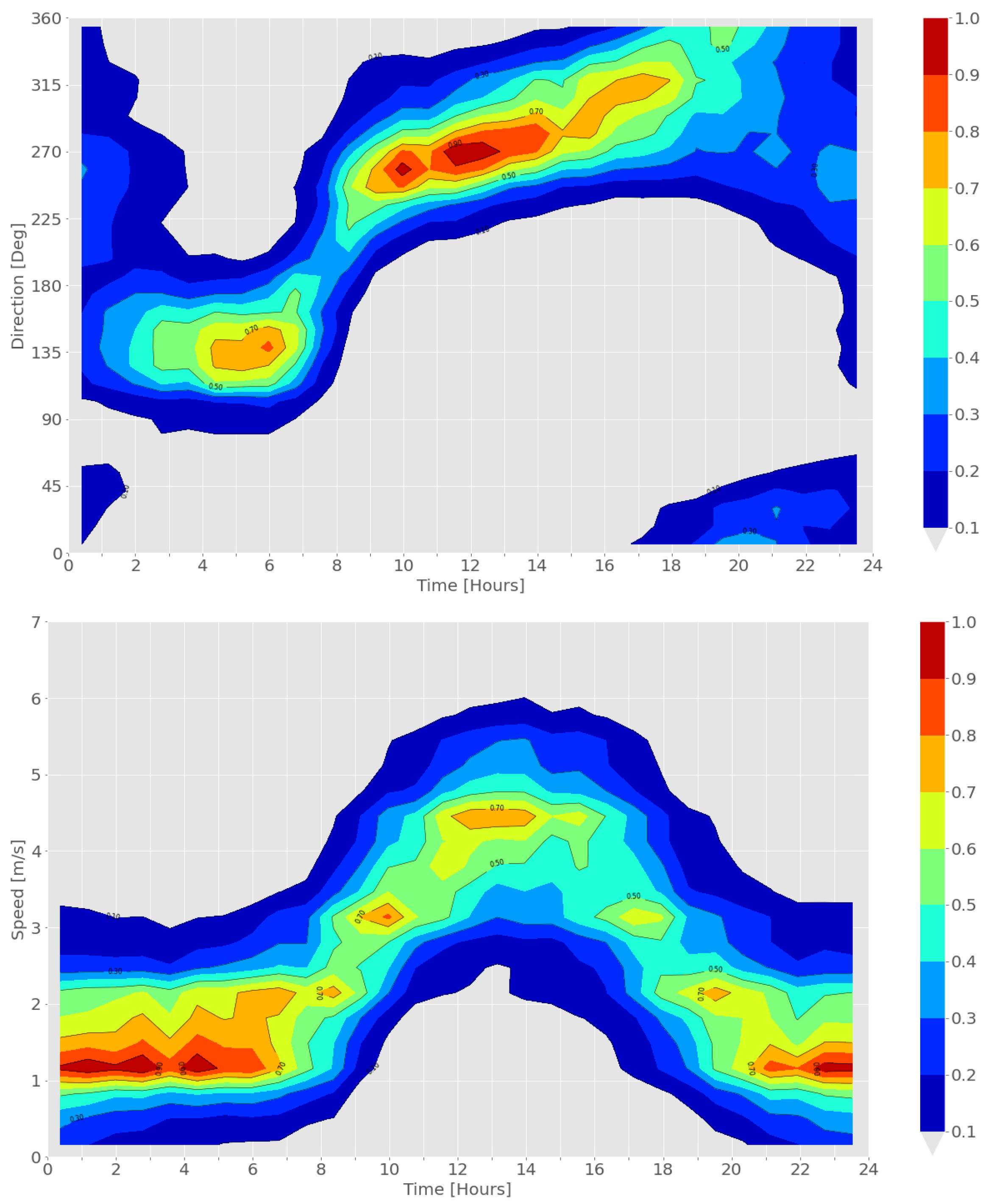
The diurnal time series of the wind speed and direction may change in time, from day to day, and in space, from one weather station to another. However, it is possible to identify climatological patterns in these time series, if each pair of time and wind vector component observation (either the direction or speed) is defined as a realization of a bivariate distribution. In this study, the time series from the four stations were grouped into two dimensional histograms, which were later plotted in a form of density contours. This resulted in a nonparametric visualization of the bivariate (time-speed or time-direction) distribution. Each contour represents a boundary in which a given percentile of the nonparametric bivariate distribution is contained.

3. Results and Discussion

To demonstrate the methodology described above, we chose to study the concentration profile at two points—the “Edgar Tower” (32 3 43 N × 34 47 19 E) which is located at the center of the Tel Aviv in the close proximity of main traffic routes and a junction of two main streets in city of Ramat-Gan (32 5 24 N × 34 49 20 E), a suburban of Tel-aviv. For each point the total concentration accumulates between 08:00–09:00 and 18:00–19:00 was calculated, which represents the expected pollution at rush hour in the summer. As will be discussed later the POI’s differ by the distribution of the pollutant sources in their close proximity. While the first point is located in the center of a very crowded routes, the influence on the second point comes mainly from more distanced places. In this study we shell examine the effect of this difference on the concentration profile. Specification of the method described before for these cases will be given here.

3.1. Climatology

The wind speed at Tel Aviv Metropolitan Area exhibit a clear diurnal regime. The wind speed is weak during the night. It increases during the morning, beginning around 0700 h, and begins to decrease in the afternoon, around 1700 h. During the periods of time where the wind is weak, its distribution is centered around 1–1.5 m/s. The wind speed reaches a single maximum between 1200 h to 1400 h, where the distribution is centered around 4.5 m/s. Along the day, the width of the distribution is rather constant, 3 m/s (Top panel of Figure 2). This wind speed diurnal regime was identified in other locations along the Israeli Mediterranean coast, both farther north in the Haifa bay area as well as farther south, in the southern coastal plain of Israel [78,79]. As Tel Aviv Metropolitan Area, the Haifa bay area and the southern coastal plain are all regions that are adjacent to the Mediterranean Sea, it can be deduced that they are all affected by the land-sea temperature difference. This phenomenon is closely related to the sea breeze [79].
Contrary to the rather simple behavior of the wind speed, of a single maximum around noon-time, the wind direction in Tel Aviv Metropolitan Area exhibits a more intricate behavior. Beginning around 0900 h up until 2100 h, the wind regime is composed of winds from the west, due to the Mediterranean sea-breeze combined with a Persian trough. The center of the distribution veers from the WSW (247 ) to N (0 ). As this period is influenced by the sea breeze, it can be referred as the daytime breeze period. During the night time, from 0100 h to 0700 h, a regime of non-veering directions centered around the SW (135 ), which is a combination of Katabatic land winds sliding from the Judea mountains and land breeze. This period can be referred to as the nighttime breeze period. Between these two regime, transition periods occur, in proximity to sunrise and sunset. Compared to the sunset transition period, the sunrise transition period is considerably shorter (lower panel of Figure 2). The change of direction during these periods does not follow a constant pattern. Sometimes, the wind direction can either turn clockwise or anti-clockwise [80].

3.2. Morphology

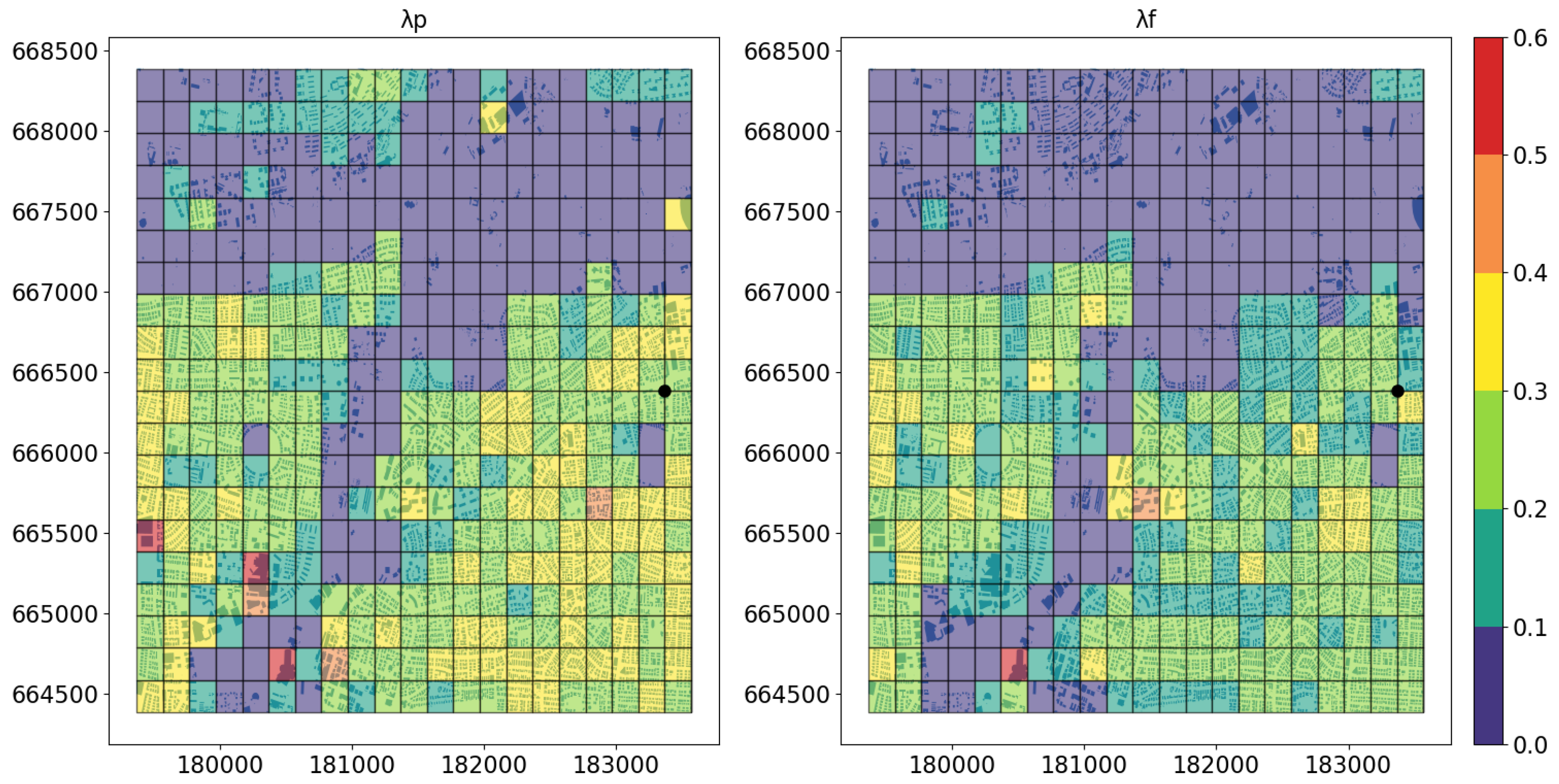
After the wind direction had been determined, the morphological parameters were calculated according to the procedure described before. In Figure 3 (left) map of λ f and λ p are given for every 200 m × 200 m cell in the relevant area for third case in Table 1. Since most of the impact on the dispersion comes from the close surrounding of the source position, the morphological parameters for every simulation was taken as the values of these parameters at the source position. It should be noted that we focus here on the buildings morphological parameters, while the effect of vegetation is neglected. This can be justified as in Tel Aviv the urban vegetation density is similar to the city of Haifa were we did validate our model with only the buildings used as morphological data [30].

3.3. Analyzed Cases

By taking the maximal value of the speed and direction distribution at every integration hour, we get full specification of the 4 cases analyzed in this study, summarized in Table 2. It should be noted that the morning scenarios (cases 1, 3) occur during the sunrise transition period, while the evening scenarios (cases 2, 4) occur during the daytime time breeze regime. We assume that since at these hours the heat fluxes are low enough (due to small angle of the sun to earth surface), ether near neutral or very weak convective conditions prevail (i.e., in terms of MOST stability parameter: | ζ | 1 ).
As described before, the total pollutant concentration is accumulated over 1 h window [ T i , T N ] from all sources emitted before the end of this window. In addition, the emitting time is divided into 1 h time intervals, such that t N = T f , t N 1 = T i . Assuming that the wind is approximately stationary for a certain case, designated by v, and we are interested in the concentration collected at point r from source at r . Most of the particles expected to reach the detector after approximately τ = | r r v | + δ , where δ is some width taken to guarantee that almost all relevant particles had been included. In principle all particles spread before t N 1 τ will not arrive to the detector before the integration window starts. If τ < 1 hr this implies that the only two previous time intervals in the summation of Equation (11) will contributes to the total concentration.
Note that the wind direction for the relevant rush hour cases comes from the west (240–300 deg), so the relevant sources are bound by the coast line which is typically no longer then 4 km distanced from the POI. Hence, for wind speed of v = 2 − 3 m/s this implies that the condition mentioned before is valid, i.e., only two terms has to be included in the evaluation of the integral. Therefore the concentration collected over the time window [ T i , T f ] from the k’th cell located at V k can be evaluated by the following expression:
D k = Q k , N 1 T i T f T i T f V k P f ( r , t | r , t ) d r d t d t + Q k , N 2 T i T f T i 1 T i V k P f ( r , t | r , t ) d r d t d t
The last expression can be understood as follows: the first term represents all the pollutant spread and collected at the current time interval. The second term add the contribution of pollutant from the previous time interval to the integration window. Thus, two LSM operations has to be performed in order to calculate the integral pollutant concentration at the POI from a single area source.

3.4. Profile Calculation

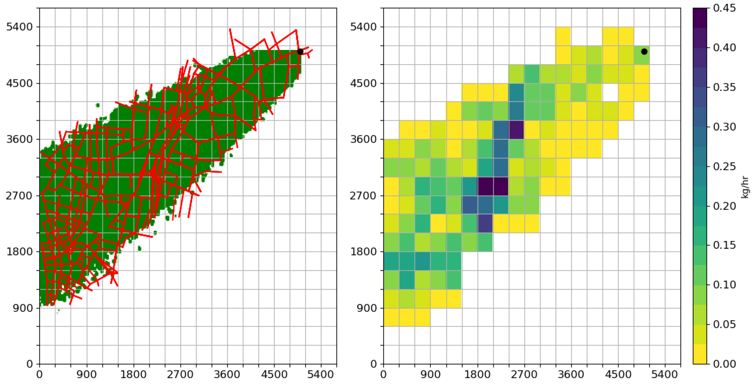
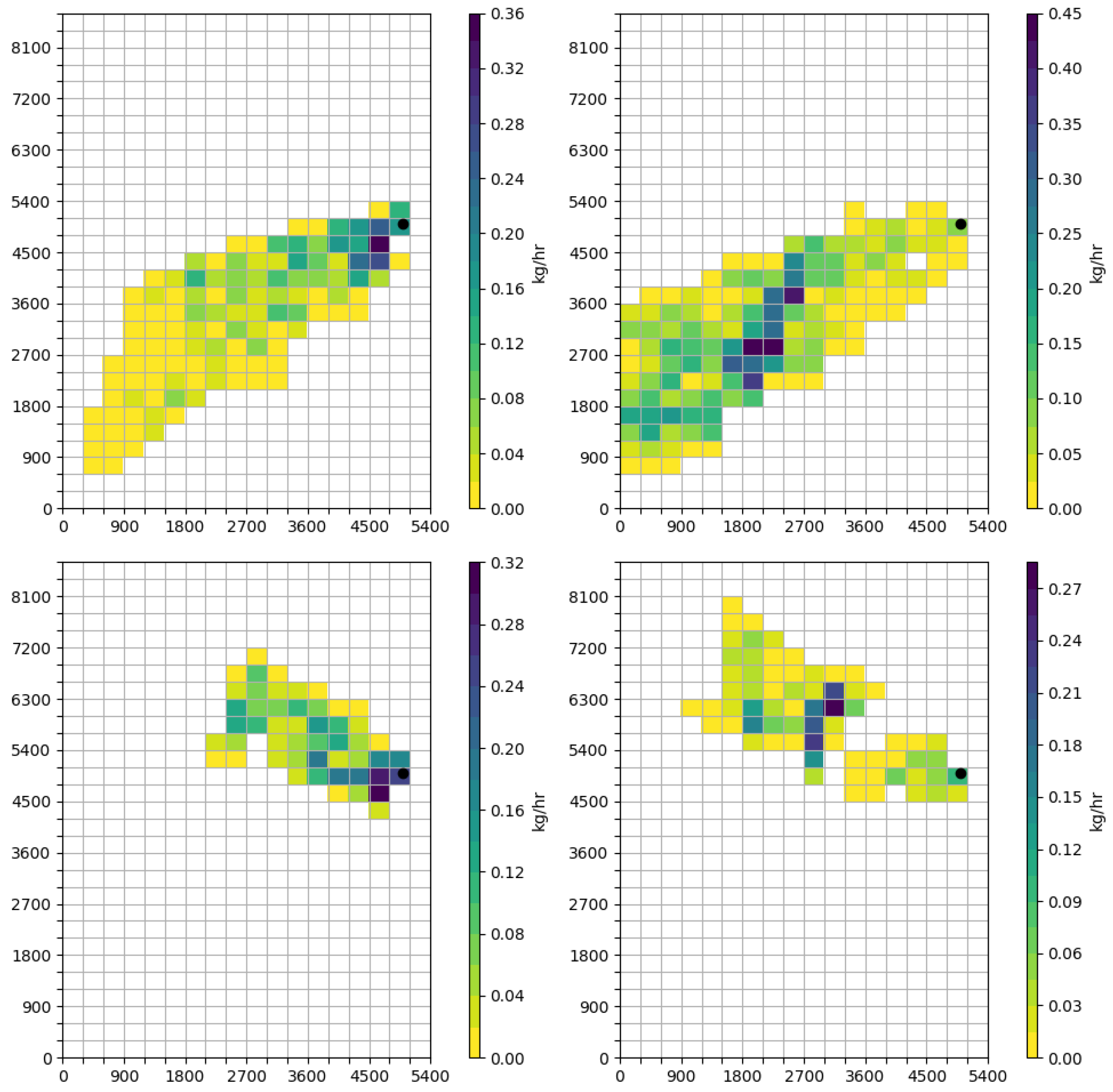
As mentioned before, footprint analysis was used to estimate the relevant part of space viewed by the POI. The threshold concentration was taken as 0.1 of the typical background concentration, which is about 21 μ g/m 3 [81]. A detailed demonstration of this analysis for the third case can be seen in Figure 4 (For clarity from here on, the coordinate system of all Figures was shifted such that the POI is always centered at (5000, 5000)). In the left panel the footprint calculated by Equation (15) starting from the POI, is shown in green and all the routes contained within in red. In the right panel a map of the area sources, calculated by summing all the corresponding routes in each cell, is shown. These sources are the basis for the rest of the methodology, as from each one of them two LSM simulation were performed which corresponds to the two terms in Equation (16). A corresponding bLSM-based footprint screening step had been performed for all four cases and the source map for each POI (columns) and wind regime (rows) is shown in Figure 5.
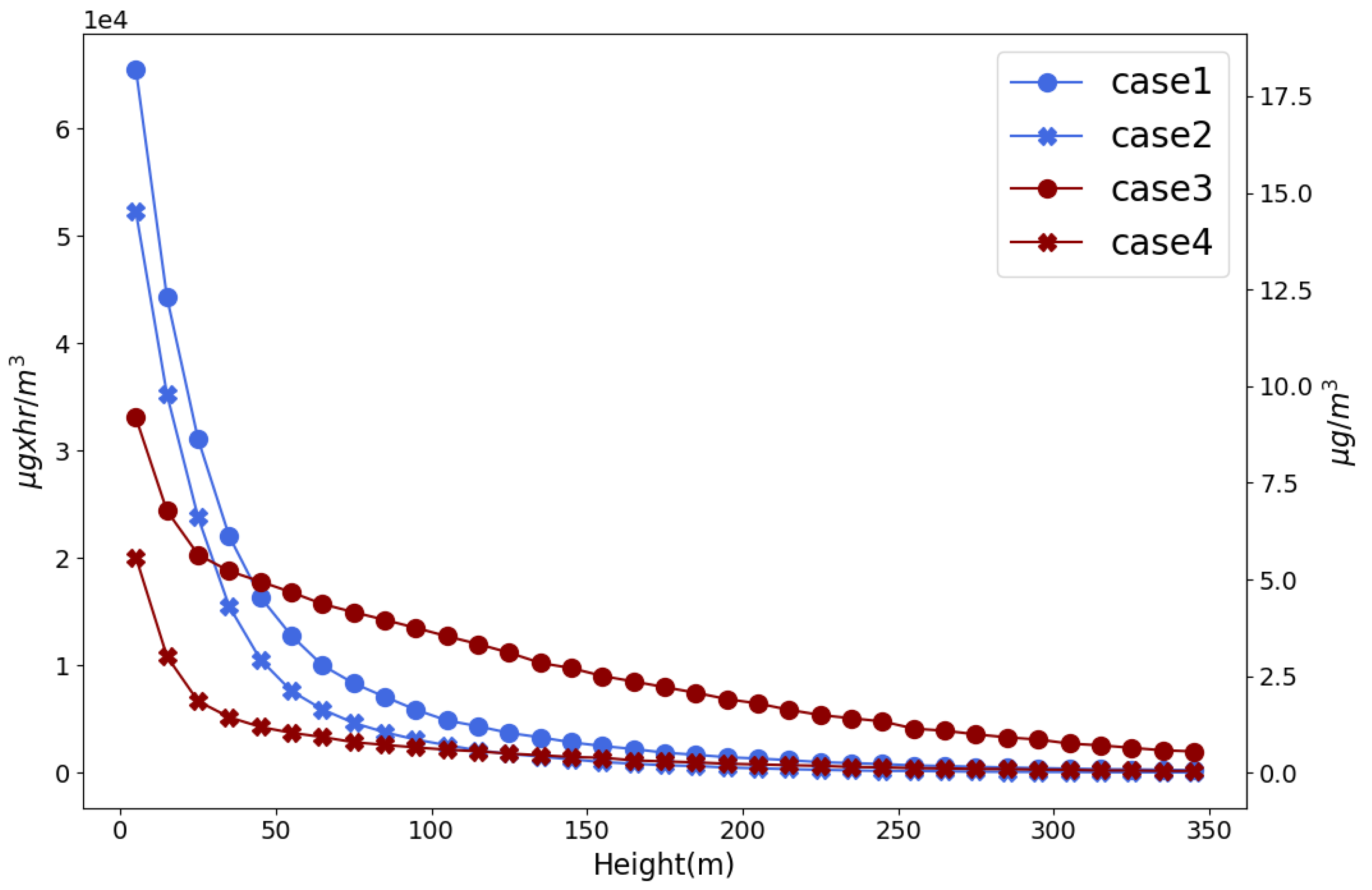
In Figure 6 the concentration profile for the four cases is shown. Both profiles for the first POI reviles a similar behavior, characterized by about 5–6 × 10 4 μ g × h/m 3 at the ground floor, which vanishes after approximately 200 m. The value at ground floor, after dividing by the time of integration, is about 16 μ g/m 3 which is very similar to the (yearly averaged) instantaneous concentration measured in Tel Aviv Metropolitan Area which is 21 μ g/m 3 [81].
The profiles of the second point are more diverse. The profile of the fourth case starts at lower concentration at ground level and decays fast with height. This can be explained by the gap of pollutant emissions in the area source map for this case (see in the lower right panel of Figure 5) which is the results of massive urban green space (“Hyarkon Park”). In contrast the profile of the third case starts from higher concentration and decays much slower then all other cases. Surprisingly, from height of 50 m the pollutant concentration at this point, located in a suburban of Tel Aviv is higher then the first point located in the center of Tel Aviv.
The difference in the profile shapes can be understood by comparing the area sources maps for each case, as discussed in Figure 5. Note that for first two cases, the cells with high emissions are located in the close proximity of the POI, while in the third case they are distanced about 3 km downwind from the point. This has a major effect on the concentration profile, since at lower heights most of the contributions to the concentration at certain point comes from its close proximity, while as the height increases more distanced cells dominates. Therefore for the first two cases the close surrounding dominants the profile, while at the third case the highly emission cells gives a significant contribution to higher heights.
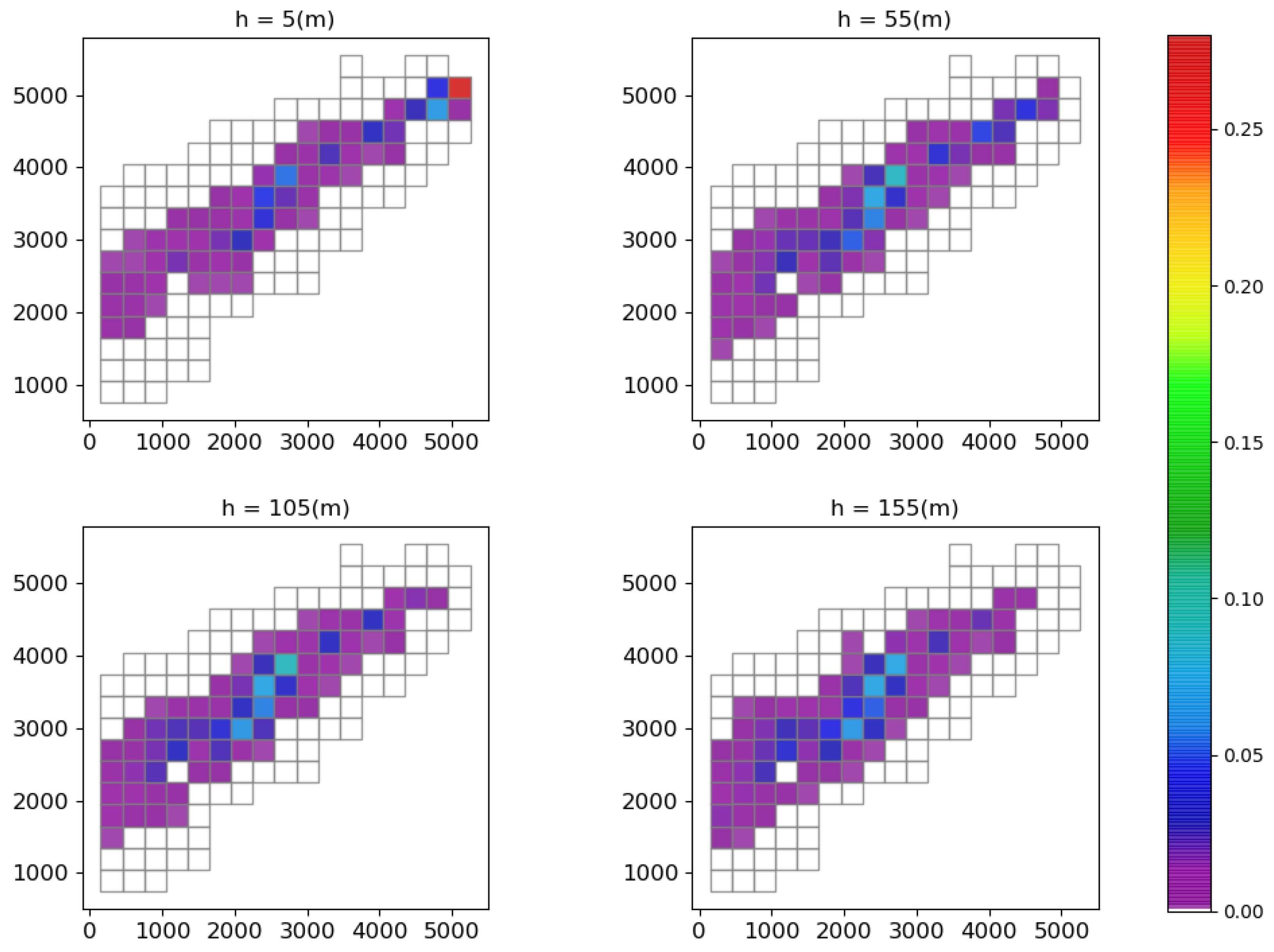
Quantification of this claim can be shown in Figure 7, where the relative contribution of each cell to the total calculate concentration at different heights (5, 55, 105, and 155 m) is shown for third case. At 5 m, about 40% of the concentration comes from the close surrounding, which is characterized by relatively low emissions so the total concentration is small. In contrast, at 105 m the contributions to the calculated concentration comes from a much wider regime, reaching its maximal value approximately at the maximal emitting cell. A similar picture emerges at 155 m which explains the slow decay shown in Figure 6.
An important emphasis of the current study is the attempt to reduce the computational effort required for the profile calculation. Two steps had been taken to achieve this goal: applying footprint analysis to identify the relevant part of space and merging the routes into area sources. The effect of these steps can be evaluated by comparing the number of area sources within the footprint ( N c e l l s ) to required LSM simulation from each traffic source without any screening ( N r o u t e s ). Some caution must be made however in order to make fair comparison, since the second number is given to some interpretation. Therefore we define a strip of 2 km along the wind direction for each case and calculated all the routes contained within downwind to the POI as reasonable evaluation for N r o u t e s . For example, for the third case, N c e l l s = 166 and N r o u t e s = 1600 so applying these steps can reduce the required computational effort by a order of magnitude. The efficiency of this procedure enables a relatively fast calculation of the profile, make it appealing for many uses.

4. Summary

In this study, an efficient methodology for evaluating the air pollution profile, induced by traffic sources, has been presented. This methodology relies on the ability of the LSM to calculate accurately the dispersion of the pollutant in a realistic complex scenario of urban canopy such as the Tel Aviv Metropolitan Area. This, however, requires the pre-determination of many input parameters such as details of multiple pollutant sources, meteorological, morphological and turbulent parameters. Although a single LSM simulation is known to be of relatively low computational effort, the simulation of urban traffic sources implies large number of sources and with it the computational cost rises. In this study we present an efficient methodology, using a footprint analysis based on bLSM, as well as on merging the traffic routs into area source cells (sub-areal sources). This methodology was implemented to calculate the concentration profiles for four exemplary cases in the Tel Aviv metropolitan area, differing by their location and wind regime. Different behaviors were shown for these cases, manifesting the unique combination of source structure, urban morphology, flow characteristics and the resultant dispersion pattern in each case. We show that as the height at the POI increases, the local close-by surrounding of the POI becomes less influential. We also demonstrated the effect of urban green space (park) on the reduction of concentration profile. This emphasises the importance of such an analysis for the impact on human exposure as well as for urban planning, and therefore the necessity of an efficient computational methodology, such as the one presented in this study.

Author Contributions

Conceptualization, E.F. and O.B.; Data curation, E.F., H.D.-S., Z.K. and O.B.; Formal analysis, E.F., H.D.-S. and O.B.; Funding acquisition, E.F.; Methodology, E.F. and O.B.; Project administration, E.F., Z.K. and O.B.; Resources, E.F., Z.K. and O.B.; Software, E.F., H.D.-S. and O.B.; Supervision, E.F., Z.K. and O.B.; Validation, E.F., H.D.-S. and O.B.; Visualization, E.F., H.D.-S. and O.B.; Writing—original draft, E.F., Z.K. and O.B.; Writing—review & editing, E.F., H.D.-S., Z.K. and O.B.; All authors have read and agreed to the published version of the manuscript.

Funding

This research was partially funded by the Israeli Ministry of Environmental Protection, grant number-190-1-1.

Institutional Review Board Statement

Non applicable.

Informed Consent Statement

Non applicable.

Data Availability Statement

The meteorological data used in this study was obtained from the ongoing monitoring networks of the IMS (Israel Meteorological Service) and the MoAg (Israel Ministry of Agriculture and Rural Development). The MoAg network includes data from weather stations owned by the MoAg as well as stations owned by other organisations and governmenral ministries. The IMS data is available at (https://ims.data.gov.il/ims/7, accessed on 8 February 2021). The MoAg data is available at (https://meteo.co.il/, accessed on 8 February 2021).

Acknowledgments

The authors wish to thank Ilan Levy from the Israeli Ministry of Environmental Protection for providing and discussing the details of the traffic pollution data.

Conflicts of Interest

The authors declare no conflict of interest.

References

  1. Meier-Girard, D.; Delgado-Eckert, E.; Schaffner, E.; Schindler, C.; Künzli, N.; Adam, M.; Pichot, V.; Kronenberg, F.; Imboden, M.; Frey, U.; et al. Association of long-term exposure to traffic-related PM10 with heart rate variability and heart rate dynamics in healthy subjects. Environ. Int. 2019, 125, 4429–4439. [Google Scholar] [CrossRef] [PubMed]
  2. Khreis, H.; Kelly, C.; Tate, J.; Parslow, R.; Lucas, K.; Nieuwenhuijsen, M. Exposure to traffic-related air pollution and risk of development of childhood asthma: A systematic review and meta-analysis. Environ. Int. 2017, 100, 1–31. [Google Scholar] [CrossRef] [Green Version]
  3. Eitan, O.; Barchana, M.; Dubnov, J.; Linn, S.; Carmel, Y.; Broday, D.M. Spatial analysis of air pollution and cancer incidence rates in Haifa Bay, Israel. Sci. Total Environ. 2010, 408, 4429–4439. [Google Scholar] [CrossRef] [PubMed]
  4. Yuval; Broday, D.M. High-resolution spatial patterns of long-term mean concentrations of air pollutants in Haifa Bay area. Atmos. Environ. 2006, 40, 3653–3664. [Google Scholar] [CrossRef]
  5. Sasaki, K.; Sakamoto, K. Vertical differences in the composition of PM10 and PM2.5 in the urban atmosphere of Osaka, Japanl. Atmos. Environ. 2005, 39, 7240–7250. [Google Scholar] [CrossRef]
  6. Zhang, Y.F.; Xu, H.; Tian, Y.Z.; Shi, G.L.; Zeng, F.; Wu, J.H.; Zhang, X.Y.; Li, X.; Zhu, T.; Feng, Y.C. The study on vertical variability of PM10 and the possible sources on a 220 m tower, in Tianjin, China. Atmos. Environ. 2011, 45, 6133–6140. [Google Scholar] [CrossRef]
  7. Chan, C.Y.; Xu, X.D.; Li, Y.S.; Wong, K.H.; Ding, G.A.; Chan, L.Y.; Cheng, X.H. Characteristics of vertical profiles and sources of PM2.5, PM10 and carbonaceous species in Beijing. Atmos. Environ. 2005, 39, 5113–5124. [Google Scholar] [CrossRef]
  8. Pateraki, S.; Manousakas, M.; Bairachtari, K.; Kantarelou, V.; Eleftheriadis, K.; Vasilakos, C.; Assimakopoulos, V.D.; Maggos, T. The traffic signature on the vertical PM profile: Environmental and health risks within an urban roadside environment. Sci. Total Environ. 2019, 646, 448–459. [Google Scholar] [CrossRef]
  9. Roth, M. Review of atmospheric turbulence over cities. Q. J. R. Meteorol. Soc. 2000, 126, 941–990. [Google Scholar] [CrossRef]
  10. Belcher, S.E.; Finnigan, J.J.; Harman, I.N. Flows through forest canopies in complex terrain. Ecol. Appl. 2008, 18, 1436–1453. [Google Scholar] [CrossRef] [PubMed]
  11. Finnigan, J.J. Turbulence in plant canopies. Annu. Rev. Fluid Mech. 2000, 32, 519–571. [Google Scholar] [CrossRef]
  12. Finnigan, J.J.; Shaw, R.H.; Patton, E.G. Turbulence structure above a vegetation canopy. J. Fluid Mech. 2009, 637, 387. [Google Scholar] [CrossRef] [Green Version]
  13. Shnapp, R.; Bohbot-Raviv, Y.; Liberzon, A.; Fattal, E. Turbulence–Obstacle Interactions in the Lagrangian Framework: Applications for Stochastic Modeling in Canopy Flows. Phys. Rev. Fluids 2020, 5, 094601. [Google Scholar] [CrossRef]
  14. Grimmond, C.S.B.; Oke, T.R. Aerodynamic properties of urban areas derived from analysis of surface form. J. Appl. Meteorol. Climatol. 1999, 38, 1262–1292. [Google Scholar] [CrossRef]
  15. Belcher, S.E.; Jerram, N.; Hunt, J.C.R. Adjustment of a turbulent boundary layer to a canopy of roughness elements. J. Fluid Mech. 2003, 488, 369–398. [Google Scholar] [CrossRef] [Green Version]
  16. Wilson, D.J. Monin-Obukhov Functions for Standard Deviations of Velocity. Bound. Layer Meteorol. 2008, 129, 353–369. [Google Scholar] [CrossRef]
  17. Raupach, M.R.; Finnigan, J.J.; Brunet, Y. Coherent eddies and turbulence in vegetation canopies: The mixing-layer analogy. Bound. Layer Meteorol. 1996, 78, 351–382. [Google Scholar] [CrossRef]
  18. Neophytou, M.; Gowardhan, A.; Brown, M. An inter-comparison of three urban wind models using Oklahoma City Joint Urban 2003 wind field measurements. J. Wind Eng. Ind. Aerodyn. 2011, 99, 357–368. [Google Scholar] [CrossRef]
  19. Thomson, D.J. Criteria for the selection of stochastic models of particle trajectories in turbulent flows. J. Fluid Mech. 1987, 180, 529–556. [Google Scholar] [CrossRef]
  20. Wilson, D.J.; Sawford, B.L. Review of Lagrangian stochastic models for trajectories in the turbulent atmosphere. Bound. Layer Meteorol. 1996, 78, 191–210. [Google Scholar] [CrossRef]
  21. Gavze, E.; Fattal, E. A Semi-analytical Model for Short-Range Near-Ground Continuous Dispersion. Bound. Layer Meteorol. 2018, 169, 297–326. [Google Scholar] [CrossRef]
  22. Wilson, J.D. Turbulent transport within the plant canopy. Estim. Areal Evapotranspir. 1989, 177, 43–80. [Google Scholar]
  23. Hanna, S.R.; Brown, M.J.; Camelli, F.E.; Chan, S.T.; Coirier, W.J.; Hansen, O.R.; Huber, A.H.; Kim, S.; Reynolds, R.M. Detailed simulations of atmospheric flow and dispersion in downtown Manhattan: An applications of five computational fluid dynamics models. Bull. Am. Meteorol. Soc. 2006, 87, 1713–1726. [Google Scholar] [CrossRef] [Green Version]
  24. Wilson, D.J.; Yee, E.; Ek, N.; Amours, R. Lagrangian simulation of wind transport in the urban environment. Q. J. R. Meteorol. Soc. 2009, 1602, 1586–1602. [Google Scholar] [CrossRef]
  25. Wang, C.; Li, Q.; Wang, Z.H. Quantifying the impact of urban trees on passive pollutant dispersion using a coupled large-eddy simulation–Lagrangian stochastic model. Build. Environ. 2018, 145, 33–49. [Google Scholar] [CrossRef]
  26. Rockle, R. Bestimmung der Stomungsver-Haltnisse im Bereich Komplexer Bebauugsstruk-Turen. Ph.D. Thesis, Fachbereich Mechanik, der Technischen Hochschule Darmstadt, Darmstadt, Germany, 1990. [Google Scholar]
  27. Kaplan, H.; Dinar, N. A Lagrangian Dispersion Model for Calculating Concentrations Distribution Within a Built-up Domain. Atmos. Environ. 1996, 30, 4197–4207. [Google Scholar] [CrossRef]
  28. Pardyjak, E.R.; Brown, M.J. Fast response modeling of a two building urban street canyon. In Proceedings of the Fourth Symposium on the Urban Environment, American Meteorological Society, Atlanta, GA, USA, 20–24 May 2002; p. J1.4. [Google Scholar]
  29. Moussafir, J.; Oldrini, O.; Tinarelli, G.; Sontowski, J.; Catherine, M.D. A New Operational Approach to Deal with Dispersion Around Obstacles: The Mss (Micro Swift Spray) Software Suite. In Proceedings of the 9th International Conference on Harmonisation within Atmospheric Dispersion Modelling for Regulatory Purposes, Garmisch-Partenkirchen, Germany, 1–4 June 2004; Volume 5.26. [Google Scholar]
  30. Fattal, E. A Non-Homogeneous Non-Gaussian Lagrangian-Stochastic Model for Pollutant Dispersion in Complex Terrain, and Its Comparison to Haifa 2009 Tracer Campaign (in Hebrew); 2014/56/53/5614; Israel Institute for Biological Research: Ness-Ziona, Israel, 2014.
  31. Coceal, O.; Belcher, S.E. Mean winds through an inhomogeneous urban canopy. Bound. Layer Meteorol. 2005, 115, 47–68. [Google Scholar] [CrossRef]
  32. Finnigan, J. The footprint concept in complex terrain. Agric. For. Meteorol. 2004, 127, 117–129. [Google Scholar] [CrossRef]
  33. Wang, C.; Wang, Z.H.; Yang, J.; Li, Q. A Backward-Lagrangian-Stochastic Footprint Model for the Urban Environment. Bound. Layer Meteorol. 2018, 168, 59–80. [Google Scholar] [CrossRef]
  34. Fattal, E.; Gavze, E. Lagrangian-Stochastic Modeling of Pollutant Dispersion within the Urban Boundary-Layer over Complex Terrain-Israel, Haifa Campaign 2009. In Proceedings of the 2014 American Geophysical Union (AGU) Fall Meeting, San Francisco, CA, USA, 15–19 December 2014. [Google Scholar] [CrossRef]
  35. Fattal, E.; Buchman, O.; Gavze, E. A Lagrangian Stochastic Model for Urban Area over Complex Terrain-Comparison with Haifa Campaigns. In Proceedings of the 23rd Symposium on Boundary Layers and Turbulence, Oklahoma City, OK, USA, 11–15 June 2018. [Google Scholar]
  36. Obukhov, A.M. Description of Turbulence in Terms of Lagrangian Variables. Adv. Geophys. 1959, 6, 113–116. [Google Scholar] [CrossRef]
  37. Pope, S.B. Turbulent Flows; Cambridge University Press: Cambridge, UK, 2000. [Google Scholar] [CrossRef]
  38. Flesch, T.K.; Wilson, J.D. A two-dimensional trajectory-simulation model for non-Gaussian, inhomogeneous turbulence within plant canopies. Bound. Layer Meteorol. 1992, 61, 349–374. [Google Scholar] [CrossRef]
  39. Weil, J.C. Linking a Lagrangian Particle Dispersion Model with Three-Dimensional Eulerian Wind Field Models. J. Appl. Meteorol. Climatol. 2008, 47, 2463–2467. [Google Scholar] [CrossRef]
  40. Gardiner, C.W. Handbook of Stochastic Methods for Physics, Chemistry and the Natural Sciences; Springer: Berlin, Germany, 1997. [Google Scholar]
  41. Dinar, N. Mass consistent models for wind distribution in complex terrain-Fast algorithms for three dimensional problems. Bound. Layer Meteorol. 1984, 30, 177–199. [Google Scholar] [CrossRef]
  42. Bohbot-Raviv, Y.; Shnapp, R.; Liberzon, A.; Babin, V.; Fattal, E. Turbulence statistics of canopy-flows using novel Lagrangian measurements within an environmental wind tunnel. In Proceedings of the Physmod 2017—International Workshop on Physical Modelling of Flow and Dispersion Phenomena, École Centrale de Nantes, France, 23–25 August 2017. [Google Scholar]
  43. Shnapp, R.; Shapira, E.; Peri, D.; Bohbot-Raviv, Y.; Fattal, E.; Liberzon, A. Extended 3D-PTV for direct measurements of Lagrangian statistics of canopy turbulence in a wind tunnel. Sci. Rep. 2019, 9, 7405. [Google Scholar] [CrossRef] [PubMed] [Green Version]
  44. Shnapp, R. On small-scale and large-scale intermittency of Lagrangian statistics in canopy flow. J. Fluid Mech. 2021, 913, R2. [Google Scholar] [CrossRef]
  45. Poggi, D.; Katul, G.G.; Cassiani, M. On the anomalous behavior of the Lagrangian structure function similarity constant inside dense canopies. Atmos. Environ. 2008, 42, 4212–4231. [Google Scholar] [CrossRef]
  46. Du, S. Universality of the Lagrangian Velocity Stracture Function Constant (C0) Across Different kinds of Turbulence. Bound. Layer Meteorol. 1997, 83, 207–219. [Google Scholar] [CrossRef]
  47. Rizza, U.; Degrazia, G.A.; Mangia, C.; Filho, E.P.M. Estimation of the Kolmogorov constant for the Lagrangian velocity spectrum and structure function under different PBL stability regimes generated by LES. Phys. A Stat. Mech. Its Appl. 2010, 389, 4009–4017. [Google Scholar] [CrossRef]
  48. Christen, A.; Vogt, R.; Rotach, M.W. Profile measurements of selected turbulence parameters over different urban surfaces. In Proceedings of the 4th International Conference on Urban Air Quality, Prague, Czech Republic, 25–28 March 2003; pp. 408–411. [Google Scholar]
  49. Wilson, D.J.; Flesch, T.K. Trajectory curvature as a selection criterion for valid Lagrangian stochastic dispersion models. Bound. Layer Meteorol. 1997, 84, 411–425. [Google Scholar] [CrossRef]
  50. Sawford, B.L. Rotation of trajectories in lagrangian stochastic models of turbulent dispersion. Bound. Layer Meteorol. 1999, 93, 411–424. [Google Scholar] [CrossRef]
  51. Brouwers, J.J.H. Statistical description of turbulent dispersion. Phys. Rev. E 2012, 86, 066309. [Google Scholar] [CrossRef] [PubMed] [Green Version]
  52. Gloster, J.; Sellers, R.; Webster, H.; Valarcher, J.F. Assessing the risk of airborne spread of foot-and-mouth disease: A case study. Weather 2006, 61, 137–142. [Google Scholar] [CrossRef]
  53. Mayer, D.; Reiczigel, J.; Rubel, F. A Lagrangian particle model to predict the airborne spread of foot-and-mouth disease virus. Atmos. Environ. 2008, 42, 466–479. [Google Scholar] [CrossRef]
  54. Garner, M.G.; Hess, G.D.; Yang, X. An integrated modelling approach to assess the risk of wind-borne spread of foot-and-mouth disease virus from infected premises. Environ. Model. Assess. 2006, 11, 195–207. [Google Scholar] [CrossRef]
  55. Klausner, Z.; Klement, E.; Fattal, E. Modeling long distance dispersal of airborne foot-and-mouth disease virus as a polydisperse aerosol—Application to the emergence of a new strain from Egypt to Israel. Atmos. Environ. 2015, 122, 332–342. [Google Scholar] [CrossRef]
  56. Shi, J.P.; Mark, D.; Harrison, R.M. Characterization of particles from a current technology heavy-duty diesel engine. Environ. Sci. Technol. 2000, 34, 748–755. [Google Scholar] [CrossRef]
  57. Csanady, G.T. Turbulent Diffusion of Heavy Particles in the Atmosphere; D. Reidel Publishing: Dordrecht, The Netherlands, 1963. [Google Scholar] [CrossRef]
  58. Hanna, S.R.; Britter, R.E. Wind Flow and Vapor Cloud Dispersion at Industrial and Urban Sites; John Wiley & Sons, Inc.: Hoboken, NJ, USA, 2002. [Google Scholar] [CrossRef]
  59. Stull, R.B. An Introduction to Boundary Layer Meteorology, 1st ed.; Kluwer: Dordrecht, The Netherlands, 1988. [Google Scholar] [CrossRef]
  60. Raupach, M.R.; Shaw, R.H. Averaging procedures for flow canopies. Bound. Layer Meteorol. 1982, 22, 79–90. [Google Scholar] [CrossRef]
  61. Coceal, O.; Belcher, S.E. A canopy model of mean winds through urban areas. Q. J. R. Meteorol. Soc. 2004, 130, 1349–1372. [Google Scholar] [CrossRef] [Green Version]
  62. Britter, R.E.; Hanna, S.R. Flow and dispersion in urban areas. Annu. Rev. Fluid Mech. 2003, 35, 469–496. [Google Scholar] [CrossRef]
  63. Inoue, E. On the turbulent structure of airflow within crop canopies. J. Meteorol. Soc. Jpn. 1963, 41, 317–326. [Google Scholar] [CrossRef] [Green Version]
  64. Finnigan, J.; Harman, I.; Ross, A.; Belcher, S.E. First-order turbulence closure for modelling complex canopy flows. Q. J. R. Meteorol. Soc. 2015, 141, 2907–2916. [Google Scholar] [CrossRef] [Green Version]
  65. Harman, I.N.; Finnigan, J.J. A simple unified theory for flow in the canopy and roughness sublayer. Bound. Layer Meteorol. 2007, 123, 339–363. [Google Scholar] [CrossRef]
  66. Hicks, B.B.; Pendergrass, W.R.; Vogel, C.a.; Keener, R.N.; Leyton, S.M. On the Micrometeorology of the Southern Great Plains 1: Legacy Relationships Revisited. Bound. Layer Meteorol. 2014, 151, 389–405. [Google Scholar] [CrossRef]
  67. Hanna, S.R. Applications in air pollution modelling. In Atmospheric Turbulence and Air Pollution Modelling; Nieuwstadt, F.T.M., van Dop, H., Eds.; D. Reidel Publishing: Dordrecht, The Netherlands, 1982; p. 275. [Google Scholar] [CrossRef]
  68. Kastner-Klein, P.; Rotach, M.W. Mean flow and turbulence characteristics in an urban roughness sublayer. Bound. Layer Meteorol. 2004, 111, 55–84. [Google Scholar] [CrossRef]
  69. Mortarini, L.; Ferrero, E.; Richiardone, R.; Falabino, S.; Anfossi, D.; Trini Castelli, S.; Carretto, E. Assessment of dispersion parameterizations through wind data measured by three sonic anemometers in a urban canopy. Adv. Sci. Res. 2009, 3, 91–98. [Google Scholar] [CrossRef] [Green Version]
  70. Flesch, T.K.; Wilson, J.D.; Yee, E. Backward-time Lagrangian stochastic dispersion models and their application to estimate gaseous emissions. J. Appl. Meteorol. 1995, 34, 1320–1332. [Google Scholar] [CrossRef] [Green Version]
  71. Buchman, O.; Fattal, E. A Method for Source Location Estimation Based on Backward Lagrangian Stochastic Model. 2019/56/37/5614; Israel Institute for Biological Research: Ness-Ziona, Israel, 2019.
  72. Buchman, O.; Fattal, E. Adaptive degenerate space method for source term estimation using a backward Lagrangian stochastic model. arXiv 2020, arXiv:2004.06526. [Google Scholar]
  73. Sawford, B.L. Lagrangian Statistical Simulation of Concentration Mean and Fluctuation Fields. J. Clim. Appl. Meteorol. 1985, 24, 1152–1166. [Google Scholar] [CrossRef]
  74. Israel Ministry of Environmental Protection. Israel Road Traffic Emissions Inventory for the Year 2019; Received by Authors Request; Israel Ministry of Environmental Protection: Tel-Aviv, Israel, 2019.
  75. Wilson, J.D.; Swaters, G.E. The source area influencing a measurement in the Planetary Boundary Layer: The “footprint” and the “distribution of contact distance”. Bound. Layer Meteorol. 1991, 55, 25–46. [Google Scholar] [CrossRef]
  76. Schmid, H.P. Source areas for scalars and scalar fluxes. Bound. Layer Meteorol. 1994, 67, 293–318. [Google Scholar] [CrossRef]
  77. Alpert, P.; Osetinsky, I.; Ziv, B.; Shafir, H. A new seasons definition based on classified daily synoptic systems: An example for the eastern Mediterranean. Int. J. Climatol. 2004, 24, 1013–1021. [Google Scholar] [CrossRef]
  78. Klausner, Z.; Ben-efraim, M.; Arav, Y.; Tas, E.; Fattal, E. The micrometeorology of the Haifa bay area and Mount Carmel–Summer flow regimes. Atmosphere 2021, 12, 354. [Google Scholar] [CrossRef]
  79. Goldreich, Y. The Climate of Israel: Observation, Research and Application; Springer: New York, NY, USA, 1998; ISBN 9781461352006. [Google Scholar]
  80. Klausner, Z.; Fattal, E. An objective and automatic method for identification of pattern changes in wind direction time series. Int. J. Climatol. 2011, 31, 783–790. [Google Scholar] [CrossRef]
  81. Background_ENV_DATA; Ministry of Environmental Protection, Air Quality Division: Tel-Aviv, Israel, 2014. Available online: https://www.gov.il/BlobFolder/policy/guidelines_conducting_environmental_survey_air_pollution_transportation/he/transportation_airpollutants_by_land_area.pdf (accessed on 22 February 2021).
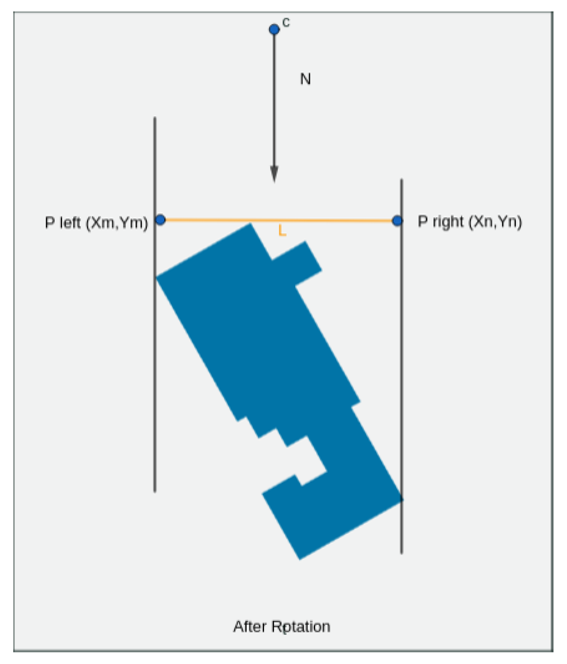
Figure 1. A demonstration of λ f calculation by searching the maximal distance between two vertices of the building.
Atmosphere 12 00580 g001
Figure 2. Nonparametric bivariate density of the climatological Tel Aviv summer wind diurnal distribution: upper: wind direction, lower: wind speed. The colored contours represent a given fraction of the distribution. All time points are in LST (UTC + 2).
Atmosphere 12 00580 g002
Figure 3. A map of all the buildings in the relevant part of Tel Aviv metropolitan area for the third case described in Table 2 is shown (black point represents the location of the POI in this case). The grid (200 m × 200 m) layer on top of this map, represents the average morphological parameters ( λ p (left) and λ f (right)) as calculated in Equation (6) (Israeli Traverse Mercator (EPSG 2039) is used for this figure; The 6-digit coordinates are expressed in meters).
Atmosphere 12 00580 g003
Figure 4. Left panel: the non-zero (footprint) part of the Backward dispersion map, starts from the second POI (case 3), is shown in green. This area represent all the relevant part of space which may contributes to the concentration at the POI (located at ( 5000 , 5000 ) in this map). All the relevant routes contained within are shown by red lines. Right panel: The area source map, constructed by summing all the routes within every cell.
Atmosphere 12 00580 g004
Figure 5. The area source map is shown for all four cases described in Table 2. In the left column the map for the first point (“Edgar tower”) for wind regime of 2 m/s in 240 direction (first row) and 3 m/s in 300 direction (second row). In the right column, the corresponding maps for the second POI (“Ben-Gurion junction”) is shown for both meteorological scenarios. In all cases the POI is located at (5000,5000) (shown by a black dot).
Atmosphere 12 00580 g005
Figure 6. The accumulate and instantaneous concentration profile (left and right vertical axis) induced by traffic sources for all cases described in Table 1 is shown.
Atmosphere 12 00580 g006
Figure 7. The relative contribution of different cells to the pollutant concentration at the second POI (case 3; located at ( 5000 , 5000 ) ) at four heights for third case is shown.
Atmosphere 12 00580 g007
Table 1. The stations analysed in this study. Stations owners and abbreviations: IMS (Israel Meteorological Service), MoAg (Israel Ministry of Agriculture and Rural Development), MoEP (Israel Ministry of Environemtnal Protection). These stations are a part of ongoing monitoring networks available online: IMS (https://ims.data.gov.il/ims/7 (accessed on 8 February 2021)), MoAg and EPA (https://meteo.co.il/ (accessed on 8 February 2021)).
Station NameLocationWind SensorElevation ASL [m]Owner
Bet Dagan32 0 26 N 34 48 50 EPropeller-vane anemometer31IMS
Tel Aviv Coast32 3 29 N 34 45 32 EPropeller-vane anemometer10IMS
Tel Aviv Kremenetski32 3 59 N 34 47 42 ECup anemometer + vane17MoAg
Tel Aviv university32 48 4 N 34 59 30 ECup anemometer + vane28MoEP
Table 2. The wind parameters of the the four cases analyzed in this work.
CasePoint T i T f Speed (m/s)Direction
1Edgar Tower08:0009:002240
2Edgar Tower18:0019:003300
3Ben Gurion st.08:0009:002240
4Ben Gurion st.18:0019:003300
Publisher’s Note: MDPI stays neutral with regard to jurisdictional claims in published maps and institutional affiliations.