Article

Surface and Tropospheric Response of North Atlantic Summer Climate from Paleoclimate Simulations of the Past Millennium

by
Maria Pyrina
1,2,*,
Eduardo Moreno-Chamarro
3,
Sebastian Wagner
1 and
Eduardo Zorita
1
1
Helmholtz-Zentrum Hereon, Institute of Coastal Systems, 21502 Geesthacht, Germany
2
ETH Zurich, Institute for Atmospheric and Climate Science, 8092 Zurich, Switzerland
3
Barcelona Supercomputing Center, 08034 Barcelona, Spain
*
Author to whom correspondence should be addressed.
Atmosphere 2021, 12(5), 568; https://doi.org/10.3390/atmos12050568
Submission received: 29 March 2021 / Revised: 21 April 2021 / Accepted: 25 April 2021 / Published: 28 April 2021
(This article belongs to the Special Issue Links between Solar Activity and Atmospheric Circulation)

Abstract

:
We investigate the effects of solar forcing on the North Atlantic (NA) summer climate, in climate simulations with Earth System Models (ESMs), over the preindustrial past millennium (AD 850–1849). We use one simulation and a four-member ensemble performed with the MPI-ESM-P and CESM-LME models, respectively, forced only by low-scaling variations in Total Solar Irradiance (TSI). We apply linear methods (correlation and regression) and composite analysis to estimate the NA surface and tropospheric climatic responses to decadal solar variability. Linear methods in the CESM ensemble indicate a weak summer response in sea-level pressure (SLP) and 500-hPa geopotential height to TSI, with decreased values over Greenland and increased values over the NA subtropics. Composite analysis indicates that, during high-TSI periods, SLP decreases over eastern Canada and the geopotential height at 500-hPa increases over the subtropical NA. The possible summer response of SSTs is overlapped by model internal variability. Therefore, for low-scaling TSI changes, state-of-the-art ESMs disagree on the NA surface climatic effect of solar forcing indicated by proxy-based studies during the preindustrial millennium. The analysis of control simulations indicates that, in all climatic variables studied, spurious patterns of apparent solar response may arise from the analysis of single model simulations.

1. Introduction

Changes in the climate system may be a result of internal climate variability or external influences that may be either anthropogenic or natural (i.e., orbital, solar, or volcanic forcing). The human influence on global temperature since the start of the industrial era (after AD 1850) has very likely exceeded the impact of natural forcings [1]. However, during the pre-industrial era, externally driven climate change at decadal-to-multidecadal time scales is considered to be forced primarily by variation in solar output and by volcanic eruptions [2,3,4]. In contrast to volcanic forcing, solar forcing may cause long-term (decadal mean) continental and regional climate changes that are greater than unforced (internal) variability [5].
The Sun’s climatic impact arises from changes in its total solar irradiance (TSI), spectral solar irradiance (SSI) and energetic particle precipitation (EPP) [6,7,8,9,10]. Recently, more efforts were placed on the representation of variations in SSI and EPP in climate model simulations, with new recommendations regarding the magnitude of SSI variations used to force state of the art global climate models. The SSI uncertainty and the possible impacts of the higher SSI variations are discussed extensively in Matthes et al. [11].
In the current study, we are interested in the climatic impact of TSI variations during the preindustrial last millennium (AD 850–1849), as TSI is used as proxy for identifying the effect of solar variability in paleoclimate proxy data. The effect of TSI changes on the climate of the past millennium was identified by early works in the context of the historical Maunder Minimum (AD 1675–1715) [12] and confirmed by more recent studies investigating climate changes during periods of solar maxima and minima [13,14,15,16]. In the early 2000s it was generally accepted that a long-term change in solar activity between the mean solar output during the Maunder Minimum (decline in solar activity) and the present-day climate, a period with presumably higher solar output, was about 0.3% [17]. However, the amplitude of these TSI changes was subsequently revised and reduced to a value of approximately 0.1% [18,19]. This new scaling was applied to the models participating in the 5th phase of the Coupled Model Intercomparison Project—CMIP5 [20,21]. Even though this change in the TSI scaling has implications for our understanding of the effects of changes in solar output on climate, a quantitative assessment of this effect has not yet been made.
We use simulations forced with the latest estimations of the solar amplitude and investigate how these TSI variations are reflected in the North Atlantic (NA) climate of model simulations in the preindustrial last millennium. We focus on the NA, where ocean-atmosphere interactions crucially affect the climate of North America and Europe [22,23,24], and on the summer season, as it is more relevant for comparison to studies using proxy data. Biological proxies, such as trees and bivalve shells, tend to reflect the growing season more strongly. The variability in their growth increment widths is related to environmental conditions and their growth is biased towards summer [25,26].
Investigating the Sun-climate relationship prior to industrial times is important for the comparison between climate models and proxy records and for disentangling anthropogenic climate change from natural variations [27]. Modeling and proxy-based studies have so far disagreed on the importance of TSI forcing on driving variations in global annual mean surface temperatures [28,29,30], but they agree on larger regional effects of TSI forcing [31,32,33]. Nevertheless, these effects might be too large to be attributed to direct solar heating, and positive feedbacks have been invoked [34], particularly in regions that usually are cloud covered [35,36,37]. Regarding the NA region, some authors have claimed the detection of influence of solar forcing in marine proxies over the past millennium for Sea Surface Temperatures (SSTs) in centennial and multi-decadal time scales [33,38,39].
Jiang et al. [38] used regression analysis and paleoclimate proxy data, and identified a positive correlation between SSTs and solar forcing for the region of the North Icelandic shelf. Further, these authors used composite analysis and found that surface temperatures north of Iceland increase for stronger solar forcing. In order to investigate whether such signals occur in model simulations, we make use of linear regression and composite analysis, and investigate the spatial climatic changes that are solely induced by changes in solar activity, during the summer seasons of AD 850–1849, over the North Atlantic. For this goal, we use solar-only forced CMIP5-type simulations available for the Max Planck Institute Earth System Model (MPI-ESM) and the Community Earth System Model (CESM). These simulations employ reduced long-term solar amplitudes, smaller than that used in simulations carried out one or two decades ago, and implement solar activity changes for different wavelength bands.
The use of only-solar forced simulations is important for having a clearer solar forcing signal, as solar forcing effects might be concealed by the larger effect of volcanic eruptions, for example, in periods when TSI minima coincided with volcanic eruptions during the last millennium. For this reason, the use of linear regression might not be appropriate for detecting the signal of solar forcing [40]. Moreover, the CESM output includes an ensemble of solar-only forced experiments. That is important in order to quantify the magnitude of model internal variability and the magnitude of the TSI effects on the modeled climate.
Other studies also used simulations with current estimations of long-term solar amplitudes and investigated the sun-climate relationship, but they investigated the winter season in the recent historical period and used fully forced experiments [41,42,43,44]. Our analysis focuses on summer season and the preindustrial period, therefore being more relevant to model-proxy comparisons. Moreover, the use of only-solar forced experiments during the preindustrial era automatically excludes possible influences from volcanic eruptions and anthropogenic forcing. Therefore, the investigation of the pure impact of changes in solar activity on the simulated climate is more robust. Another aspect of the paper is that our analysis includes different techniques for signal identification. Therefore, our results might help to disentangle potential solar-only induced changes from those of the fully forced runs, focusing spatially on the effect of model internal variability.

2. Materials and Methods

2.1. Model Simulations

2.1.1. MPI-ESM-P

We use two comprehensive Earth System Models (ESMs) participating in CMIP5 (https://pcmdi.llnl.gov/mips/cmip5/ (accessed on 30 October 2019). The first model is the MPI-ESM for paleo-applications (MPI-ESM-P) [45]. This configuration is identical to MPI-ESM-LR with two exceptions: the dynamical vegetation module is not active, so that land use changes can be prescribed, and the orbital parameters are prescribed by a table providing annual values for eccentricity, obliquity, and perihelion [46].
The atmosphere has a T63/1.9° horizontal resolution and 47 hybrid sigma pressure levels (ECHAM; [47]). The ocean grid is curvilinear bipolar with an effective 1.5° resolution (near the equator) and 40 z-levels (MPIOM; [48]). The atmospheric grid extends to 0.01 hPa in the vertical domain, where the center of the topmost level in the upper mesosphere is set. This vertical extension of the atmospheric grid includes for the first time a better resolved stratosphere in CMIP simulations for MPI-M [49]. The solar spectrum is split into 14 spectral bands and temporal variations of solar irradiance depend on the wavelength. Here the relative variations among spectral bands are the result of a physically reasonable estimation, since the information provided by the ice-core records cannot differentiate between spectral bands [50]. The monthly average ozone concentrations for the period AD 850–1849 are also prescribed and were calculated using the AD 1850–1860 monthly climatology of ozone concentrations from the AC&C/SPARC Ozone Database as a basis. The ozone dependency on solar irradiance is represented through regression coefficients between historical ozone concentrations and the annual 180.5 nm solar flux [45].
We use a single simulation of the MPI-ESM-P model, the solar-only forced simulation MPI-R1. For solar radiation, the Vieira et al. [18] total solar irradiance reconstruction over the Holocene is employed with a TSI scaling of 0.1% from the 17th century Maunder Minimum to present [51]. Well mixed-greenhouse gases (CO2, CH4, N2O) and orbital parameters are annually varying [46].

2.1.2. CESM-LME

The second ESM used is the Community Earth System Model-Last Millennium Ensemble (CESM-LME; [52]). The CESM-LME employs the CESM-Community Atmosphere Model version 5 (CESM1-CAM5; [53]) with a difference in the resolution of its individual model components. The ocean component of CESM-LME has a 1º horizontal resolution, while the atmospheric component at 2° horizontal resolution extends from the surface to the middle stratosphere (~40 km) [54].
Radiative fluxes and heating rates in CAM5 are calculated using the Rapid Radiative Transfer Method for GCMs (RRTMG) [55], which separates the short-wave spectrum into 14 bands extending from 0.2 μm to 12.2593 μm. The TSI value is scaled in each spectral band through a specification of a time-varying solar spectral irradiance [56]. To provide fluxes at the top of the atmosphere, RRTMG uses an additional layer above the CAM5 model top in both the longwave and shortwave. This extra layer is specified by replicating the composition of the highest CAM5 layer into a layer that extends from the top of the model to 10−4 hPa. The radiation parameterization requires monthly mean ozone volume mixing ratios to be specified as a function of the latitude grid, vertical pressure levels, and time. The ozone path lengths are evaluated from the mixing–ratio data derived by Chervin [57] from analysis of Dütsch [58].
The CESM-LME solar-only experiments are forced with the same annually varying well mixed-greenhouse gases and orbital parameters as the MPI-ESM-P simulation [46], following the PMIP3 protocol. The CESM-LME uses the [18] total solar irradiance reconstruction over the Holocene to produce a four member solar-only forced ensemble over the period AD 850–2005. The only difference among its four ensemble members is the application of small random differences (order of 10–14 °C) in the air temperature field at the start of each ensemble member. Both the CESM-LME and the MPI-ESM-P simulations are analyzed for the preindustrial period AD 850–1849. For better comparison, the original model output was post-processed and re-gridded to a regular grid (1° × 1° degree horizontal resolution). In Table 1, details on the models and experiments used in this study are given.

2.2. Methods

To identify the effects of TSI forcing on the NA climate, we used three methods. The first method, Pearson Correlation, and the second method, Linear Regression, are linear parametric techniques that identify the linear dependence between variables. Both of these methods take into account the full preindustrial period, AD 850–1849. This analysis is performed for decadal low-pass filtered series, motivated by the multi-decadal surface response found in proxy data [38,39]. The decadal filtered series were obtained by filtering the climatic parameters and the TSI series in the spectral domain (cut off frequency = 1/11) using a low-pass filtering technique [59]. The low-pass filter applied isolates the signals with a frequency lower than the selected cutoff frequency. Therefore, variability is suppressed for time scales shorter than 11 years. Moreover, for the correlation analysis we also consider possible temporal lags in the solar-climate relationship.
The third method used is Composite Analysis, focusing on the effect of prominent TSI periods with high and low TSI values. Periods with high TSI are defined as those with positive TSI anomalies exceeding the +2.2 standard deviation, whereas periods with low TSI are defined as those with negative TSI anomalies lower than the −1.4 standard deviation (Figure 1a). These asymmetric requirements were set in order to have approximately the same amount of selected cases with positive (25 cases) and negative (20 cases) extreme TSI values, as the TSI distribution resembles a positively skewed non-Gaussian distribution (Figure 1b). It must be noted that such analysis does not account for lagged responses in the climate due to TSI changes.
We focus on the spatial climatic response pattern of the North Atlantic Ocean due to TSI changes during summer (June-August), including changes in atmospheric circulation. The geographical domain is between 80° W–30° E and 21° N–75° N. For all methods used and variables, the model data have been detrended prior to the analysis. Moreover, the TSI data have been detrended prior to the analysis. The reason is to avoid the identification of spurious relationships caused by possibly existing, but physically unrelated, trends in the data [60].
The statistical significance of the results obtained by these methods is tested with two approaches. One approach is the standard two-sided Student’s t-test. This test is applied in the linear methods to estimate the significance of the regression and correlation parameters. To account for the high degree of autocorrelation in the low-pass filtered series, we use a random-phase bootstrap method. This method preserves the spectrum and autocorrelation of the original time series, but the surrogate time series have a random time evolution [61,62]. A t-test is also applied in the results obtained by Composite Analysis to test the mean difference between the high-solar and low-solar samples. Because of the small sample size, the confidence intervals are estimated using a bootstrapping technique with replacement. We select two random subsets from the original time series with lengths equal to the original composite subsamples. A distribution of the differences is then constructed by repeating this procedure 1000 times.
Our null hypothesis H0 is that there is no effect of solar forcing on climate, i.e., that the regression and correlation parameters are zero and that there is no mean difference between the populations selected from years with high and low solar activity. If the null hypothesis is rejected at the significance alpha level α = 0.05, then we can reject the null hypothesis, and interpret that there is an effect of solar output on climate, with a 5% risk. However, statistical significance does not necessarily imply physical relevance. Especially for the linear methods, we use a large pool of samples (n = 1000) and the sample size is important for the estimation of the nominal level of statistical significance. As consequence, very large sample sizes will ultimately lead to the phenomenon that even very small physical quantities reach the statistical significance threshold for the alpha level under consideration.
The second approach we use to test the statistical significance of our results, regarding the possibly emerging signals of solar impact on climate, is the analysis of Preindustrial Control (PiControl) simulations conducted with the same ESMs. These control runs are conducted with the same models, but with constant external forcing (with the exception of a constant annual cycle of solar insolation). Any signal of solar impact on climate emerging in the control simulations, using the very same methods as for forced simulations, is due to random sampling and to the autocorrelation structure of the climate variables. Its amplitude yields a benchmark that needs to be surpassed by the solar-climate signals that are statistically identified in the forced simulations.

3. Results

Using the methodologies described before, we investigate the surface and tropospheric response to solar forcing over the North Atlantic during summer. Previous studies, mostly investigating the winter season, hypothesized that the simulated changes in solar forcing are integrated into the lower troposphere and therefore might affect both directly and indirectly the surface climate. The analysis is performed for decadal time scales using correlation and regression analysis. As suggested by [44], the use of the composite method avoids data filtering. Therefore, the results of the composite method do not take into account decadal time scales.

3.1. Linear Methods

The TSI time series is correlated and regressed to the oceanic and atmospheric variables for the period AD 850–1849. The Pearson correlation coefficients of TSI with sea surface temperature (SST), sea level pressure (SLP) and geopotential height at 500 hPa (geo500) are shown in Figure 2a–f, respectively. For the regression analysis, the TSI anomalies are standardized and subsequently regressed over the North Atlantic (NA) atmospheric and oceanic variables (Figure 3). Therefore, the regression results represent changes of the climatic variables that correspond to changes of one standard deviation (SD) of TSI. The results are given in the first row for the MPI-ESM single simulation and in the second row for the CESM ensemble mean.
On decadal time scales, the TSI signal is generally weakly correlated (r < ±0.2) with SST and SLP in both models. Therefore, during the summer season, only a small fraction of the total variance over the surface and lower troposphere can be statistically linked to changes in TSI. Higher and statistically significant correlation coefficient values are shown over the subtropical regions (r < ±0.4) for the geo500 in both models, indicating a higher sensitivity to changes in TSI in the mid-troposphere.
The TSI regression patterns show similarities to the patterns shown by the correlation maps for all variables and both models. Although statistically significant at times, the response is generally weak over most of the North Atlantic, and its spatial pattern varies across models. This highlights the advantage of investigating two profoundly different models to rule out physically and externally forced robust patterns versus model-dependent ones. However, the comparison between the single MPI-ESM realization and the ensemble mean of CESM is complicated, because averaging within the CESM ensemble filters out changes in internal variability and hence should result in a higher signal-to-noise ratio. However, the signal-to-noise ratio (SNR) in the CESM simulations is low for all climatic variables studied (SNR < 0.4) and indicates that internal variability could mask the climatic signal of TSI forcing (for the definition of SNR see Supplementary Materials, Figure S1. A similar conclusion can be drawn by the correlation patterns of TSI to SST, SLP and geo500 for the individual CESM ensemble members (Supplementary Materials, Figure S2).
The spatial climatic response to TSI forcing is generally weak in the CESM ensemble and in the MPI-R1 simulation. Therefore, in order to test whether this statistical relationship between TSI and the variables under consideration could arise by chance, we performed a correlation analysis using the output from control simulations and the TSI series from the forced simulations (Supplementary Materials, Figure S3). The rationale here is that, due to natural decadal variability, spurious correlations to solar forcing can emerge between TSI and the climatic variables because of similar spectral characteristics included in the respective time series. As the control simulations are forced with constant solar forcing, potentially emerging patterns showing statistical significance indicate that the autocorrelation structure of the climatic variables may give rise to spurious correlation patterns. The control simulations of both models show nominally statistically significant correlation coefficient values of the same magnitude as their respective forced simulations. Focusing on the MPI-ESM model, we see that spurious patterns of apparent solar response may arise from the analysis of single simulations when using these statistical methods. The TSI-SST CESM control indicates a correlation pattern similar to the forced one, suggesting that there is no robust TSI response for the summer SSTs of the NA region. However, the correlation patterns emerging for the CESM SLP and geo500 are different between the control and forced simulations, with a large number of nominally statistically significant areas, indicating a robust forced response.

3.2. Lagged Climatic Response

In order to investigate whether there is a summer lagged climatic response to solar forcing, we performed a correlation analysis between the climatic variables and the TSI time series at different lead times. In Figure 4, we show the results of the correlation for the SSTs (column 1), SLP (column 2) and geo500 (column 3) for the realization MPI-R1. In the first row, the correlation with no lead-time is provided as reference. As the row number increases, the TSI lead time increases by one year. The respective results are given for the CESM ensemble mean in Figure 5.
In Figure 4, we see that within the MPI-R1 realization there are weak changes at all lags, with no intensification of SST, SLP, and geo500 correlation patterns resulting from the lag-0 analysis or emergence of new robust patterns. In the CESM ensemble mean (Figure 5), as the lead-time increases, there are more nominally statistically significant regions over the mid-latitudinal NA and Nordic Seas indicating a possible SST response to solar forcing. However, as previously discussed, there is a similar pattern emerging in the control simulation, indicating that the SST signal in the forced simulation is not robust. A slightly stronger signal over the subtropics is identified for the geo500 lagging two years, but no lagged response is found in SLP.
TSI forcing is expected to promote a latitudinal heating response at the stratosphere due to the ultraviolet absorption by the ozone layer. This should affect the zonal (U) wind component, which would communicate the signal to the lower atmosphere and to the surface. Another way that the zonal wind can be influenced by solar forcing is due to latent heat release and consequently though the upper troposphere. Therefore, we investigated the response of the zonal wind at the pressure level of 200 hPa (U200). Comparing the correlation maps TSI-wind obtained from the forced runs (Supplementary Materials, Figure S4) to the correlation maps obtained from the control runs (Supplementary Materials, Figure S5), we see that there are statistically significant changes in the U200 for both the MPI-R1 and the CESM ensemble. The strength of the U200 climatic response identified over the subtropics for the MPI-R1 weakens as the lag increases following the weakening in the elevation of the subtropical geo500 (Figure 4). The CESM forced U200 response increases with TSI over the south of Greenland, agreeing with the negative correlation between TSI and SLP or geo500 over the same region (Figure 5). It suggests that an increase in TSI reinforces the low-pressure system to the west, strengthening the jet above. As the lag increases, the reinforcement of the low-pressure system decreases, agreeing with the decreased values of the jet above.

3.3. Composite Analysis

The composite response of each atmospheric and oceanic variable analyzed in this study is estimated by subtracting the mean of the atmospheric and oceanic variables in the low TSI period from the respective atmospheric and oceanic variables within high TSI periods. In contrast to the low TSI sub-period, the high TSI sub-period is comprised mostly by single years and it does not contain periods longer than three years (Table 2). As seen in Figure 1a, most of the years during high TSI are sampled from the first half of the study period (25 cases), while the low TSI years are sampled from the second half of the study period (20 cases). However, as all variables have been detrended, the results do not capture differences in the climatic variables’ trends between the first and the second half of the preindustrial millennium.
The composite difference maps are given in Figure 6, for the SSTs (a,d), SLP (b,e) and geo500 (c,f). As a benchmark, we also calculate the composite different maps derived from the control runs, by sampling the nominally same years as in the forced simulations (Supplementary Materials, Figure S6). The forced composite map of the CESM SSTs indicates that no signal can be attributed to TSI by the composite method during the summer season. The MPI-R1 shows an SST cooling off the European coast that is absent in the control simulation, but as this result comes from a single simulation it cannot be considered a robust forced response.
The CESM ensemble mean indicates a weak tropospheric forced response to higher TSI values, which exhibits a different pattern from the one shown by the control simulation. This response is expressed with decreased SLP values on the southwest of Greenland and elevated geo500 values over some subtropical regions.
The forced patterns resulting from the composite method and from linear methods are expected to be different. The linear methods relate the evolution of the climatic variables to the TSI series, while the composite method depicts the mean difference of the climatic variables within extremely high and low TSI years. However, a similar forced response of the tropospheric variables was identified in the CESM ensemble mean by both methods, agreeing on a weak response with decreased SLP south of Greenland and increased geo500 over the subtropics. Moreover, all methods suggest that no robust forced response can be identified in the summer SSTs of the CESM ensemble mean in the NA basin.

3.4. Common TSI Signals in the CESM Ensemble

As seen so far, the low TSI signal could not be robustly identified in the modeled summer surface climate of the NA basin. A possible reason is that the SST–solar signal is concealed by the larger model internal variability. Even in the case of the four-member CESM ensemble mean it might be that a larger number of the ensemble members is needed to clearly distinguish the solar signal from internal variability [63].
We have also explored whether the solar signal can be identified by analyzing the correlations between the individual simulations of the CESM ensemble. The rationale is that the correlations between climatic variables of two individual simulations can only arise by common external forcing. If these correlation patterns are stable among all possible pairs in the ensemble, the signal will likely have a physical origin. We show in the Supplementary Materials, Figure S7 the correlation between all possible ensemble member pairs of the CESM model, for the decadal filtered variables SST, SLP, and geo500. Our null-hypothesis is that the CESM simulations do not show any response to changes in solar activity. The null-hypothesis is tested through point-wise correlations between the individual CESM ensemble members and can eventually be rejected for those regions showing correlations exceeding the 5% significance level.
Given a resulting large number of statistically significant regions identified in the pairwise correlation maps between the same variables of the individual ensemble members, one could conclude on a commonly forced signal exerted by changes in TSI as this is the only external information shared by all simulations. In order to identify which regions show a common forced response, we then take into account from all the individual paired correlations only the regions of statistical significance. We find that with this approach, we cannot identify regions with a commonly forced signal for any of the variables. Internal variability dominates the TSI signal for such small forcing and therefore the ensemble mean approach is critical for deciphering the forced response.

4. Discussion

4.1. Sea Surface Temperature TSI Response

Two mechanisms act together in order to amplify solar forcing at the surface [64]. These two mechanisms are a stratospheric response of ozone to fluctuations of shortwave solar forcing (top-down) [65,66], and the coupled ocean-atmosphere surface response (bottom-up) [67,68,69]. As ozone is a radiative active gas susceptible to shortwave radiation, variations of the incoming solar UV radiation (120–350 nm) lead to changes in stratospheric ozone concentration and to heating that amplify the effect of the initial UV radiation changes in the Earth’s atmosphere [65]. In contrast, the visible and infrared bands, which are much more weakly absorbed in the atmosphere, heat directly the Earth’s surface and in turn the lower atmosphere.
For these reasons, both ESMs used in our study are expected to reproduce the North Atlantic surface response through direct solar heating, especially in the summer. The MPI-ESM-P is a high-top model, resolving the atmosphere as high as an altitude of 0.01 hPa. Even though it has a prescribed and not-interactive calculation of ozone, the ozone concentration scales with the strength of the TSI variations. It is therefore, expected to represent the top-down mechanism as well, which would act to enhance the surface response to TSI. The CESM-LME is a low-top model with no prognostic ozone chemistry. Therefore, it does not include the “top down” effect of solar variability, so an amplification of the surface response due to this mechanism can a-priori be excluded. Nevertheless, as shown by Mitchell et al. [43], the NA surface response to solar forcing is reproduced in both high- and low-top models, but is more prevalent in the former. Moreover, both of the model configurations used in our study were shown by the study of Misios et al. [42] to be able to reproduce global responses to the 11-year solar cycle. Finally, a study using the CESM-LME solar-only forced ensemble found a response of the northern Asian winter monsoon to TSI forcing [70].
The results of other modelling studies investigating the TSI response of surface variables during the preindustrial period have indicated that the magnitude of surface response to TSI forcing is small but robust. One reason for the discrepancy of our results to other studies might be the considerably smaller TSI scaling that our ESMs use and the fact that we investigate the summer season. Regarding the NA basin, Ammann et al. [71] used a TSI scaling corresponding to a 0.25% change between the late Maunder Minimum and present. These authors found a statistically significant annual surface temperature response over a small region off the south coast of Greenland equal to 0.15 °C per W·m−2. The response was calculated during the period AD 850–1849 using linear regression on yearly mean surface temperature. Swingedouw et al. [29] regressed 13 year low-pass grid-point annual SSTs on the TSI time series and found a general NA SST warming during AD 1001–1860, in simulations also forced with a 0.24% TSI scaling. This warming corresponds to approximately 1.75 °C per W·m−2 and is considerably larger than the one calculated in the current study. We used the CESM ensemble mean and decadal filtered SSTs and found a statistically significant, albeit not robust, SST warming of +0.1 K per one TSI SD or +0.3 K per W·m−2.
Finally, a more recent study using the weaker 0.1% TSI scaling factor investigated which forcings were responsible for the near-surface air temperature (SAT) variability of AD 850–1850 period on sub-decadal time scales in all-forcing CMIP5 simulations [41]. These authors identified a relationship between TSI and SAT over the tropics and subtropics but no seasonal or annual relationship was found over most of the NA basin. Even though these results refer to SAT, they support our findings regarding the lack of a robust summer SST response over the NA basin.
Studies that explore the response of climate to TSI forcing during the industrial period (after AD 1850) have focused on winter circulation or on the annual effects of TSI forcing. These studies identify 2–4 year lagged surface temperature solar response signals in observations and in fully forced model simulations with low TSI scaling [44,60,72,73,74]. Apart from the different period and the different season used by our study for the investigation of the solar signal, the dissimilarity of our study’s results to the aforementioned modeling studies might come from the fact that these studies use single model simulations. Misios et al. [42] used an ensemble of fully forced CMIP5 simulations, and lead/lag multiple linear regression analysis, to investigate the observed and simulated surface response to solar forcing. Even though these authors identified observed solar signals on the surface and in the troposphere over several regions, there was no statistically significant observed annual signal identified in the NA basin. Moreover, over the NA region there was a high disagreement between the CMIP5 models for the annual, winter, and summer surface temperature solar response.
Not being able to identify the weak solar signal in the summer NA modeled climate during the last millennium might have implications on our ability to identify weak solar signals in proxy data collected in the NA basin. In this context, several studies based on proxy data report a surface climatic response to solar variability. Moffa–Sánchez et al. [39] used a marine sediment core from the basin of Iceland to reconstruct the temperature of the North Atlantic Current (NAC). These authors found a multi-decadal TSI response of the NAC temperature with correlation coefficient values of around +0.5. Moreover, the study of Sejrup et al. [33] demonstrates co-variability between a SST proxy and proxies for solar irradiance for the last millennium. Contradicting these studies, Turner et al. [75] examined peatland archives, which are widely used for the investigation of the sun-climate relationship [76,77,78]. These authors found that periodicities similar to the ones reported by the proxy archives as solar-type signals can be the product of random variations alone. This underpins the fact that more critical approaches might be required for the interpretation of proxy data.
Palaeoclimate assessment has demonstrated that changes in large-scale features of climate show consistent responses to external forcing, and that these responses are reproduced by paleoclimate models [79]. However, both numerical and interpretative uncertainties perplex the comparison between climate reconstructions and climate models at a regional scale [80,81]. This comparison is also hampered by the different background climate in the reconstructions and simulations, for example due to the different initial conditions at the start of the simulations compared to real world. Nonetheless, it can be hypothesized that sufficiently large changes in external forcings will have an imprint on both the proxy-based and the simulated climate, emerging from the internal background climate variations.
Even though we cannot directly compare the model world to the real world, it might be that internal variability is, in both cases, large enough to mask the response to solar activity changes. Still, an alternative explanation for the differences between our study and studies using proxy data relates to the small long-term scaling of the solar forcing being decisive for the very weak response in the modelled solar-climate relationship. Especially when investigating single model simulations, the model’s own internal variability or model sensitivity is much higher for weak TSI forcing than for strong forcing [82]. Moreover, amplifying mechanisms of solar signals in the upper atmosphere, for instance related to the presence of interactive ozone might also be a factor that needs to be taken account for explaining the weak modelled response.

4.2. Tropospheric TSI Response and Dynamical Considerations

Studies investigating winter atmospheric circulation using ESMs [39], proxy data [83,84] and observational data [85,86] indicate the existence of blocking highs, as a response to low TSI forcing. Moreover, higher blocking persistence was found during low solar activity by a model-based study [87], while another modeling study supports that the winter SLP response to solar minima resembles a North Atlantic Oscillation-like pattern (NAO) [88]. Our results drawn by the CESM ensemble mean suggest that for the summer season the modeled TSI response in SLP and geo500 does not resemble a prominent pattern of tropospheric variability. Internal model variability is large, as depicted by the composite patterns of the individual CESM ensemble members (Supplementary Materials, Figure S8), with one member resembling a negative NAO (E2), and another a blocking high (E4) (for summer weather patterns classification see Figure 6.1 in [89]).
Except from the difference in season, the aforementioned modelling studies differ from our study, as they are not based on an ensemble mean and they use a combination of climate forcings. It is known that solar forcing and volcanic forcing appear correlated in time [90], and that there is a confounding effect of volcanic forcing when using simulations driven by all natural forcings. Dynamically, volcanic eruptions are known to produce a boreal-winter warming in some areas of the NH extra tropics due to the intensification of the winter Arctic Oscillation [5]. However, this winter warming depends on the strength of the volcanic eruption and also the ability of the models in realistically representing stratospheric processes in the context of stratospheric warming events due to volcanic aerosols [91]. The ocean warming in winter caused by volcanoes may partly persist into the summer season and thus confound the effect of changes in TSI in those regions. Moreover, uncertainties exist also in the studies using observational data to investigate the TSI-NAO connections, as the solar signal is investigated only in single SLP reconstructions [60].
Our analysis based on the CESM ensemble mean indicates a summer solar forced response of tropospheric variables such as SLP, geo500 and U200, but no SST response to TSI forcing is found. We showed that changes in the mean atmospheric flow are connected to changes in the strength of the tropospheric jets, and represented by the CESM-LME, albeit being a low-top model. Changes in the position of the subtropical tropospheric jets have been associated to anomalous heating of the upper tropical troposphere due to latent heat release in solar maximum [92]. Such changes in the jets position do not necessarily require a warming in the stratosphere and a consequent top-down response [93]. Moreover, our results for a weak tropospheric response to TSI are consistent with the study of Ortega et al. [94] supporting a weak role of TSI forcing in NAO reconstructions over the past millennium.

5. Conclusions

We investigated the response of the summer NA modeled climate to solar forcing in the preindustrial last millennium. We used solar-only forced simulations with the latest recommendation for a weak scaling of the TSI amplitude in CMIP5. These simulations were performed with the models MPI-ESM-P (single simulation) and CESM-LME (ensemble of four simulations). Our study included ensemble runs in order to identify the effect of model internal variability on the models climatic response to TSI forcing. This analysis is especially relevant for the comparison of model output to the results of empirical studies, as we investigated the summer season and use methodologies commonly applied in studies looking into the effect of external forcing on past climate. Our results show that:
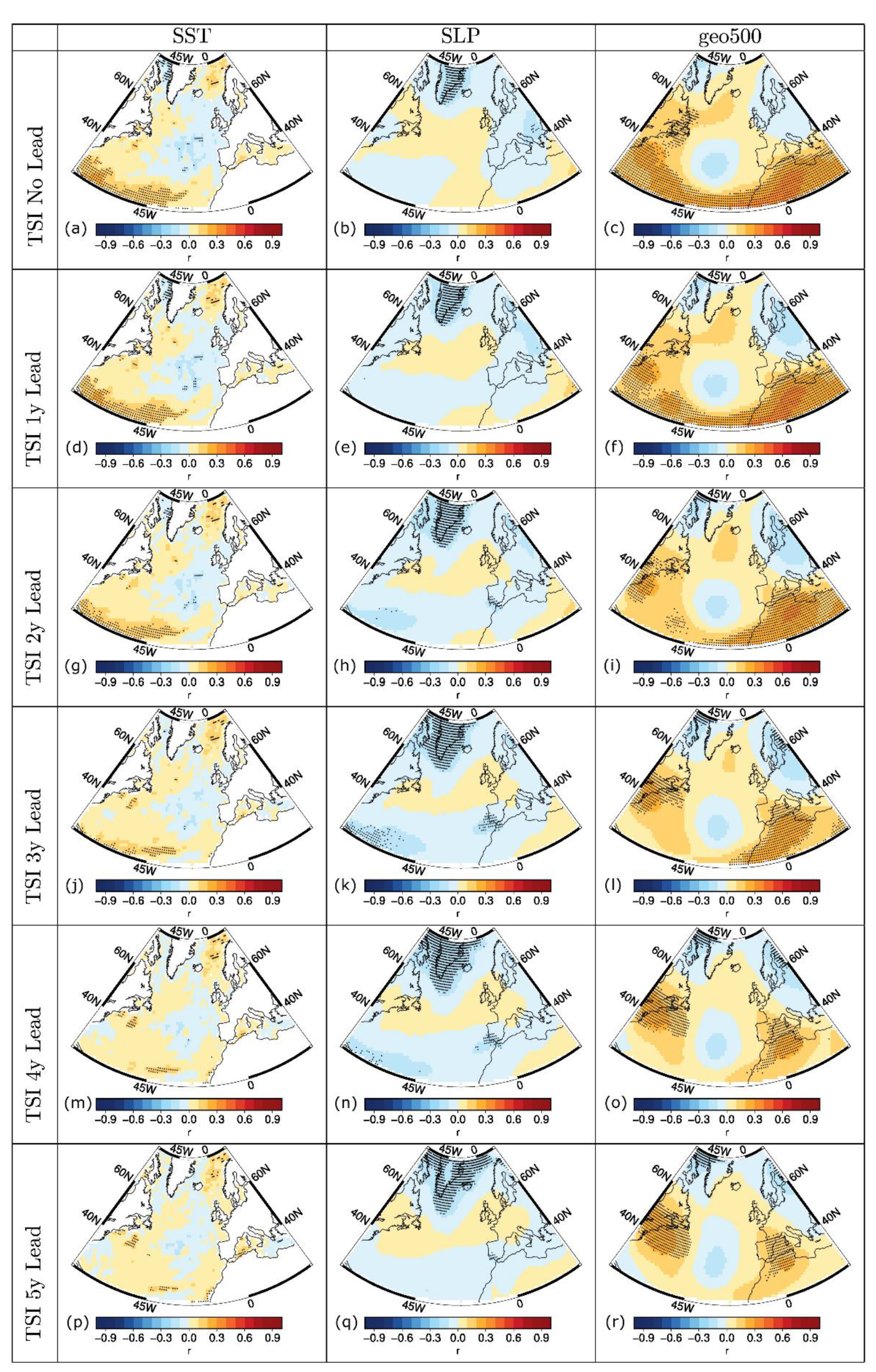
  • The statistical methods used indicate similar results for the CESM tropospheric forced response, agreeing on a weak response with decreased SLP over Greenland (−0.1 hPa per TSI SD) and increased geo500 over the subtropics (+0.8 gpm per TSI SD). This response is weak at all lags studied, with the values of the correlation coefficient being r = 0.1 for SLP and r = 0.3 for geo500.
  • The solar signal was not robustly identified during the preindustrial period in the summer SSTs of the CESM ensemble mean over the NA basin. This result was indicated by linear methods and composite analysis, and further justified from the analysis of the PiControl simulations.
  • The investigation of the CESM individual ensemble members signified that, for the low TSI scaling, model internal variability is larger than the changes induced by TSI forcing in single model simulations regarding surface and tropospheric variables. This result is further supported by the SNR values being lower than 0.4 for the climatic variables studied.
  • The control simulations of the two ESMs used in our study indicate that spurious correlation patterns between climatic variables and TSI may arise with linear regression, Pearson correlation, and composite analysis when using single model simulations.

Supplementary Materials

The following are available online at https://www.mdpi.com/article/10.3390/atmos12050568/s1, Figure S1: Signal-to-noise ratio (SNR), calculated for the CESM forced simulations as the ratio of the ensemble spread to the ensemble mean standard deviation. The calculation follows the method described in Jerez et al. [95]. The SNR is shown for (a) SST, (b) SLP, and (c) geo500., Figure S2: Correlation patterns between TSI and the SST (column 1), the SLP (column 2) and the geo500 (column 3). The results are given in the first, second, third and fourth row for the realizations E1, E2, E3 and E4 of the CESM forced simulations. The hatched areas indicate statistical significance at the 5% level. Figure S3: Correlation patterns between TSI and the SST (column 1), the SLP (column 2) and the geo500 (column 3) for the MPI-ESM-P (row 1) and CESM (row 2) control simulations. The hatched areas indicate statistical significance at the 5% level. Figure S4: Correlation patterns between TSI and U200 for the MPI-ESM-P (column 1) and CESM (column 2) forced simulations. The hatched areas indicate statistical significance at the 5% level. The correlation is given in the first row for no lead-time. As the row number increases, the TSI lead time increases by one year., Figure S5: Correlation patterns between TSI and U200 for the MPI-ESM-P (row 1) and CESM (row 2) control simulations., Figure S6: Composite patterns for high TSI minus low TSI periods for the SST (column 1), the SLP (column 2) and the geo500 (column 3) for the MPI-ESM-P (row 1) and CESM (row2) control simulations. The hatched areas indicate statistical significance at the 5% level. Figure S7: Correlation patterns between the SST (column 1), the SLP (column 2) and geo500 (column 3) of the individual CESM ensemble members pairs, for the period 850–1849 AD. The parameters are 11-year low-pass filtered and the hatched areas indicate statistical significance at the 5% level. Figure S8: Composite patterns for high TSI minus low TSI periods for the SST (column 1), the SLP (column 2) and the geo500 (column 3). The results are given in the first, second, third and fourth row for the realizations E1, E2, E3 and E4 of the CESM forced simulations. The hatched areas indicate statistical significance at the 5% level.

Author Contributions

The analysis was performed by M.P. with the consultation of S.W. and E.Z., while E.M.-C. conducted the MPI-ESM solar-only forced simulation. M.P. prepared the paper with contributions from all coauthors. All authors have read and agreed to the published version of the manuscript.

Funding

This research partly received external funding from the framework of the European Initial Marie Curie Training network ARAMACC (Annually resolved Archives of Marine Climate Change). This project has received funding from the European Union’s Seventh Framework Programme for research, technological development and demonstration under grant agreement no 604802.

Data Availability Statement

The CESM-LME output can be downloaded by the Earth System Grid at NCAR: https://www.earthsystemgrid.org/dataset/ucar.cgd.ccsm4.CESM_CAM5_LME.html (accessed on 20 January 2019).

Acknowledgments

The authors thank the CESM modelling group for providing their data.

Conflicts of Interest

The authors declare no competing interests.

References

  1. Mitchell, J.F.B.K.D.; Hegrel, G.C.; Zwiers, F.W.; Allen, M.R.; Marengo, J. Chapter 3 Detection of climate change and attribution of causes. In Climate Change 2001: The Scientific Basis; Houghton, J.T., Ding, Y., Griggs, D.J., Noguer, M., van der Linden, P.J., Dai, X., Maskell, K., Johnson, C.A., Eds.; Cambridge University Press: Cambridge, UK, 2001; pp. 696–738. [Google Scholar]
  2. Crowley, T.J. Causes of climate change over the past 1000 years. Science 2000, 289, 270–277. [Google Scholar] [CrossRef] [Green Version]
  3. Free, M.; Robock, A. Global warming in the context of the Little Ice Age. J. Geophys. Res. Atmos. 1999, 104, 19057–19070. [Google Scholar] [CrossRef]
  4. Hegerl, G.C.; Crowley, T.J.; Hyde, W.T.; Frame, D.J. Climate sensitivity constrained by temperature reconstructions over the past seven centuries. Nature 2006, 440, 1029–1032. [Google Scholar] [CrossRef] [PubMed]
  5. Shindell, D.T.; Schmidt, G.A.; Miller, R.L.; Mann, M.E. Volcanic and solar forcing of climate change during the preindustrial era. J. Clim. 2003, 16, 4094–4107. [Google Scholar] [CrossRef]
  6. Haigh, J.D. The role of stratospheric ozone in modulating the solar radiative forcing of climate. Nature 1994, 370, 544. [Google Scholar] [CrossRef]
  7. Lean, J. The Sun’s variable radiation and its relevance for Earth. Annu. Rev. Astron. Astrophys. 1997, 35, 33–67. [Google Scholar] [CrossRef]
  8. Lilensten, J.; De Wit, T.D.; Matthes, K. Earth’s Climate Response to a Changing Sun: A Review of the Current Understanding by the European Research Group TOSCA; EDP Sciences: Paris, France, 2016. [Google Scholar]
  9. Seppälä, A.; Clilverd, M.A. Energetic particle forcing of the Northern Hemisphere winter stratosphere: Comparison to solar irradiance forcing. Front. Phys. 2014, 2, 25. [Google Scholar] [CrossRef] [Green Version]
  10. Shindell, D.; Rind, D.; Balachandran, N.; Lean, J.; Lonergan, P. Solar cycle variability, ozone, and climate. Science 1999, 284, 305–308. [Google Scholar] [CrossRef] [Green Version]
  11. Matthes, K.; Funke, B.; Andersson, M.E.; Barnard, L.; Beer, J.; Charbonneau, P.; Clilverd, M.A.; de Wit, T.D.; Haberreiter, M.; Hendry, A.; et al. Solar forcing for CMIP6 (v3. 2). Geosci. Model Dev. 2017, 10, 2247–2302. [Google Scholar] [CrossRef] [Green Version]
  12. Eddy, J.A. The maunder minimum. Science 1976, 192, 1189–1202. [Google Scholar] [CrossRef] [Green Version]
  13. Chiodo, G.; García-Herrera, R.; Calvo, N.; Vaquero, J.M.; Añel, J.A.; Barriopedro, D.; Matthes, K. The impact of a future solar minimum on climate change projections in the Northern Hemisphere. Environ. Res. Lett. 2016, 11, 034015. [Google Scholar] [CrossRef]
  14. Ermolli, I.; Matthes, K.; de Wit, T.D.; Krivova, N.A.; Tourpali, K.; Weber, M.; Unruh7, Y.C.; Gray, L.; Langematz, U.; Pilewskie, P.; et al. Recent variability of the solar spectral irradiance and its impact on climate modelling. Atmos. Chem. Phys. 2013, 13, 3945–3977. [Google Scholar] [CrossRef] [Green Version]
  15. Haigh, J.D. The Sun and the Earth’s climate. Living Rev. Sol. Phys. 2007, 4, 1–64. [Google Scholar] [CrossRef] [Green Version]
  16. Ineson, S.; Maycock, A.C.; Gray, L.J.; Scaife, A.A.; Dunstone, N.J.; Harder, J.W.; Knight, J.R.; Lockwood, M.; Manners, J.C.; Wood, R.A. Regional climate impacts of a possible future grand solar minimum. Nat. Commun. 2015, 6, 7535. [Google Scholar] [CrossRef] [PubMed]
  17. Fligge, M.; Solanki, S. The solar spectral irradiance since 1700. Geophys. Res. Lett. 2000, 27, 2157–2160. [Google Scholar] [CrossRef] [Green Version]
  18. Vieira, L.E.A.; Solanki, S.K.; Krivova, N.A.; Usoskin, I. Evolution of the solar irradiance during the Holocene. Astron. Astrophys. 2011, 531, A6. [Google Scholar] [CrossRef] [Green Version]
  19. Wang, Y.-M.; Lean, J.; Sheeley Jr, N. Modeling the Sun’s magnetic field and irradiance since 1713. Astrophys. J. 2005, 625, 522. [Google Scholar] [CrossRef]
  20. Kopp, G.; Lean, J.L. A new, lower value of total solar irradiance: Evidence and climate significance. Geophys. Res. Lett. 2011, 38. [Google Scholar] [CrossRef] [Green Version]
  21. Prša, A.; Harmanec, P.; Torres, G.; Mamajek, E.; Asplund, M.; Capitaine, N.; Christensen-Dalsgaard, J.; Depagne, É.; Haberreiter, M.; Hekker, S.; et al. Nominal values for selected solar and planetary quantities: IAU 2015 Resolution B3. Astron. J. 2016, 152, 41. [Google Scholar] [CrossRef]
  22. Enfield, D.B.; Mestas-Nuñez, A.M.; Trimble, P.J. The Atlantic multidecadal oscillation and its relation to rainfall and river flows in the continental US. Geophys. Res. Lett. 2001, 28, 2077–2080. [Google Scholar] [CrossRef] [Green Version]
  23. Hurrell, J.W.; Folland, C.K. A change in the summer atmospheric circulation over the North Atlantic. Clivar Exch. 2002, 25, 52–54. [Google Scholar]
  24. Sutton, R.T.; Dong, B. Atlantic Ocean influence on a shift in European climate in the 1990s. Nat. Geosci. 2012, 5, 788. [Google Scholar] [CrossRef]
  25. Fritts, H. Tree Rings and Climate; Elsevier: Amsterdam, The Netherlands, 2012. [Google Scholar]
  26. Schöne, B.R.; Houk, S.D.; Freyre Castro, A.D.; Fiebig, J.; Oschmann, W.; Kröncke, I.; Dreyer, W.; Gosselck, F. Daily growth rates in shells of Arctica islandica: Assessing sub-seasonal environmental controls on a long-lived bivalve mollusk. Palaios 2005, 20, 78–92. [Google Scholar] [CrossRef]
  27. Pyrina, M. North Atlantic Ocean Decadal Variability Over the Past Millennium from Climate Model Simulations and Proxy Based Reconstructions. Ph.D. Thesis, University of Hamburg, Hamburg, Germany, 2017. [Google Scholar]
  28. Hegerl, G.C.; Crowley, T.J.; Baum, S.K.; Kim, K.Y.; Hyde, W.T. Detection of volcanic, solar and greenhouse gas signals in paleo-reconstructions of Northern Hemispheric temperature. Geophys. Res. Lett. 2003, 30. [Google Scholar] [CrossRef] [Green Version]
  29. Swingedouw, D.; Terray, L.; Cassou, C.; Voldoire, A.; Salas-Mélia, D.; Servonnat, J. Natural forcing of climate during the last millennium: Fingerprint of solar variability. Clim. Dyn. 2011, 36, 1349–1364. [Google Scholar] [CrossRef]
  30. Wang, Z.; Wang, J.; Zhang, S. Variations of the global annual mean surface temperature during the past 2000 years: Results from the CESM1. Theor. Appl. Climatol. 2019, 137, 2877–2887. [Google Scholar] [CrossRef]
  31. Lean, J.L.; Rind, D.H. How natural and anthropogenic influences alter global and regional surface temperatures: 1889 to 2006. Geophys. Res. Lett. 2008, 35. [Google Scholar] [CrossRef] [Green Version]
  32. Reynolds, D.J.; Scourse, J.D.; Halloran, P.R.; Nederbragt, A.J.; Wanamaker, A.D.; Butler, P.G.; Richardson, C.A.; Heinemeier, J.; Eiriksson, J.; Knudsen, K.L.; et al. Annually resolved North Atlantic marine climate over the last millennium. Nat. Commun. 2016, 7, 13502. [Google Scholar] [CrossRef] [Green Version]
  33. Sejrup, H.; Lehman, S.J.; Haflidason, H.; Noone, D.; Muscheler, R.; Berstad, I.M.; Andrews, J.T. Response of Norwegian Sea temperature to solar forcing since 1000 AD. J. Geophys. Res. Ocean. 2010, 115. [Google Scholar] [CrossRef] [Green Version]
  34. Chen, H.; Ma, H.; Li, X.; Sun, S. Solar influences on spatial patterns of Eurasian winter temperature and atmospheric general circulation anomalies. J. Geophys. Res. Atmos. 2015, 120, 8642–8657. [Google Scholar] [CrossRef] [Green Version]
  35. Salby, M.L.; Callaghan, P.F. Evidence of the solar cycle in the tropical troposphere. J. Geophys. Res. Atmos. 2006, 111. [Google Scholar] [CrossRef] [Green Version]
  36. Sfîcă, L.; Iordache, I.; Voiculescu, M. Solar signal on regional scale: A study of possible solar impact upon Romania’s climate. J. Atmos. Sol. Terr. Phys. 2018, 177, 257–265. [Google Scholar] [CrossRef]
  37. van Loon, H.; Meehl, G.A.; Arblaster, J.M. A decadal solar effect in the tropics in July–August. J. Atmos. Sol. Terr. Phys. 2004, 66, 1767–1778. [Google Scholar] [CrossRef]
  38. Jiang, H.; Eiríksson, J.; Schulz, M.; Knudsen, K.-L.; Seidenkrantz, M.-S. Evidence for solar forcing of sea-surface temperature on the North Icelandic Shelf during the late Holocene. Geology 2005, 33, 73–76. [Google Scholar] [CrossRef]
  39. Moffa-Sánchez, P.; Born, A.; Hall, I.R.; Thornalley, D.J.; Barker, S. Solar forcing of North Atlantic surface temperature and salinity over the past millennium. Nat. Geosci. 2014, 7, 275. [Google Scholar] [CrossRef]
  40. Lockwood, M. Solar influence on global and regional climates. Surv. Geophys. 2012, 33, 503–534. [Google Scholar] [CrossRef] [Green Version]
  41. Le, T.; Sjolte, J.; Muscheler, R. The influence of external forcing on subdecadal variability of regional surface temperature in CMIP5 simulations of the last millennium. J. Geophys. Res. Atmos. 2016, 121, 1671–1682. [Google Scholar] [CrossRef] [Green Version]
  42. Misios, S.; Mitchell, D.M.; Gray, L.J.; Tourpali, K.; Matthes, K.; Hood, L.; Schmidt, H.; Chiodo, G.; Thiéblemont, R.; Rozanov, E.; et al. Solar signals in CMIP-5 simulations: Effects of atmosphere–ocean coupling. Q. J. R. Meteorol. Soc. 2016, 142, 928–941. [Google Scholar] [CrossRef]
  43. Mitchell, D.; Misios, S.; Gray, L.J.; Tourpali, K.; Matthes, K.; Hood, L.; Schmidt, H.; Chiodo, G.; Thieblemont, R.; Rozanov, E.; et al. Solar signals in CMIP-5 simulations: The stratospheric pathway. Q. J. R. Meteorol. Soc. 2015, 141, 2390–2403. [Google Scholar] [CrossRef] [Green Version]
  44. Thiéblemont, R.; Matthes, K.; Omrani, N.-E.; Kodera, K.; Hansen, F. Solar forcing synchronizes decadal North Atlantic climate variability. Nat. Commun. 2015, 6, 8268. [Google Scholar] [CrossRef] [Green Version]
  45. Jungclaus, J.H.; Lohmann, K.; Zanchettin, D. Enhanced 20th century heat transfer to the Arctic simulated in context of climate variations over last millennium. Clim. Past 2014, 10, 2201–2213. [Google Scholar] [CrossRef] [Green Version]
  46. Schmidt, G.A.; Jungclaus, J.H.; Ammann, C.M.; Bard, E.; Braconnot, P.C.; Crowley, T.J.; Delaygue, G.; Joos, F.; Krivova, N.A.; Muscheler, R.; et al. Climate forcing reconstructions for use in PMIP simulations of the last millennium (v1. 0). Geosci. Model Dev. 2011. [Google Scholar] [CrossRef] [Green Version]
  47. Stevens, B.; Giorgetta, M.; Esch, M.; Mauritsen, T.; Crueger, T.; Rast, S.; Salzmann, M.; Schmidt, H.; Bader, J.; Block, K. Atmospheric component of the MPI-M Earth System Model: ECHAM6. J. Adv. Model. Earth Syst. 2013, 5, 146–172. [Google Scholar] [CrossRef]
  48. Jungclaus, J.; Fischer, N.; Haak, H.; Lohmann, K.; Marotzke, J.; Matei, D.; Mikolajewicz, U.; Notz, D.; Storch, J. Characteristics of the ocean simulations in the Max Planck Institute Ocean Model (MPIOM) the ocean component of the MPI-Earth system model. J. Adv. Model. Earth Syst. 2013, 5, 422–446. [Google Scholar] [CrossRef]
  49. Giorgetta, M.A.; Jungclaus, J.; Reick, C.H.; Legutke, S.; Bader, J.; Böttinger, M.; Brovkin, V.; Crueger, T.; Esch, M.; Fieg, K. Climate and carbon cycle changes from 1850 to 2100 in MPI-ESM simulations for the Coupled Model Intercomparison Project phase 5. J. Adv. Model. Earth Syst. 2013, 5, 572–597. [Google Scholar] [CrossRef]
  50. Kinne, S.; O’Donnel, D.; Stier, P.; Kloster, S.; Zhang, K.; Schmidt, H.; Rast, S.; Giorgetta, M.; Eck, T.F.; Stevens, B. MAC-v1: A new global aerosol climatology for climate studies. J. Adv. Model. Earth Syst. 2013, 5, 704–740. [Google Scholar] [CrossRef]
  51. Lohmann, K.; Mignot, J.; Langehaug, H.R.; Jungclaus, J.H.; Matei, D.; Otterå, O.H.; Gao, Y.; Mjell, T.L.; Ninnemann, U.S.; Kleiven, H.F. Using simulations of the last millennium to understand climate variability seen in palaeo-observations: Similar variation of Iceland–Scotland overflow strength and Atlantic Multidecadal Oscillation. Clim. Past Discuss. 2015, 11, 203–216. [Google Scholar] [CrossRef] [Green Version]
  52. Otto-Bliesner, B.L.; Brady, E.C.; Fasullo, J.; Jahn, A.; Landrum, L.; Stevenson, S.; Rosenbloom, N.; Mai, A.; Strand, G. Climate variability and change since 850 CE: An ensemble approach with the community earth system model. Bull. Am. Meteorol. Soc. 2016, 97, 735–754. [Google Scholar] [CrossRef]
  53. Hurrell, J.W.; Holland, M.M.; Gent, P.R.; Ghan, S.; Kay, J.E.; Kushner, P.J.; Lamarque, J.-F.; Large, W.G.; Lawrence, D.; Lindsay, K. The community earth system model: A framework for collaborative research. Bull. Am. Meteorol. Soc. 2013, 94, 1339–1360. [Google Scholar] [CrossRef]
  54. Mills, M.J.; Schmidt, A.; Easter, R.; Solomon, S.; Kinnison, D.E.; Ghan, S.J.; Neely III, R.R.; Marsh, D.R.; Conley, A.; Bardeen, C.G. Global volcanic aerosol properties derived from emissions, 1990–2016, 2014, using CESM1 (WACCM). J. Geophys. Res. Atmos. 2016, 121, 2332–2348. [Google Scholar] [CrossRef] [Green Version]
  55. Iacono, M.J.; Delamere, J.S.; Mlawer, E.J.; Shephard, M.W.; Clough, S.A.; Collins, W.D. Radiative forcing by long-lived greenhouse gases: Calculations with the AER radiative transfer models. J. Geophys. Res. Atmos. 2008, 113. [Google Scholar] [CrossRef]
  56. Neale, R.B.; Chen, C.-C.; Gettelman, A.; Lauritzen, P.H.; Park, S.; Williamson, D.L.; Conley, A.J.; Garcia, R.; Kinnison, D.; Lamarque, J.-F. Description of the NCAR Community Atmosphere Model (CAM 5.0); NCAR Technical Note NCAR/TN-486+ STR; NCAR: Boulder, CO, USA, 2010; pp. 1–12. [Google Scholar]
  57. Chervin, R.M. Interannual variability and seasonal climate predictability. J. Atmos. Sci. 1986, 43, 233–251. [Google Scholar] [CrossRef] [Green Version]
  58. Dütsch, H. Vertical ozone distribution on a global scale. Pure Appl. Geophys. 1978, 116, 511–529. [Google Scholar] [CrossRef]
  59. Schulzweida, U.; Müller, R.; Kornblüh, L.; Ansorge, C.; Quast, R. CDO–Climate Data Operators–v1. 5.9; Center for Marine and Atmos. Sciences (ZMAW), Max-Planck Institute for Meteorology, University of Hamburg: Hamburg, Germany, 2012; Available online: https://code.zmaw.de/projects/cdo (accessed on 20 January 2019).
  60. Gray, L.J.; Scaife, A.A.; Mitchell, D.M.; Osprey, S.; Ineson, S.; Hardiman, S.; Butchart, N.; Knight, J.; Sutton, R.; Kodera, K. A lagged response to the 11 year solar cycle in observed winter Atlantic/European weather patterns. J. Geophys. Res. Atmos. 2013, 118, 13405–413420. [Google Scholar] [CrossRef] [Green Version]
  61. Ebisuzaki, W. A method to estimate the statistical significance of a correlation when the data are serially correlated. J. Clim. 1997, 10, 2147–2153. [Google Scholar] [CrossRef]
  62. Schreiber, T.; Schmitz, A. Improved surrogate data for nonlinearity tests. Phys. Rev. Lett. 1996, 77, 635. [Google Scholar] [CrossRef] [PubMed] [Green Version]
  63. Maher, N.; Matei, D.; Milinski, S.; Marotzke, J. ENSO change in climate projections: Forced response or internal variability? Geophys. Res. Lett. 2018, 45, 11,390–11,398. [Google Scholar] [CrossRef]
  64. Meehl, G.A.; Arblaster, J.M.; Matthes, K.; Sassi, F.; van Loon, H. Amplifying the Pacific climate system response to a small 11-year solar cycle forcing. Science 2009, 325, 1114–1118. [Google Scholar] [CrossRef] [Green Version]
  65. Gray, L.J.; Beer, J.; Geller, M.; Haigh, J.D.; Lockwood, M.; Matthes, K.; Cubasch, U.; Fleitmann, D.; Harrison, G.; Hood, L. Solar influences on climate. Rev. Geophys. 2010, 48. [Google Scholar] [CrossRef]
  66. Kodera, K.; Kuroda, Y. Dynamical response to the solar cycle. J. Geophys. Res. Atmos. 2002, 107. [Google Scholar] [CrossRef] [Green Version]
  67. Dima, M.; Voiculescu, M. Global patterns of solar influence on high cloud cover. Clim. Dyn. 2016, 47, 667–678. [Google Scholar] [CrossRef]
  68. Meehl, G.A.; Arblaster, J.M.; Branstator, G.; Van Loon, H. A coupled air–sea response mechanism to solar forcing in the Pacific region. J. Clim. 2008, 21, 2883–2897. [Google Scholar] [CrossRef] [Green Version]
  69. White, W.B.; Lean, J.; Cayan, D.R.; Dettinger, M.D. Response of global upper ocean temperature to changing solar irradiance. J. Geophys. Res. Oceans 1997, 102, 3255–3266. [Google Scholar] [CrossRef]
  70. Jin, C.; Wang, B.; Liu, J.; Ning, L.; Yan, M. Decadal variability of northern Asian winter monsoon shaped by the 11-year solar cycle. Clim. Dyn. 2019, 53, 6559–6568. [Google Scholar] [CrossRef] [Green Version]
  71. Ammann, C.M.; Joos, F.; Schimel, D.S.; Otto-Bliesner, B.L.; Tomas, R.A. Solar influence on climate during the past millennium: Results from transient simulations with the NCAR Climate System Model. Proc. Natl. Acad. Sci. USA 2007, 104, 3713–3718. [Google Scholar] [CrossRef] [Green Version]
  72. Gray, L.; Woollings, T.; Andrews, M.; Knight, J. Eleven-year solar cycle signal in the NAO and Atlantic/European blocking. Q. J. R. Meteorol. Soc. 2016, 142, 1890–1903. [Google Scholar] [CrossRef] [Green Version]
  73. Scaife, A.A.; Ineson, S.; Knight, J.R.; Gray, L.; Kodera, K.; Smith, D.M. A mechanism for lagged North Atlantic climate response to solar variability. Geophys. Res. Lett. 2013, 40, 434–439. [Google Scholar] [CrossRef]
  74. Yukimoto, S.; Kodera, K.; Thiéblemont, R. Delayed North Atlantic Response to Solar Forcing of the Stratospheric Polar Vortex. SOLA 2017, 13, 53–58. [Google Scholar] [CrossRef] [Green Version]
  75. Turner, T.E.; Swindles, G.T.; Charman, D.J.; Langdon, P.G.; Morris, P.J.; Booth, R.K.; Parry, L.E.; Nichols, J.E. Solar cycles or random processes? Evaluating solar variability in Holocene climate records. Sci. Rep. 2016, 6, 23961. [Google Scholar] [CrossRef] [PubMed] [Green Version]
  76. Blaauw, M.; Van Geel, B.; Van Der Plicht, J. Solar forcing of climatic change during the mid-Holocene: Indications from raised bogs in The Netherlands. Holocene 2004, 14, 35–44. [Google Scholar] [CrossRef] [Green Version]
  77. Nichols, J.E.; Huang, Y. Hydroclimate of the northeastern United States is highly sensitive to solar forcing. Geophys. Res. Lett. 2012, 39. [Google Scholar] [CrossRef] [Green Version]
  78. Swindles, G.T.; Patterson, R.T.; Roe, H.M.; Galloway, J.M. Evaluating periodicities in peat-based climate proxy records. Quat. Sci. Rev. 2012, 41, 94–103. [Google Scholar] [CrossRef]
  79. Harrison, S.P.; Bartlein, P.J.; Prentice, I.C. What have we learnt from palaeoclimate simulations? J. Quat. Sci. 2016, 31, 363–385. [Google Scholar] [CrossRef] [Green Version]
  80. Harrison, S.P.; Bartlein, P.; Izumi, K.; Li, G.; Annan, J.; Hargreaves, J.; Braconnot, P.; Kageyama, M. Evaluation of CMIP5 palaeo-simulations to improve climate projections. Nat. Clim. Chang. 2015, 5, 735–743. [Google Scholar] [CrossRef]
  81. Ludwig, P.; Gómez-Navarro, J.J.; Pinto, J.G.; Raible, C.C.; Wagner, S.; Zorita, E. Perspectives of regional paleoclimate modeling. Ann. N. Y. Acad. Sci. 2019, 1436, 54. [Google Scholar] [CrossRef] [PubMed] [Green Version]
  82. Lovejoy, S.; Varotsos, C. Scaling regimes and linear/nonlinear responses of last millennium climate to volcanic and solar forcings. Earth Syst. Dyn. 2016, 7, 133–150. [Google Scholar] [CrossRef] [Green Version]
  83. Adolphi, F.; Muscheler, R.; Svensson, A.; Aldahan, A.; Possnert, G.; Beer, J.; Sjolte, J.; Björck, S.; Matthes, K.; Thiéblemont, R. Persistent link between solar activity and Greenland climate during the Last Glacial Maximum. Nat. Geosci. 2014, 7, 662–666. [Google Scholar] [CrossRef]
  84. Saarni, S.; Muschitiello, F.; Weege, S.; Brauer, A.; Saarinen, T. A late Holocene record of solar-forced atmospheric blocking variability over Northern Europe inferred from varved lake sediments of Lake Kuninkaisenlampi. Quat. Sci. Rev. 2016, 154, 100–110. [Google Scholar] [CrossRef]
  85. Davini, P.; Cagnazzo, C.; Neale, R.; Tribbia, J. Coupling between Greenland blocking and the North Atlantic Oscillation pattern. Geophys. Res. Lett. 2012, 39. [Google Scholar] [CrossRef] [Green Version]
  86. Woollings, T.; Lockwood, M.; Masato, G.; Bell, C.; Gray, L. Enhanced signature of solar variability in Eurasian winter climate. Geophys. Res. Lett. 2010, 37. [Google Scholar] [CrossRef]
  87. Barriopedro, D.; García-Herrera, R.; Huth, R. Solar modulation of Northern Hemisphere winter blocking. J. Geophys. Res. Atmos. 2008, 113. [Google Scholar] [CrossRef] [Green Version]
  88. Ineson, S.; Scaife, A.A.; Knight, J.R.; Manners, J.C.; Dunstone, N.J.; Gray, L.J.; Haigh, J.D. Solar forcing of winter climate variability in the Northern Hemisphere. Nat. Geosci. 2011, 4, 753–757. [Google Scholar] [CrossRef] [Green Version]
  89. Xoplaki, E.; Trigo, R.; García-Herrera, R.; Barriopedro, D.; D’Andrea, F.; Fischer, E.; Gimeno, L.; Gouveia, C.; Hernández, E.; Kuglitsch, F. The Climate of the Mediterranean Region; Elsevier: Amsterdam, The Netherlands, 2012; Chapter 6; pp. 347–417. [Google Scholar]
  90. Strestik, J. Solar Variability as an Input to the Earth’s Environment. In Proceedings of the International Solar Cycle Studies (ISCS) Symposium 2003, Tatranská Lomnica, Slovakia, 23–28 June 2003; pp. 393–396. [Google Scholar]
  91. Zambri, B.; Robock, A. Winter warming and summer monsoon reduction after volcanic eruptions in Coupled Model Intercomparison Project 5 (CMIP5) simulations. Geophys. Res. Lett. 2016, 43, 10920–10928. [Google Scholar] [CrossRef]
  92. Cai, M.; Tung, K.-K. Robustness of dynamical feedbacks from radiative forcing: 2% solar versus 2× CO2 experiments in an idealized GCM. J. Atmos. Sci. 2012, 69, 2256–2271. [Google Scholar] [CrossRef]
  93. Misios, S.; Schmidt, H. The role of the oceans in shaping the tropospheric response to the 11 year solar cycle. Geophys. Res. Lett. 2013, 40, 6373–6377. [Google Scholar] [CrossRef] [Green Version]
  94. Ortega, P.; Lehner, F.; Swingedouw, D.; Masson-Delmotte, V.; Raible, C.C.; Casado, M.; Yiou, P. A model-tested North Atlantic Oscillation reconstruction for the past millennium. Nature 2015, 523, 71–74. [Google Scholar] [CrossRef]
  95. Jerez, S.; Montavez, J.P.; Jimenez-Guerrero, P.; Gomez-Navarro, J.J.; Lorente-Plazas, R.; Zorita, E. A multi-physics ensemble of present-day climate regional simulations over the Iberian Peninsula. Clim. Dyn. 2013, 40, 3023–3046. [Google Scholar] [CrossRef]
Figure 1. (a) Standardized TSI anomalies for the period 850–1849 AD, and (b) TSI anomalies for the period 850–1849 AD as a function of frequency. The data regard the Vieira et al. [18] TSI reconstruction over the Holocene.
Atmosphere 12 00568 g001
Figure 2. Correlation patterns between TSI and the SST (a,d), the SLP (b,e) and the geo500 (c,f) for the MPI-ESM-P (ac) and CESM ensemble mean (df). The hatched areas indicate statistical significance at the 5% level. The range of r-values for SST, SLP and geo500 is approximately ±0.3, ±0.2, and ±0.4, respectively.
Atmosphere 12 00568 g002
Figure 3. Regression patterns between TSI and the SST (a,d), the SLP (b,e) and the geo500 (c,f) for the MPI-ESM-P (ac) and CESM ensemble mean (df). The hatched areas indicate statistical significance at the 5% level.
Atmosphere 12 00568 g003
Figure 4. Correlation patterns between TSI and the SST (a,d,g,j,m,p), the SLP (b,e,h,k,n,q) and the geo500 (c,f,i,l,o,r) for the MPI-ESM-P. The correlation is given in the first row for no lead-time. As the row number increases, the TSI lead time increases by one year. The hatched areas indicate statistical significance at the 5% level. The range of r-values for SSTs, SLP and geo500 is approximately ±0.3, ±0.2, and ±0.4, respectively.
Atmosphere 12 00568 g004
Figure 5. Correlation patterns between TSI and the SST (a,d,g,j,m,p), the SLP (b,e,h,k,n,q) and the geo500 (c,f,i,l,o,r) for the CESM ensemble mean. The correlation is given in the first row for no lead-time. As the row number increases, the TSI lead time increases by one year. The hatched areas indicate statistical significance at the 5% level. The range of r-values for SSTs, SLP and geo500 is approximately ±0.3, ±0.2, and ±0.4, respectively.
Atmosphere 12 00568 g005
Figure 6. Composite patterns for high TSI minus low TSI periods for the SST (a,d), the SLP (b,e) and the geo500 (c,f) for the MPI-ESM-P (ac) and CESM ensemble mean (df). The hatched areas indicate statistical significance at the 5% level.
Atmosphere 12 00568 g006
Table 1. Details on the models and experiments used in this study.
ModelMPI-ESM-PCESM1-CAM5
Institute (country)MPI-M (Germany)NSF-DOE-NCAR (USA)
High Top (H)—Low Top (L) classificationHL
Ozone ImplementationPrescribed (but scales with the strength of the TSI variation)Semi-Offline
Number of simulations/
simulation name, and forcings used for the solar-only forcing experiments
1/MPI-R1
Solar forcing [18], Orbital forcing parameters and well mixed-greenhouse gases [46]
4/E1, E2, E3, E4
Solar forcing [18], Orbital forcing parameters and well mixed-greenhouse gases [46]
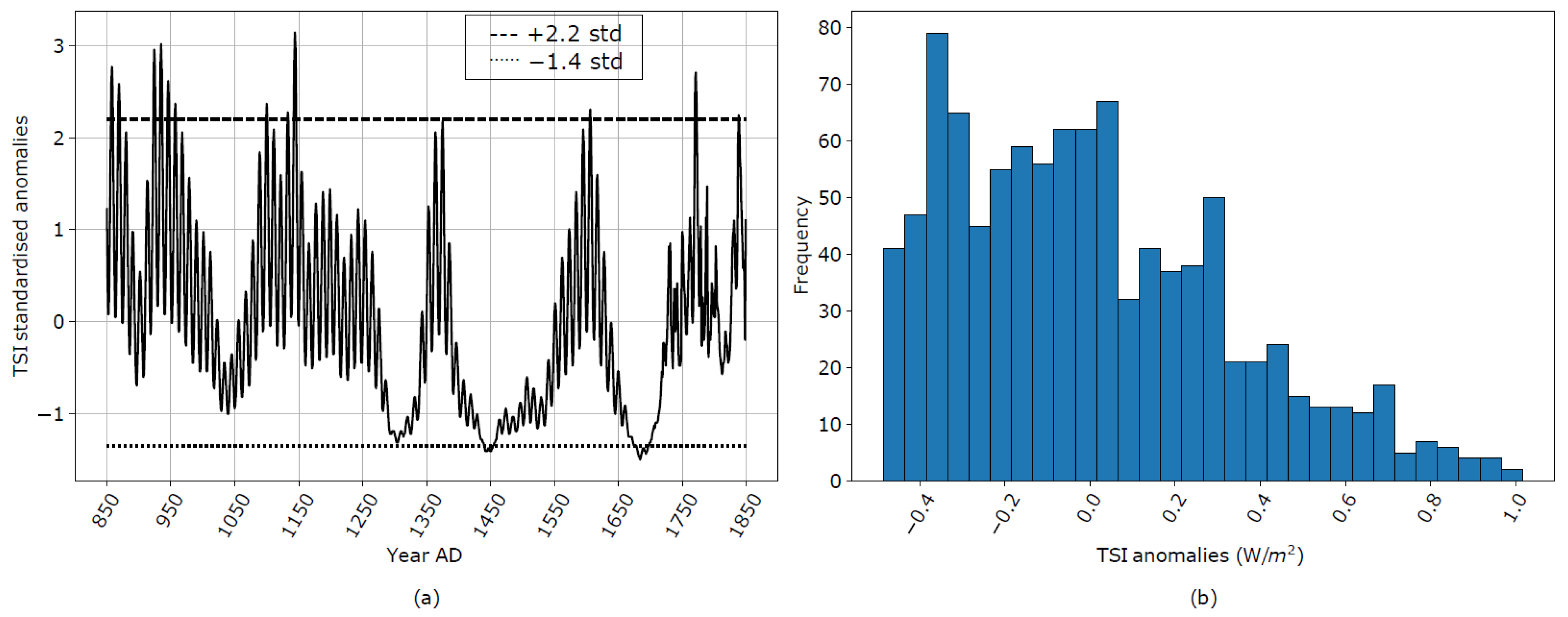
Table 2. Details on the years with TSI anomalies exceeding, by 2.2, the standard deviation value (column 1) and with negative TSI anomalies exceeding 1.4 times the standard deviation value (column 2).
Years with TSI > 2.2 SDYears with TSI < –1.4 SD
857, 858, 859, 868, 869, 870, 923, 924, 925, 934, 935, 936, 945, 946, 947, 957, 1100, 1133, 1143, 1144, 1145, 1606, 1770, 1771, 17721442, 1443, 1444, 1445, 1449, 1450, 1451, 1680, 1681, 1682, 1683, 1684, 1685, 1686, 1687, 1691, 1692, 1693, 1694, 1695
Publisher’s Note: MDPI stays neutral with regard to jurisdictional claims in published maps and institutional affiliations.

