Ambient Levels, Emission Sources and Health Effect of PM_2.5-Bound Carbonaceous Particles and Polycyclic Aromatic Hydrocarbons in the City of Kuala Lumpur, Malaysia

Abstract

With increasing interest in understanding the contribution of secondary organic aerosol (SOA) to particulate air pollution in urban areas, an exploratory study was carried out to determine levels of carbonaceous aerosols and polycyclic aromatic hydrocarbons (PAHs) in the city of Kuala Lumpur, Malaysia. PM_2.5 samples were collected using a high-volume sampler for 24 h in several areas in Kuala Lumpur during the north-easterly monsoon from January to March 2019. Samples were analyzed for water-soluble organic carbon (WSOC), organic carbon (OC), and elemental carbon (EC). Secondary organic carbon (SOC) in PM_2.5 was estimated. Particle-bound PAHs were analyzed using gas chromatography-flame ionization detector (GC-FID). Average concentrations of WSOC, OC, and EC were 2.73 ± 2.17 (range of 0.63–9.12) µg/m³, 6.88 ± 4.94 (3.12–24.1) µg/m³, and 3.68 ± 1.58 (1.33–6.82) µg/m³, respectively, with estimated average SOC of 2.33 µg/m³, contributing 34% to total OC. The dominance of char-EC over soot-EC suggests that PM_2.5 is influenced by biomass and coal combustion sources. The average of total PAHs was 1.74 ± 2.68 ng/m³. Source identification methods revealed natural gas and biomass burning, and urban traffic combustion as dominant sources of PAHs in Kuala Lumpur. A deterministic health risk assessment of PAHs was conducted for several age groups, including infant, toddler, children, adolescent, and adult. Carcinogenic and non-carcinogenic risk of PAH species were well below the acceptable levels recommended by the USEPA. Backward trajectory analysis revealed north-east air mass brought pollutants to the studied areas, suggesting the north-easterly monsoon as a major contributor to increased air pollution in Kuala Lumpur. Further work is needed using long-term monitoring data to understand the origin of PAHs contributing to SOA formation and to apply source-risk apportionment to better elucidate the potential risk factors posed by the various sources in urban areas in Kuala Lumpur.

1. Introduction

Urban air pollution is a potential cause for deleterious impact on public health and the environment. Several studies reported that there are excess deaths or global premature deaths in the urban and industrial areas due to air pollution [1,2,3]. The major causes of ambient air pollution are related to the rise in population, industrial activities and number of vehicles in cities [4,5,6,7].

Being a tiny air particle, PM_2.5 with an aerodynamic diameter equal to or less than 2.5 µm can easily penetrate deep into the human respiratory system [8] and have an influence on the increase of daily mortality and morbidity of adults caused by having breathing difficulties and the development of lung cancer [9]. While originating from primary and secondary sources [10], meteorological factors significantly influence PM_2.5 concentration at local and regional scales due to its smaller size and ability to be transported over long distances [11]. Studies by Dominick et al. [12], Rahim et al. [13], Mohyeddin et al. [14], and Farren et al. [15] found that north-easterly monsoons bring pollutants to East Coast Malaysia from South China Sea, particularly the East Asian region that has winter monsoon seasons and typically larger pollutants are emitted during that time as more fuel is used for heating in winter. Khan et al. [16] found a direction of north-easterly air mass bringing biomass burning pollutants to the sampling area located in Bangi, Selangor, Malaysia.

The major chemical compositions in PM_2.5 were elemental carbon (EC) and organic carbon (OC), ammonium sulfate and ammonium nitrate, and inorganic mineral components [10,17]. EC originates from the primary sources via the incomplete combustion processes whereas OC can come from both primary and secondary pathways [17]. Increasing the secondary organic aerosol (SOA) contribution to urban particulate air pollution is well-reported in literature [18,19,20]. The volatile PAHs are also a significant source of SOA [19,20]. Secondary organic carbon (SOC) is produced in the atmosphere via atmospheric processes, and can be estimated using the minimum ratio of OC/EC. Water-soluble organic carbon (WSOC), which is a part of SOC, is formed via the photochemical reaction of volatile organic carbon, and this WSOC can influence cloud formation [18]. The carbonaceous compounds consist of carcinogenic pollutants such as polycyclic aromatic hydrocarbons (PAHs) [21,22,23].

PAHs are environmentally persistent organic pollutants (POPs) that consist of two or more fused benzene rings [4,5,10]. According to Liu et al. [9], the PAHs concentration is higher in the respirable fraction of air particles than the larger fractions. PAHs are ubiquitous and semi-volatile, and are released into ambient air through the incomplete combustion of organic materials. Several studies reported that the predominant emission sources of PAHs are automobiles, industrial processes, domestic heating systems, waste incineration facilities, tobacco smoking, and several natural sources, including forest fires and volcanic eruptions [4,6,24,25,26,27,28]. Previous literature reported that vehicle emission, coal burning and biomass combustion were the principal sources of PAHs in PM_2.5 [29,30,31]. PAHs sources can be classified into two main groups, pyrogenic and petrogenic. Pyrogenic PAHs are formed from incomplete combustion of organic matter such as wood burning, coal combustion, natural gas, and traffic-related pollution, whereas petrogenic is related to direct contamination such as crude oil spillage [4,24,32]. In the urban area, pyrogenic sources are the main source of PAHs, especially high-molecular particulate PAHs that are mainly found in PM_2.5. Human exposure to PAHs may occur via inhalation, ingestion, and dermally from air particles. However, the exposure to PAHs from inhalable tiny particles significantly occurs via inhalation [22,33,34]. PAHs in PM_2.5 have attracted great concerns and have been widely studied because of their toxicity and damage to human health [31,35].

However, carbonaceous aerosols are not reported much in Kuala Lumpur. Similarly, there is still a knowledge gap on the emission, chemical profiles, toxicity effect, and human exposure of atmospheric level of PAHs in the urban areas in Malaysia. There is a need to determine the potential sources and health risk estimation of PAHs in PM_2.5, especially in the urban area. The USEPA screening health risk assessment has been applied by several researchers in previous studies [4,5,7,9,21,22,26,36,37]. Given the impact of PAHs on human health, identifying their sources is crucial to mitigate the emission rate in ambient air. Multivariate receptor modelling is very useful for performing source apportionment analysis in air pollution. Principal component analysis-multiple linear regression (PCA-MLR) is one of the receptor models that can be used to quantify the possible sources of PAHs in atmospheric particles by identifying the number of factors and the special profile of each sources [25,38,39]. Several research groups have applied PCA-MLR in air pollution studies in the past decades [25,38,40,41]. In this study, PAH source apportionment was carried out using PCA-MLR coupled with absolute principal component scores (APCS) due to its simplicity and high reliability.

Due to the concern of adverse health effects of PAHs in urban environment at fine particulate size (PM_2.5), the results of the PAHs were interpreted to understand the unknown sources and health risk of PAHs in Kuala Lumpur city. The objectives of this study are to (a) determine concentrations of WSOC, OC, and EC and estimate the concentration of SOC in PM_2.5; (b) investigate levels and potential sources of PAHs in PM_2.5 in selected Kuala Lumpur urban areas; and (c) estimate the potential health risk posed by PAHs species.

2. Methodologies

2.1. Study Areas

Kuala Lumpur is the federal capital of Malaysia that has high population density and is a center of commercial activities, surrounded by industrial activities with high traffic density. The volume of road traffic is higher during peak hours every day and this traffic increases rapidly during public holidays. Moreover, its population has exceeded one million (1,453,975 people), as reported by Worldometers [42]. The samples were collected at three different buildings, namely, Kuala Lumpur Health Clinic (KKKL) (lat 3.172127° decimal, lon 101.704343° decimal), SCA (lat 3.132627° decimal, lon 101.712559° decimal), and Kuala Lumpur City Hall (DBKL) (lat 3.151950° decimal, lon 101.694410° decimal), as shown in Figure 1. KKKL is a public medical center in Kuala Lumpur, and this area is near schools. The distance of the three sampling sites from each other is about 5 km. SCA is a building that is surrounded by shops and DBKL is the city council which administers the city of Kuala Lumpur in Malaysia. All these sampling areas are located near the main routes that are very busy and have high density of traffic. In addition, these areas are places where people of all age groups visit and therefore, they are exposed to PAHs pollution.

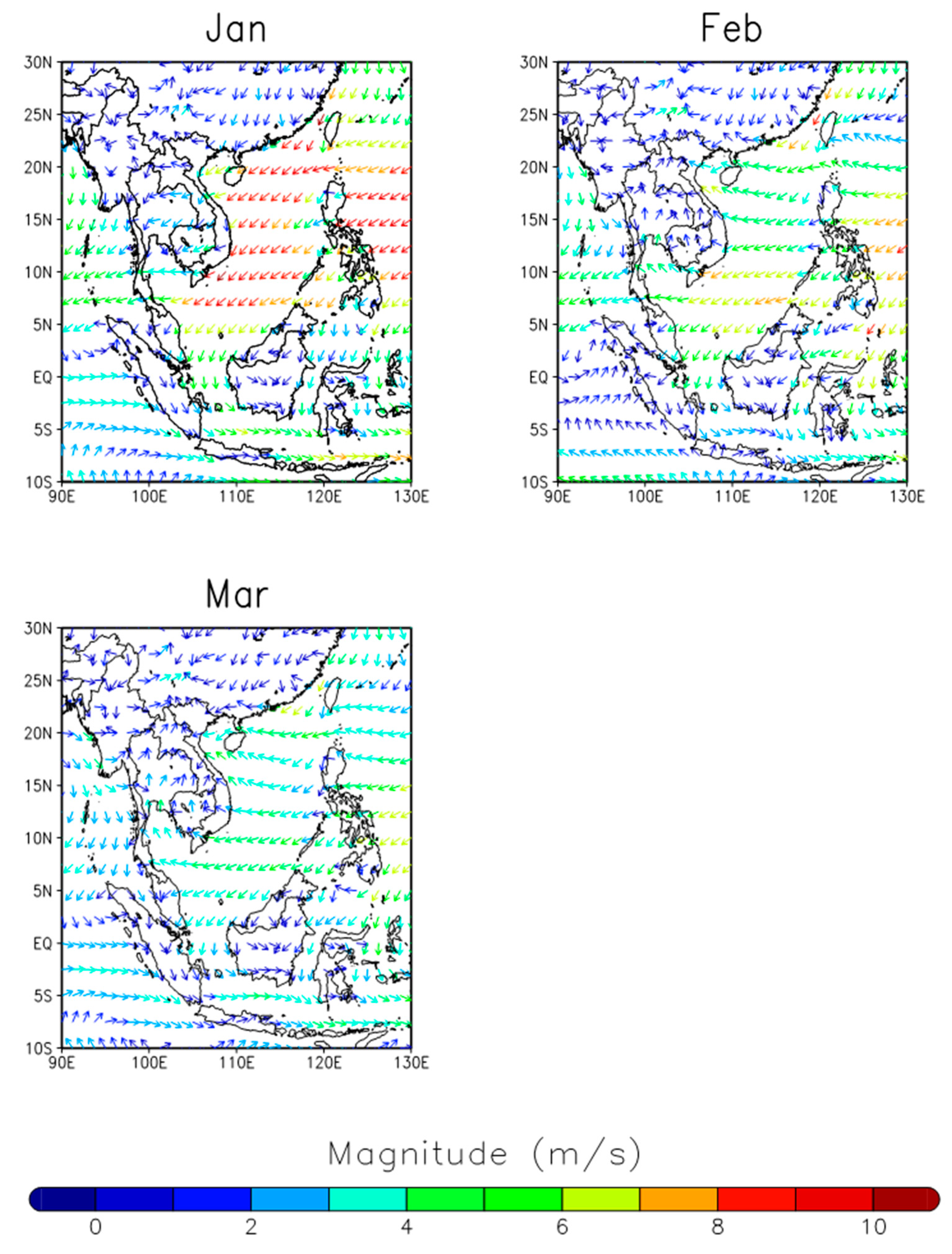
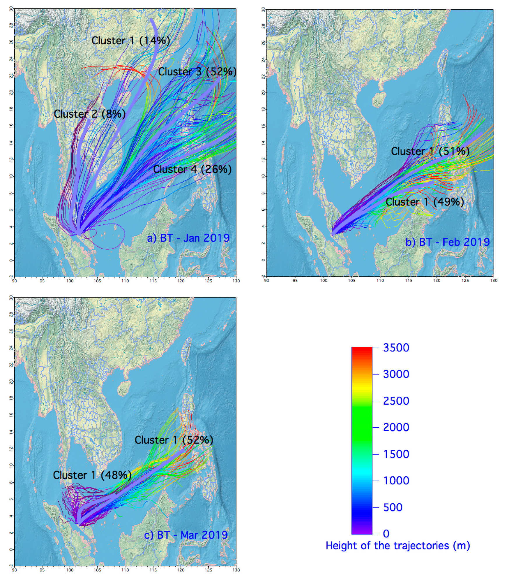
2.2. Local Meteorology and Transport of Air Mass

Kuala Lumpur is located at 56 m above sea level. In the middle of March 2019, the change of ambient temperature was higher compared to January and February, as shown in Figure S1. As shown in Figure S1, the relative humidity inversely changes to ambient temperature. The local meteorology data were taken from Subang Airport (www.wunderground.com, accessed on 18 April 2021) located at about 20 km from Kuala Lumpur. The synoptic level of wind greatly impacts the ambient level of pollutants over Malaysia. As shown in Figure 2, a stronger wind during January was blowing from the South China Sea (north-easterly monsoon) compared to February and March. This strong wind carries more pollutants, as well as water vapor from the ocean [43] to Malaysia, and causes heavy rainfall [44]. The synoptic level wind vector of the assimilated data was downloaded from the ECMWF data repository (European Centre for Medium-Range Weather Forecasts) and plotted using the Grid Analysis and Display System (GrADS) software. As shown in Figure S2, the monthly average of rainfall over the study region was obtained from the ECMWF site. The change in rainfall started to increase from October–November and continued to January, 2019. June, July, and August are relatively drier compared to other periods of the year. Figure 3 shows the monthly cluster of backward trajectories (BTs) constructed using the Hybrid Single-Particle Lagrangian Integrated Trajectory version 4.9 (HYSPLIT 4.9). The BTs were calculated using a set of reanalysis data by NCEP/NCAR (ftp://arlftp.arlhq.noaa.gov/pub/archives/reanalysis, accessed on 18 April 2021) calculated daily on 00, 06, 12, 18 UTC, 500 m as releasing height, 6 h interval, and 120 h as total travel time. Then, the estimated cluster data were plotted in an Igor Pro platform (WaveMetrics, Lake Oswego, OR, USA).

2.3. Air Sampling Procedures

PM_2.5 samples were collected on quartz microfibre filters (203 mm × 254 mm) (Whatman^TM, UK) using a Tisch high-volume sampler (Tisch Environmental, USA). Samples were collected over 24 h (12 a.m. to 12 a.m.) from January to March 2019 at three different locations in Kuala Lumpur which were KKKL, SCA, and DBKL. The filters were prebaked at 500 °C and the initial weight was measured using an electronic microbalance. For each of the locations, two samples were selected in each month randomly with a total of eighteen samples overall. The flowrates of Tisch high-volume sampler for all the samples were recorded and are presented in Table S1 in the Supplementary File. After sample collection, the filters were wrapped with aluminum foil and stored at −25 °C prior to further extraction of PAHs.

2.4. Analysis of OC and EC and Estimation of Secondary Organic Carbon (SOC)

The carbonaceous contents of PM_2.5 were quantified using OC-EC carbon analyzer (Sunset Laboratory Inc., USA), which employs thermal optical reflectance [45] following the IMPROVE_A protocol. The IMPROVE_A temperature defines temperature plateaus for thermally derived carbon fractions as follows: 140 °C for OC1, 280 °C for OC2, 480 °C for OC3, 580 °C for OC4, and OP (splitting of OC and EC) in the presence of helium (He) carrier gas; 580 °C for EC1, 740 °C for EC2, and 840 °C for EC3 in a mixture of 98% He and 2% oxygen carrier gas. From the eight carbon fractions, OC, EC, and total carbon (TC) were calculated as follows in Equations (1)–(3), as described by the Sunset IMPROVE_A protocol and reported by Fujii et al. [46], and Khan et al. [47]:

OC = OC1 + OC2 + OC3 + OC4 + OP

(1)

EC = EC1 + EC2 + EC3 − OP

(2)

TC = OC + EC

(3)

where OP (the amount of pyrolyzed OC) is defined as the carbon content measured after the introduction of O₂ until reflectance returns to its initial value at the start of the analysis.

By using the lowest ratio value of OC to EC (OC/EC), the secondary organic carbon (SOC) concentrations can be estimated. The SOC concentrations were calculated as follows [48,49] in Equation (4):

$$\mathrm{SOC}=\mathrm{OC}-\left[{\left(\frac{\mathrm{OC}}{\mathrm{EC}}\right)}_{\min }\times \mathrm{EC}\right]$$

(4)

where the minimum OC/EC ratio ((OC/EC)_min) is believed to be the value for primary PM_2.5 emission source. Khan et al. [47,50] stated that the lowest value of EC/OC was used to represent the primary combustion source.

2.5. Analysis of Water-Soluble Organic Carbon (WSOC)

A 2 × 2 cm filter (blanks and samples) was cut and placed inside a beaker. Then, 50 mL of ultrapure water was added into the beaker and the sample with the ultrapure water was sonicated for 20 min. After sonication, the mixture was filtered using Whatman filter paper with 100 mm diameter. Then, all the blank and sample solutions were analyzed using Total Organic Carbon Analyzer (TOC-L, Shimadzu, Japan) to determine WSOC concentrations. This methodology was adopted from Thuy et al. [51].

2.6. Extraction Procedures for PAHs in PM_2.5 Samples

Extraction of the PAHs Composition Using Magnetic Nanoparticles

For analysis, the filter paper was cut into one-quarter or half of the filter sample and placed inside a beaker. The exposed filter was extracted using ultrasonic agitation (10 min sonication time) with 25 mL of dichloromethane (DCM) as the solvent. Then, modified magnetic nanoparticles (C₈MNPs) were added immediately into the extraction solution and then sonicated for five minutes. The detailed information of C₈MNPs is described in the supplementary file. Theoretically, the PAHs that were extracted clean up via adsorption on the C₈MNPs. The adsorption efficiency was tested using the recovery analysis of spiking known as the standard of PAHs. After that, with the help of an external magnetic field, the solution was settled down until it was clear. The DCM was thrown away and washed with DCM three times. Next, 200 µL of n-hexane was added to the PAHs adsorbed on C₈MNPs and sonicated for 10 min. PAHs were dissolved in n-hexane. Then, the n-hexane was separated from the magnetic nanoparticles with the help of an external magnetic field, collected, and placed inside a Gas Chromatography (GC) vial. The method reported here is slightly modified from the study published by Tay et al. [52]. Magnetic nanoparticles have been used for many years in the extraction of organic pollutants via the liquid–liquid extraction process [53]. It has been reported that modified MNPs are applicable and feature strong adsorption to multitarget pollutants, e.g., polycyclic aromatic hydrocarbons (PAHs), nitro aromatics, etc. [54].

2.7. Analysis of PAHs Using Gas Chromatography-Flame Ionization Detector (GC-FID)

2.7.1. Preparation of Calibration Standard

A standard mixture of PAHs was used to construct the calibration curves. There are 18 PAHs in the standard mixtures, and each compound eluted at different retention times, following the elution order based on their boiling point.

The standard solution of 0.2 ppm, 0.5 ppm, 1.0 ppm, 2.0 ppm, and 3.0 ppm of PAHs mixtures was prepared. From the standard solution, the calibration curve of peak area against concentration was plotted for each PAH compound. Equation from the calibration curve for each compound was used to determine the concentration of PAHs for all samples.

2.7.2. Determination of PAHs Using GC-FID

The extracted samples were analyzed using the Gas Chromatography-Flame Ionization Detector (GC-FID) (Agilent Technologies 7890A, GC System, USA). A capillary column (HP-5, Agilent, USA) with a length of 30 m, internal diameter (id) 0.320 mm, and thickness 0.25 µm was used. N₂ was used as the make-up gas at the flow rate of around 25 mL/min in GC/FID, while H₂ was used as the carrier gas. The sample was injected in a splitless mode at 270 °C. The GC column temperature was programmed as 40 °C as the initial temperature, followed by temperature increases of 40 to 150 °C at 8 °C min⁻¹ and from 150 to 310 °C at 4 °C min⁻¹ and then the isothermal at 310 °C for 10 min. Then, the peaks were identified for individual PAHs based on the retention time (RT) and the respective boiling point of each compound. Each peak was identified by comparing it with the retention time from the standard solution. The PAHs concentrations were determined using the calibration curve of the standards.

2.8. Quality Assurance and Quality Control (QA/QC)

As for the EC and OC analysis, a set of blank filters were examined, and this determined the thermally derived EC, OC, and other fractions. The EC and OC of the samples were subtracted from the filter blanks. A similar step also followed for GC-FID analysis for PAHs. For EC, OC, and WSOC analysis, concentration of all samples has been subtracted from the blank concentration. In FTIR analysis, baseline correction is done to remove the estimated baseline from the spectrum data and leave only the pure signal and some noise. The extraction of PAHs from PM_2.5 particles was validated through the spiking of 2 ppm of PAHs mixtures at the initial stage of the extraction using MNPs. The recoveries (n = 5) of the PAHs ranged from 61% to 166% for acenaphthene (Ace), 54% to 80% for Benzo (b) fluoranthene, 49% to 70% for Benzo (k) fluoranthene, Benzo (a) pyrene 46% to 61%, and 103% to 118% for Dibenzo (a,h) anthracene. Ace shows a relatively large variation of the recovery (%) from five samples of standard PAHs. There are several studies on environment samples that used the magnetic nanoparticles for the extraction of PAHs and showed excellent recoveries. Shahriman et al. [55] reported that the recovery percentage of PAHs extractions by using MNPs in sludge was in the range of 80.2–111.9%, while for natural water (river, lake, well, paddy, and tap water), the samples were in the range of 83.1–104.9% for Ace, 83.9–102.8% for Flu, 82.5–99.0% for Phe, 81.7–104.8% for Fla, and 83.3–104.5% for Pyr. A study in China recorded that the recoveries of PAHs in rainwater, downstream, upstream, wastewater, and tap water were 87.95%, 82.89%, 85.92%, 78.90%, and 59.23%, respectively [56].

2.9. Data Analysis and Modelling

2.9.1. Statistical Analysis

Statistical analysis was performed using the PAHs and carbonaceous fractions’ results. The initial data analysis, including descriptive statistics, distribution, and correlation, was conducted using IBM Statistic SPSS (Version 25) and Microsoft Excel.

2.9.2. Diagnostic Ratio (DR) and Receptor Modelling

Diagnostic Ratio (DR)

In this study, the sources of the PAHs were estimated using the diagnostic ratio. The PAHs particles can come from many possible sources, as shown in Table S2, as reported in other literature [45,57,58,59,60].

Receptor Modelling

In PCA, the input data were carefully screened and the outliers were cleaned up; data below detection limit and the missing data were replaced with the geometric mean of each variable. To reduce the variability in the concentration, a normalization procedure was followed through the deduction of the concentration from the average value, and then divided with the standard deviation. The rescaled and normalized new database was used for the PCA procedure. Next, the key challenge was to obtain a suitable set of principal component (PC) factors. For this step, we applied several options such as increase or decrease of the number of the factors, threshold of Eigen value, variance (%), and rotation of the PC loadings. An Eigen value is a mathematical term and setting a threshold of Eigen value 1 helps to know the variability to the PC factors. The variance (%) of the PCs may help in knowing the significance of the PCs. To obtain a minimum set of PCs with the largest variability, we applied all the steps described above [24,26,39]. Suitability of the PAHs samples for PCA analysis was tested using the Kaiser–Meyer–Olkin (KMO) test. A large value of KMO (close to one) generally reflected that the data set is suitable to carry out the PCA analysis, while a lower value of KMO indicates less suitability of the data set for PCA analysis. Jamhari et al. [39] suggested that a KMO value of more than 0.6 is required for the suitability of data set in the PCA procedure. The value of KMO in this study is 0.650 which reflects that the dataset of 18 samples is suitable for PCA analysis. Thus, PCA analysis was performed to identify the potential sources of the PAHs samples. To obtain the quantitative contribution of the identified sources, the PCA scores were corrected using absolute principal component scores (APCS) suggested by Thurston and Spengler [40]. Then, the APCS were regressed against the total PAHs concentration.

2.9.3. US EPA Health Risk Modelling

The health risk of PAHs exposure can be estimated via the pathways of ingestion, inhalation, or dermal exposure as suggested by USEPA [61]. However, in this study, inhalation of air particles contaminated with PAHs was considered for health risk assessment, as PM_2.5 is aerodynamically very tiny and can penetrate the human respiratory system to the alveolar level. The Benzo(a)Pyrene equivalent health risk as B[a]Peq was determined using the equation below:

$$\mathrm{B}\left[\mathrm{a}\right]\mathrm{Peq}={\displaystyle \sum }\left({\mathrm{C}}_i\times \mathrm{TEF}\right)$$

(5)

where ${\mathrm{C}}_i$ is the concentration of individual compound in each sample, and TEF indicates toxic equivalency factors, which has a different value for each compound.

The excess lifetime cancer risk (ELCR) in humans and hazard quotient (HQ) can be determined by calculating the lifetime average daily dose (LADD) for carcinogenic and average daily dose for non-carcinogenic exposure of PAHs according to USEPA guidelines [62].

For LADD, the equation is

$$\mathrm{LADD}=\frac{\mathrm{C}\times \mathrm{IR}\times \mathrm{ED}\times \mathrm{EF}}{\mathrm{BW}\times \mathrm{ALT}}$$

(6)

ELCR was calculated as follows:

$$\mathrm{ELCR}=\mathrm{LADD}\times \mathrm{SF}$$

(7)

where C is the concentration in air particles (mg m⁻³), IR is the air inhalation rate, EF is the exposure frequency, ED is the lifetime exposure duration, BW is the body weight, ALT is the averaging lifetime for carcinogens, and SF is the slope factor (mg kg⁻¹ day⁻¹)⁻¹. SF can be determined as

$$\mathrm{SF}=\mathrm{IUR}\times \left[\frac{1}{\mathrm{IR}}\right]\times \mathrm{BW}$$

(8)

where IUR is the inhalation unit risk.

In this study, the health risk assessments are calculated for five age groups, infant, toddler, children, adolescent, and adult, because all these groups are exposed to PAHs pollution. The reference values for all the above constants are shown in Tables S3 and S4 for IUR values.

Lifetime lung cancer risk (LLCR) can be calculated by multiplying the total B[a]Peq with 8.7 × 10⁻⁵ (ngm⁻³)⁻¹.

For non-carcinogenic exposure, the Hazard quotient (HQ) was calculated using ADD and reference dose (${\mathrm{R}}_{\mathrm{f}}\mathrm{D}$). ADD is calculated based on Equation (6).

$$\mathrm{HQ}=\frac{\mathrm{ADD}}{{\mathrm{R}}_{\mathrm{f}}\mathrm{D}}$$

(9)

The value of ${\mathrm{R}}_{\mathrm{f}}\mathrm{D}$ is different for every PAHs compound and has been referred to in Table S5.

3. Results and Discussion

3.1. OC, EC, and SOC

Concentrations of OC1, OC2, OC3, OC4, OP, EC1-OP, EC2, and EC3 are shown in Figure S4a. Concentrations of OC, EC, and TC in each filter sample are shown in Figure S4b and OC to EC ratios for each filter sample are illustrated in Figure S5.

Table 1. Carbonaceous fractions in PM_2.5 from three sites in Kuala Lumpur.

Variables	Sampling Sites	Mean	Min	Max	Standard Deviation
OC (μg/m3)	Overall	6.88	3.12	24.1	4.94
	DBKL	6.99	4.17	13.5	3.30
	SCA	8.73	3.69	24.1	7.64
	KKKL	4.93	3.12	9.33	2.23
EC (μg/m3)	Overall	3.68	1.32	6.82	1.58
	DBKL	4.33	2.76	6.58	1.46
	SCA	3.98	2.53	6.82	1.76
	KKKL	2.73	1.32	4.33	1.25
OC/EC	Overall	1.86	1.24	3.53	0.626
	DBKL	1.60	1.24	2.04	0.343
	SCA	2.01	1.28	3.53	0.820
	KKKL	1.95	1.24	3.04	0.649
SOC (µg/m3)	Overall	2.33	-	15.6	3.61
	DBKL	1.64	-	5.32	1.97
	SCA	3.81	0.13	15.6	5.87
	KKKL	1.56	0.020	3.98	1.43
Soot-EC (µg/m3)	Overall	18	0.28	0.21	0.43
	KKKL	6	0.23	0.21	0.25
	SCA	6	0.30	0.23	0.43
	DBKL	6	0.30	0.21	0.35
Char-EC (µg/m3)	Overall	18	3.40	1.10	6.40
	KKKL	6	2.50	1.10	4.08
	SCA	6	3.68	2.24	6.40
	DBKL	6	4.03	2.49	6.37
WSOC (µg/m3)	Overall	2.73	0.627	9.12	2.17

shows the statistics for all the variables. From Figure S4a, the concentrations of OC2 and OC3 were high in filter samples on 17 March 2019 from SCA and DBKL. OC3 was about 44% of total OC and EC1-OP was about 92% of EC. The OP value was high on 17 March 2019 also at SCA and DBKL with values of 6.40 and 6.37 μg/m³, respectively. From Table 1, the average concentrations of OC and EC are 6.88 ± 4.94 (range from 3.12–24.1) and 3.68 ± 1.58 (range of 1.32–6.82) μg/m³, respectively, with an average OC/EC ratio of 1.86 (range from 1.24–3.53). Fujii et al. [46] reported that the average OC/EC ratio for peatland and background were 36.4 ± 9.08 and 2.99 ± 0.74, respectively, for aerosols emitted from the peatland fire in Riau, Sumatra, Indonesia. This value is greater than the results in the present study. The above study was conducted near a peatland fire area that emits large amounts of organic substances. However, the study site may have its organic pollutants contributed to by domestic activities such as open burning and vehicle emissions. Among the three sampling sites, SCA has the highest concentration of OC with concentrations of 8.73 μg/m³ followed by DBKL and KKKL with concentrations of 6.99 μg/m³ and 4.93 μg/m³, respectively; whereas for EC, DBKL has the highest concentration with a value of 4.33 ± 1.46 μg/m³ followed by SCA (3.98 ± 1.76 μg/m³) and KKKL (2.73 ± 1.25 μg/m³). One-way ANOVA test shows that there is no significant correlation between the value of OC/EC ratio, EC, OC, and TC at the three sites. Several other studies reported EC and OC in PM_2.5 in Malaysia and other Asian countries, as shown in Table S7. Fujii et al. [63] observed 10.7 and 4.11 μg/m³ for OC and EC, respectively, in September of 2013 at a semi-urban site during hazy conditions, in Bandar Baru Bangi in Selangor, Malaysia. During the northeast monsoon, Fujii et al. [64] reported that OC and EC during 2011–2012 in Petaling Jaya, were 5.2 and 3.4 μg/m³, respectively. OC and EC were 2.90 and 1.56 μg/m³, respectively, during the north-easterly monsoon in 2019 from the urban sites in southern Malaysia [65]. Comparing the OC and EC data reported previously in other cities in Malaysia, the levels of OC and EC were relatively high during the north-easterly monsoon.

From Table 1, the average concentration of SOC is 2.33 (range of 0.00 to 15.6) μg/m³, which is 34% of total OC. Consequently, 66% of total OC comes from primary combustion sources. Khan et al. [47] reported that during the southeast dry season (southwest monsoon), estimated SOC was 85% of the total OC and the remaining 15% may have been released from primary combustion sources. In a study in Chiang Mai Province, in northern Thailand, the PSEA reported that the concentration of SOC in Doi Ang Khang (DAK) and Chiang Mai University (CMU) was 9.7 ± 5.0 µg/m³ and 16.7 ± 12.6 µg/m³, respectively [66]. The concentration of SOC in these two study areas is higher compared to Kuala Lumpur because the DAK is located near a source of biomass burning, while CMU is near Chiang Mai city, which is the largest metropolitan city in northern Thailand. Among the three sites, SCA has the highest value of SOC with a concentration of 3.81 μg/m³ followed by DBKL (1.64 μg/m³) and KKKL (1.56 μg/m³). It means that SCA produces more SOC in the atmosphere compared to DBKL and KKKL. The stagnant pollutants and high emission of the local pollutants may contribute to the above change in the SOC concentration. As shown in Table 1, soot-EC and char-EC have been estimated from the EC concentration in PM_2.5 using the method reported by Han et al. [67]. The results from this study show that char-EC is about 12 times greater than soot-EC. Soot-EC potentially emits from vehicle combustion and forest fires while char-EC is released from biomass and coal burning sources [65]. Thus, the PM_2.5 is influenced by biomass and coal combustion sources.

3.2. WSOC

The concentration of WSOC in PM_2.5 (µg/m³) is shown in Table S9. The statistical table for WSOC concentration is shown in Table 1. From this analysis, WSOC mean concentration is 2.73 ± 2.17 (range of 0.63–9.12) µg/m³. This result is higher compared to a previous study in Hanoi, Vietnam that reported the concentration of WSOC in atmospheric nanoparticles as 1.51 (0.90–2.11) µg/m³ and 0.41 (0.51–1.83) µg/m³ in the rainy and dry seasons, respectively [51]. Thuy et al. [51] and Le et al. [68] clearly identified the rainy and dry seasons in Vietnam over the periods of January–August and October–December, respectively.

3.3. Variation of PAHs

Out of 13 measured PAHs, dibenzo(a, h)anthracene (B[h]A) was predominant with a mean concentration of 1.20 ng/m³, followed by indeno(1,2,3-cd)pyrene (I[c]P), benzo [51] perylene (B[g]P), benzo(a)pyrene (B[a]P), benzo(a)anthracene (B[a]A), benzo(k)fluoranthene (B[k]F), acenaphthene (Ace), and benzo(b) fluoranthene (B[b]F) with mean concentrations of 0.95, 0.72, 0.41, 0.39, 0.38, 0.33, and 0.30 ng/m³, respectively, as shown in

Table 2. Summary statistics for the PAHs concentrations (ng/m³) in the PM_2.5 samples.

	Compound	N	Mean	Min	Max	Standard Deviation
Overall	Ace	3	0.33	0.05	0.64	0.30
	Flr	8	0.21	0.04	0.89	0.30
	Ant	10	0.23	0.07	1.06	0.32
	Flt	10	0.16	0.05	0.97	0.29
	Pyr	9	0.19	0.04	0.91	0.29
	B[a]A	5	0.39	0.14	0.96	0.33
	Chr	7	0.21	0.12	0.29	0.06
	B[b]F	12	0.30	0.15	0.38	0.07
	B[k]F	5	0.38	0.29	0.42	0.05
	B[a]P	4	0.41	0.21	0.58	0.15
	I[c]P	2	0.95	0.81	1.08	0.19
	B[h]A	1	1.20	1.20	1.20	-
	B[g]P	1	0.72	0.72	0.72	-
	Total PAHs	13	1.74	0.15	9.94	2.68
DBKL	Flr	1	0.06	0.06	0.06	-
	Ant	2	0.12	0.07	0.16	0.06
	Flt	2	0.09	0.06	0.12	0.04
	Pyr	2	0.06	0.04	0.08	0.02
	B[a]A	1	2.38 × 10−1	2.38 × 10−1	2.38 × 10−1	-
	Chr	1	0.24	0.24	0.24	-
	B[b]F	3	0.34	0.30	0.38	0.04
	B[k]F	1	0.42	0.42	0.42	-
	Total PAHs	3	0.84	0.30	1.46	0.58
SCA	Flr	2	0.06	0.05	0.07	0.01
	Ant	4	0.09	0.07	0.15	0.04
	Flt	4	0.07	0.05	0.13	0.04
	Pyr	3	0.06	0.04	0.09	0.03
	B[a]A	1	0.26	0.26	0.26	-
	Chr	1	0.22	0.22	0.22	-
	B[b]F	3	0.34	0.32	0.37	0.03
	B[k]F	1	0.40	0.40	0.40	-
	B[a]P	1	4.03 × 10−1	4.03 × 10−1	4.03 × 10−1	-
	Total PAHs	4	0.82	0.18	1.37	0.51
KKKL	Ace	3	0.33	0.05	0.64	0.30
	Flr	5	0.30	0.04	0.89	0.37
	Ant	4	0.43	0.07	1.06	0.46
	Flt	4	0.29	0.05	0.97	0.46
	Pyr	4	0.35	0.04	0.91	0.40
	B[a]A	3	0.49	0.14	0.96	0.42
	Chr	5	0.20	0.12	0.29	0.07
	B[b]F	6	0.26	0.15	0.33	0.07
	B[k]F	3	0.35	0.29	0.39	0.06
	B[a]P	3	0.41	0.21	0.58	0.19
	I[c]P	2	0.95	0.81	1.08	0.19
	B[h]A	1	1.20	1.20	1.20	-
	B[g]P	1	0.72	0.72	0.72	-
	Total PAHs	6	2.81	0.15	9.94	3.79

.

Average concentration of total PAHs was 1.74 ± 2.68 (range of 0.15 to 9.94) ng/m³. This value is smaller compared to values in other literature. Concentrations of PM_2.5 for background and peatland fire in Riau, Sumatra, Indonesia were 23.9 ± 2.53 μg/m³ and 7120 ± 3620 μg/m³ as reported by Fujii et al. [46]. Thus, the peatland fire emitted an abundance of PM_2.5 aerosol. Khan et al. [4] reported that the average of the total PAHs at UKM Bangi was 2.79 ng/m³. Sulong et al. [21] described the concentrations of total PAHs in PM_2.5 during the southwest monsoon (January–September), inter-monsoon I (October–November), northeast monsoon (December-March), inter-monsoon II (April-May), and during the haze episode in Kuala Lumpur were 2.51 ± 0.93 ng/m³, 2.87 ± 0.14 ng/m³, 1.37 ± 0.09 ng/m³, 2.20 ± 0.71 ng/m³, and 3.40 ± 0.68 ng/m³, respectively. Jamhari et al. [39] recorded that the total PAHs concentrations in Kuala Lumpur and Petaling Jaya were 2.03 ± 0.69 ng/m³ and 3.56 ± 1.07 ng/m³, respectively. The previously reported PAHs were similar to the PAHs concentration in the present study as the locations are from or nearby Kuala Lumpur. Average concentrations of total PAHs were reported in 2018 at Nan Province and Chiang Mai Province, Thailand with concentrations of 5.21 ng/m³ and 2.02 ng/m³, respectively. The concentrations of PAHs were higher compared to those reported in Kuala Lumpur sites. The reason behind the higher concentration of PAHs at the Nan station is the burning of agricultural residue in the rural area. On the other hand, Chiang Mai is a largest urban area in northern Thailand, and the stations are located near forest burning sources [69].

Out of the three sampling sites, KKKL has the highest average concentration of total PAHs which is 2.81 ± 3.79 ng/m³, followed by DBKL and SCA with mean concentrations of 0.84 ± 0.58 ng/m³ and 0.82 ± 0.51 ng/m³, respectively, as shown in Table 2. The predominant concentrations of PAHs are B[h]A (1.20 ng/m³), I[c]P (0.95 ± 0.19 ng/m³), followed by B[g]P (0.72 ng/m³) at the KKKL site. The trend for mean concentration of PAHs in KKKL is B[h]A > I[c]P > B[g]P > B[a]A > Ant > B[a]P > Pyr > B[k]F > Ace > Flr > Flt > B[b]F > Chr. For DBKL, eight PAHs were detected with B[k]F (0.42 ng/m³) as the largest mean concentration, followed by B[b]F 0.34 ± 0.04 ng/m³, and Chr 0.24 ng/m³. The trend for the mean concentration of PAHs in DBKL is B[k]F > B[b]F > Chr > B[a]A > Ant > Flt > Flr > Pyr. As for SCA, the highest mean concentration is B[a]P and B[k]F (4.03 × 10⁻¹ ng/m³ and 0.40 ng/m³, respectively, followed by B[b]F with mean concentration of 0.34 ± 0.03 ng/m³. Nine PAHs were detected in SCA. The trend for the mean concentration of PAHs in SCA is B[a]P > B[k]F > B[b]F > B[a]A > Chr > Ant > Flt > Flr > Pyr. As for the comparison, total PAHs were highest at the KKKL site compared to other two sampling sites in Kuala Lumpur. This site is located at a medical center and is influenced by the high frequency of traffic due to the presence of an educational institute.

3.4. Identification of Possible Sources

3.4.1. Diagnostic Ratio (DR)

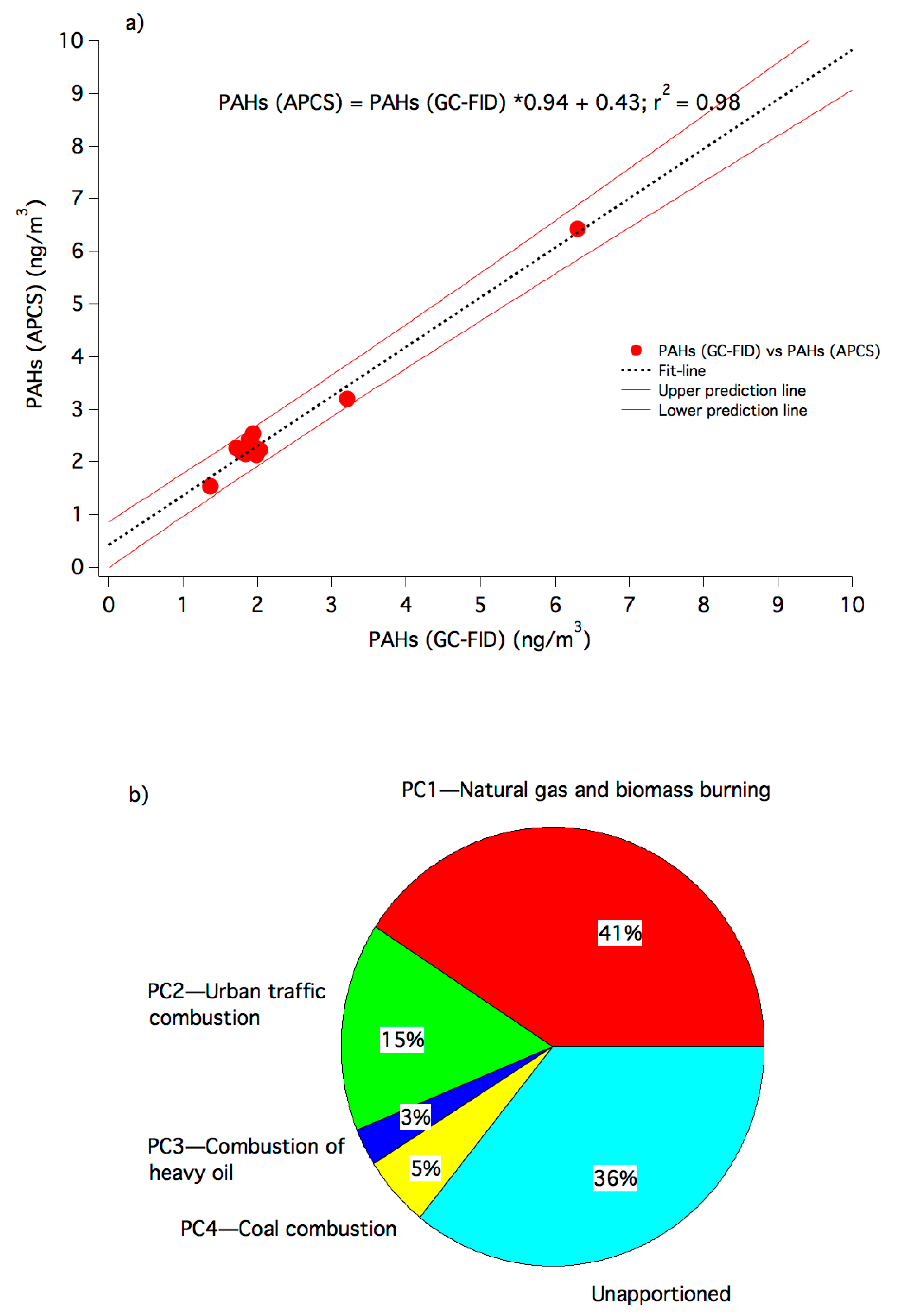
Application of Ant/(Ant + Phe) was not possible because no phenanthrene was detected in the samples. From Table S2, the mean ratio of Flt to (Flt + Pyr) is 0.5459. This ratio value suggests that the PAHs have been released from coal, grass, and wood burning, as reported by Yunker et al. [59] and De La Torre-Roche et al. [45]. Similarly, the ratio of B[a]A to (B[a]A + Chr) is 0.58, which implies that the PAHs were emitted from wood burning activities, as reported by Akyüz and Çabuk [60], Manoli et al. [58], and Yunker et al. [59]. The ratio of I[c]P to (I[c]P + B[g]P) obtained was 0.60. Brändli et al. [57] and Yunker et al. [59] suggested that these PAHs come from the emission of coal, wood, and grass burning, as well as from diesel. From the ratio of B[a]P/B[g]P, the value of 0.82 was emitted from traffic as proposed by Brändli et al. [57] and Yunker et al. [59]. The PAHs are estimated to come mainly from coal, grass, and wood burning activities, as well as from traffic emission. The high density of traffic in the sampling site is a potential cause in this regard and the wind speed and flow brought the PAHs from the coal and open burning near the sampling site.

3.4.2. PCA-MLR

PCA factor loadings obtained via the varimax rotation are shown in

Table 3. The factor loadings of PAHs after PCA varimax rotation at the study areas.

Variables	Factor 1	Factor 2	Factor 3	Factor 4
Fluorene	0.955	0.049	0.058	0.271
Anthracene	0.970	0.043	0.010	0.202
Fluoranthene	0.976	0.052	0.081	−0.080
Pyrene	0.977	0.031	0.025	0.186
Benzo(a)anthracene	0.957	0.258	0.036	−0.013
Chrysene	0.196	0.271	0.314	0.884
Benzo(b)fluoranthene	0.049	0.173	0.954	0.239
Benzo(k)fluoranthene	0.037	0.952	0.179	0.213
Benzo(a)pyrene	0.757	0.629	0.066	0.093
Eigen values	5.787	1.824	0.803	0.462
Variance (%)	64.301	20.267	8.926	5.133
Cumulative (%)	64.301	84.568	93.494	98.627
Sources of the pollutants	Natural gas and biomass burning	Urban traffic combustion	Combustion of heavy oil	Coal combustion

. The PCA analysis arranged the dataset of PAHs into four principal components (PCs) that control 98.63% of the data variance in Kuala Lumpur. Factor 1 (64.3% of the total variance) was highly loaded on Flu, Ant, Flt, Pyr, B[a]A and B[a]P, suggesting that the emissions are from natural gas and coal burning sources [25,70,71]. Ant, Pyr, and B[a]A are typical indicators of wood combustion while B[a]P is from the emission of coal combustion [26]. Flt, Pyr, and B[a]A were applied as the tracers for the emission from natural gas [24,39]. Sulong et al. [21] reported that Flu, Ant, Flt, and Pyr are emissions from natural gas and biomass burning. B[a]P is a specific marker for vehicle and gasoline emissions [21,25,26,39]. Thus, Factor 1 has been classified as natural gas, coal, and biomass burning. Factor 2 (20.27% of the total variance) was highly loaded with B[k]F and B[a]P. The presence of B[k]F to the factor profile was reported earlier as the tracer of diesel vehicles [32]. Similarly, B[a]P has been widely applied in literature as a specific marker for vehicle and gasoline emissions [21,25,26,39]. Therefore, Factor 2 was identified as the urban traffic combustion source. Factor 3 (8.93% of the total variance) was the third most common factor profile. B[b]F as a high molecular weight of PAHs was the potential variable in Factor 3. B[b]F emits from the combustion of heavy oil, as reported by Khan et al. [4] and Harrison et al. [25]. Factor 4 (5.13% of total variance) appeared as the fourth most significant factor profile. Chr was the most dominant tracer in Factor 4. Chr has been recognized in several studies as a marker of coal combustion [26,32]. Thus, Factor 4 has been classified as the coal combustion source.

The air pollutants in Malaysia during the northeasterly monsoon may be influenced severely by the local anthropogenic emission, air mass transporting from the South China Sea, and the polluted aged air mass from East Asia, as reported by Farren et al. [15]. Metro Manila also experienced a spike of smoke aerosol from the long-range maritime continent as identified by Braun et al. [72]. Biomass burning potentially occurred in the Indochina [73,74] and East Asian regions [75] and was reported as a predominant source of PAHs in PM_2.5 [76]. From the synoptic scale wind vector using the u- and v-components at 10 m above sea level (asl) by each month, as shown in Figure 2, the wind blew from the South China Sea towards the Malaysian region. As reported by Khan et al. [44] during the north-east monsoon, strong winds transporting from the South China Sea region causes rainfall and influences the air quality due to the polluted air stream from the Indochina region. Back track trajectory of air mass was plotted to further observe the direction of wind blown to the monitoring site. Backward trajectory (BT) using HYSPLIT model as shown in Figure 3 depicts that the northeast monsoon wind arrives over three months (Figure 3a—January, Figure 3b—February and Figure 3c—March) towards the monitoring stations. Cluster analysis of BTs for an entire month provides very consistent and reliable pathways of air mass as compared to the trajectories calculated limited to a few days. Considering Figure 3a on January, there are four main clusters of back trajectories in which cluster 1 is blown from the Indochina region at about 14%, cluster 2 shows 8% blowing from a similar Indochina region, cluster 3 shows 52% both from the South China Sea region, and cluster 4 shows 26% from the Philippines region. Figure 3b on February and Figure 3c on March show a similar pattern where there are two main clusters of back trajectories in which both clusters were blown from the South China Sea region. Therefore, the source of transboundary pollutants may also be contributed from the activities in the South China Sea. However, the discussion on the transport of air mass does not consider the deposition or dispersion of pollutants over the boundary layer (BL).

The quantitative source apportionment of PAHs was determined using the APCS-MLR procedure. The regression plot between PAHs from GC-FID and PAHs as predicted by APCS shows a significant correlation (R² = 0.98). From Figure 4, the identified factors were emission from natural gas and biomass burning (Factor 1), urban traffic combustion (Factor 2), combustion of heavy oil (Factor 3), and coal combustion (Factor 4). These four factors contributed 30% (Factor 1), 5% (Factor 2), 3% (Factor 3), and 5% (Factor 4), respectively, leaving 57% of the PAHs concentration as undefined. The percentage of undefined PAHs is higher because some of the variables were excluded, as the data are ≤30% from overall variables and many other PAHs were not determined. There may be some uncertainties associated with the results by PCA-APCS due to the limited number of 18 samples. However, the suitability test by KMO suggests that the dataset is suitable for PCA analysis.

3.5. Human Exposure to PAH

3.5.1. Toxicity Risk

BaP_eq was estimated via multiplying the PAH concentration with the respective TEF value to estimate the toxicity of the compound by comparing them with the concentration of B[a]P. Table S9 shows that there is no BaPeq concentration that is higher than the B[a]P compound (1.63 ng/m³). B[h]A also gives a relatively high concentration of BaPeq, which is 1.20 ng/m³. The total concentration of BaP_eq is 3.82 ng/m³, with the average of 0.29 (range of 0.001–1.62) ng/m³. This value is almost the same as that obtained in the study by Sulong et al. [21], who reported that the total BaP_eq concentration in Kuala Lumpur during different monsoon seasons and haze episodes was 0.266 ng/m³. Liu et al. [9] reported that the mean concentration of total BaPeq in Guangzhou China was 6.69 (range of 0.96–22.46 ng/m³), which is much higher compared to the result in this study. This is due to the rapid industrialization and insufficient emission control in the sampling area, Guangzhou China. BaPeq (ng/m³) was observed in China, Japan, South Korea, Vietnam, and India with the value of 7.79 (range of 0.49–34.8), 0.288 (0.09–0.71), 1.21 (0.61–2.66), 4.44 (1.26–10.6), and 5.79 (0.95–19.0) ng/m³, respectively [36]. The lifetime lung cancer risk (LLCR) can be estimated from the total BaPeq,. Zhang et al. [77] stated that LLCR < 1.0 × 10⁻⁶, 1.0 × 10⁻⁶ < LLCR < 1.0 × 10⁻⁴, 1.0 × 10⁻⁴ < LLCR < 1.0 × 10⁻³, 1.0 × 10⁻³ < LLCR < 1.0 × 10⁻¹, and LLCR > 1.0 × 10⁻¹ as very low cancer risk, low risk, moderate risk, high risk, and very high risk, respectively. In this study, the calculated value is 3.32 × 10⁻⁴, and is classified as moderate risk.

3.5.2. Carcinogenic Exposure

Lifetime Average Daily Dose

Carcinogenic lifetime average daily dose (LADD) concentrations for infant, toddler, children, adolescent, and adult are shown in Table S10. The concentrations follow the order of adult > toddler > adolescent > children > infant. Adult has the highest concentration which is 1.29 × 10⁻⁷ (range of 1.09 × 10⁻⁸ to 7.33 × 10⁻⁷) mg/kg day followed by toddler, adolescent, children, and infant with values of 7.17 × 10⁻⁸ (range of 6.08 × 10⁻⁹ to 4.08 × 10⁻⁷), 5.92 × 10⁻⁸ (range of 5.02 × 10⁻⁹ to 3.37 × 10⁻⁷), 5.51 × 10⁻⁸ (range of 4.67 × 10⁻⁹ to 3.14 × 10⁻⁷) and 1.84 × 10⁻⁸ (range of 1.56 × 10⁻⁹ to 1.05 × 10⁻⁷) mg/kg day, respectively. From Table S10, B[h]A has the highest concentration compared to other compounds in all age groups.

Excess Lifetime Cancer Risk (ELCR)

From Table S12a, B[h]A in all age groups has the highest ELCR value compared to other compounds, followed by B[a]P and I[c]P. These compounds have high molecular weight that has high stability and classified as carcinogenic. Mean concentration of the PAHs for all age groups followed the order of B[h]A > B[a]P > I[c]P > B[a]A > B[k]F > B[b]F > B[g]P > Ant > Chr > Ace > Flr > Pyr > Flt. Table ELCR shows that the pattern of the PAHs inhalation exposure is adult > children > adolescent > toddler > infant. Sulong et al. [21] described that the cancer risk in their study followed the order of adult > toddler > adolescent > children > infant. The result for adults and children are similar compared to the current study in which adult has the highest value and infant has the lowest value of incremental lifetime cancer risk (ILCR). Jamhari et al. [39] also reported that the adult group has the highest ILCR value and infant has the lowest value of ILCR among the age groups. The adult group has the highest health risk compared to others because it is exposed to the carcinogen for a long period of time compared to other age groups. This is possibly due to the longer time exposure as the concentration of carcinogenic element can accumulate in the body over an extended lifetime. However, the estimated cancer risk that has been calculated was considered insignificant and safe since the values are less than 1 × 10⁻⁶.

Table S12b shows that the adult group has the highest values of ELCR whereas the infant group has the lowest values of ELCR for each sampling site. For DBKL, B[k]F has the highest ELCR values followed by B[b]F, B[a]A, and Chr for each age group. As for SCA, for all age groups, B[a]P has the highest ELCR values, followed by B[k]F, B[b]F, and B[a]A, while for KKKL, B[h]A has the highest ELCR value followed by B[a]P, B[a]A and I[c]P for each age group.

3.5.3. Non-Carcinogenic Exposure

Average Daily Dose (ADD) for Non-Carcinogenic Exposure

Table S11 shows the ADD for non-cancer risk for infant, toddler, children, adolescent, and adult. The ADD for average total PAHs follows the order of infant > toddler > adolescent > children > adult. Infant has the highest average of total PAHs while adult has the lowest ADD with a value of 1.34 × 10⁻⁶ (range of 1.14 × 10⁻⁷ to 7.67 × 10⁻⁶) and 3.91 × 10⁻⁷ (range of 3.32 × 10⁻⁸ to 2.23 × 10⁻⁶) mg/ kg day, respectively.

Hazard Quotient (HQ) and Hazard Index (HI)

For non-carcinogenic risk detection, Hazard Quotient (HQ) and Hazard Index (HI) are used. HQ is obtained by dividing ADD with R_fD values, while HI is estimated by the summation of HQ values for every age group. As shown in Table S13a, the trend for average total PAHs HQ is infant > toddler > adolescent > children > adult. Infant has the highest HQ value which is 3.92 × 10⁻⁴, followed by toddler, adolescent, children, and adult which have the HQ values of 3.05 × 10⁻⁴, 2.10 × 10⁻⁴, 1.96 × 10⁻⁴, and 1.14 × 10⁻⁴, respectively. Compared to other compounds, HQ for B[a]P for all age groups is the highest, with a value of × 10⁻³ to × 10⁻⁴. Khpalwak et al. [26] observed the HQ via inhalation route for road and aerial dust from the cities of Kabul and Jalalabad, Afghanistan. HQ was estimated from three types of air particles such as road-dust Kabul, road-dust Jalalabad, and aerial-dust Jalalabad at 2.99 × 10⁻⁹ (children) and 5.12 × 10⁻⁹ (adult), 1.42 × 10⁻⁹ (children) and 2.44 × 10⁻⁹ (adult), and 2.36 × 10⁻⁹ (children) and 1.38 × 10⁻⁹ (children), respectively. From Table S13b, the trends of HQ for all sampling sites are the same, which is infant > toddler > adolescent > children > adult. KKKL has the highest HQ of mean total PAHs in KKKL followed by SCA and DBKL. For all age groups, HQ for B[a]P is the highest compared to other compounds in both KKKL and SCA, while for DBKL, the highest HQ is Flt.

From the current study, HI for infant is the highest with a value of 0.0043, followed by toddler, adolescent, children, and adult with values of 0.0034, 0.0023, 0.0022, and 0.0013, respectively. The trend is also similar to the trend of HQ for each age group. Our results show that none of the age groups are at risk of HI >1. All age groups show HI values of 10⁻³, which is lower than one (<1). In addition, for every age group, DBKL HI values of × 10⁻⁶ which is lower than those of SCA and KKKL. Thus, non-carcinogenic health effect is less prominent at the study areas.

4. Conclusions

This study determined the concentrations of carbonaceous fractions and PAHs in Kuala Lumpur. The concentrations of OC₁, OC₂, OC₃, OC₄, OP, EC_1, EC₂, and EC₃ were determined by using IMPROVE_A protocol, and then the concentration of SOC was estimated. Of the total OC, 34% is produced in the atmosphere as SOC, while 66% of the total OC comes from primary sources. The average concentration of WSOC was 2.73 ± 2.17 (range of 0.63–9.12) µg/m³. The average concentration of total PAHs in this study was 1.74 ± 2.68 ng/m³. The estimated PAHs particles mainly came from natural gas and biomass burning (coal, grass, and wood burning) and fuel combustion. From the concentrations of PAHs obtained, health risk assessment for age groups of infants, toddler, children, adolescent, and adult were also conducted. Adult has the highest ELCR, whereas infant has the lowest ELCR. However, carcinogenic risks were insignificant because the values were not in the range of 1.00 × 10⁻⁶ to 1.00 × 10⁻⁴. For non-carcinogenic risk, infant has the highest HQ value followed by toddler, adolescent, children, and adult. HI values for all age groups were less than one (<1), which means that no substantial non-cancerous risk is present. Although the health risk assessment that has been done shows no significant health risk for both carcinogenic and non-carcinogenic risk, precautionary measures must be taken to reduce PAHs exposure. To better elucidate potential PAHs emission sources, the use of multivariate source apportionment modeling, e.g., PMF with long-term monitoring data, would be needed. In future studies, we will consider long-term sampling and the breathing zone or level for the PM_2.5 sampling to avoid the bias in risk analysis. To reduce emission from biomass burning and vehicle combustion, the government should take action against those who carry out open burning or uncontrolled biomass burning, and encourage the public to use public transport rather than drive their own vehicles. Thus, the representative results of EC, OC, WSOC, and PAHs in PM_2.5 for Kuala Lumpur will have potential implications of knowing the air quality, emitting sources, and health impact in the study areas.

References

1. Brauer, M.; Freedman, G.; Frostad, J.; van Donkelaar, A.; Martin, R.V.; Dentener, F.; Dingenen, R.v.; Estep, K.; Amini, H.; Apte, J.S.; et al. Ambient Air Pollution Exposure Estimation for the Global Burden of Disease 2013. Environ. Sci. Technol. 2016, 50, 79–88. [Google Scholar] [CrossRef]
2. Cohen, A.J.; Brauer, M.; Burnett, R.; Anderson, H.R.; Frostad, J.; Estep, K.; Balakrishnan, K.; Brunekreef, B.; Dandona, L.; Dandona, R.; et al. Estimates and 25-year trends of the global burden of disease attributable to ambient air pollution: An analysis of data from the Global Burden of Diseases Study 2015. Lancet 2017, 389, 1907–1918. [Google Scholar] [CrossRef] [Green Version]
3. WHO. World Health Organization. Global Urban Ambient Air Pollution Database (Update 2016); World Health Organization: Geneva, Switzerland, 2016. [Google Scholar]
4. Khan, M.F.; Latif, M.T.; Lim, C.H.; Amil, N.; Jaafar, S.A.; Dominick, D.; Nadzir, M.S.M.; Sahani, M.; Tahir, N.M. Seasonal effect and source apportionment of polycyclic aromatic hydrocarbons in PM2.5. Atmos. Environ. 2015, 106, 178–190. [Google Scholar] [CrossRef]
5. Liu, X.; Schnelle-Kreis, J.; Schloter-Hai, B.; Ma, L.; Tai, P.; Cao, X.; Yu, C.; Adam, T.; Zimmermann, R. Analysis of PAHs Associated with PM10 and PM2.5 from Different Districts in Nanjing. Aerosol Air Qual. Res. 2019, 19, 2294–2307. [Google Scholar] [CrossRef] [Green Version]
6. Omar, N.Y.M.; Mon, T.C.; Rahman, N.A.; Abas, M.R.B. Distributions and health risks of polycyclic aromatic hydrocarbons (PAHs) in atmospheric aerosols of Kuala Lumpur, Malaysia. Sci. Total Environ. 2006, 369, 76–81. [Google Scholar] [CrossRef] [PubMed]
7. Zhang, N.; Cao, J.; Li, L.; Ho, S.S.H.; Wang, Q.; Zhu, C.; Wang, L. Characteristics and source identification of polycyclic aromatic hydrocarbons and n-alkanes in PM2.5 in Xiamen. Aerosol Air Qual. Res. 2018, 18, 1673–1683. [Google Scholar] [CrossRef]
8. WHO. World Health Organization. Particulate Matter, Chapter 7.3; WHO Regional Publications: Copenhagen, Denmark, 2000. [Google Scholar]
9. Liu, J.; Man, R.; Ma, S.; Li, J.; Wu, Q.; Peng, J. Atmospheric levels and health risk of polycyclic aromatic hydrocarbons (PAHs) bound to PM2.5 in Guangzhou, China. Mar. Pollut. Bull. 2015, 100, 134–143. [Google Scholar] [CrossRef] [PubMed]
10. Seinfield, J.H.; Pandis, S.N. Atmospheric Chemistry and Physics: From Air Pollution to Climate Change; John Wiley & Sons: Hoboken, NJ, USA, 2016. [Google Scholar]
11. Wang, J.; Ogawa, S. Effects of meteorological conditions on PM2.5 concentrations in Nagasaki, Japan. Int. J. Environ. Res. Public Health 2015, 12, 9089–9101. [Google Scholar] [CrossRef]
12. Dominick, D.; Latif, M.T.; Juneng, L.; Khan, M.F.; Amil, N.; Mead, M.I.; Nadzir, M.S.M.; Moi, P.S.; Samah, A.A.; Ashfold, M.J. Characterisation of particle mass and number concentration on the east coast of the Malaysian Peninsula during the northeast monsoon. Atmos. Environ. 2015, 117, 187–199. [Google Scholar] [CrossRef]
13. Rahim, H.A.; Khan, M.F.; Ibrahim, Z.F.; Shoaib, A.; Suradi, H.; Mohyeddin, N.; Samah, A.A.; Yusoff, S. Coastal meteorology on the dispersion of air particles at the Bachok GAW Station. Sci. Total Environ. 2021, 782, 146783. [Google Scholar] [CrossRef] [PubMed]
14. Mohyeddin, N.; Samah, A.A.; Chenoli, S.N.; Ashfold, M.J.; Mead, M.I.; Oram, D.; Latif, M.T.; Sivaprasad, P.; Mohd Nor, M.F.F. The effects of synoptic and local meteorological condition on CO2, CH4, PM10 and PM2.5 at Bachok Marine Research Station (BMRS) in Peninsular Malaysia. Meteorol. Atmos. Phys. 2020, 132, 845–868. [Google Scholar] [CrossRef]
15. Farren, N.J.; Dunmore, R.E.; Mead, M.I.; Nadzir, M.S.M.; Samah, A.A.; Phang, S.-M.; Bandy, B.J.; Sturges, W.T.; Hamilton, J.F. Chemical characterisation of water-soluble ions in atmospheric particulate matter on the east coast of Peninsular Malaysia. Atmos. Chem. Phys. 2019, 19, 1537–1553. [Google Scholar] [CrossRef] [Green Version]
16. Khan, M.F.; Latif, M.T.; Amil, N.; Juneng, L.; Mohamad, N.; Nadzir, M.S.M.; Hoque, H.M.S. Characterization and source apportionment of particle number concentration at a semi-urban tropical environment. Environ. Sci. Pollut. Res. Int. 2015, 22, 13111–13126. [Google Scholar] [CrossRef] [PubMed]
17. Wu, C.; Yu, J.Z. Determination of primary combustion source organic carbon-to-elemental carbon (OC/EC) ratio using ambient OC and EC measurements: Secondary OC-EC correlation minimization method. Atmos. Chem. Phys. 2016, 16, 5453–5465. [Google Scholar] [CrossRef] [Green Version]
18. Rajput, P.; Sarin, M.; Kundu, S.S. Atmospheric particulate matter (PM2.5), EC, OC, WSOC and PAHs from NE–Himalaya: Abundances and chemical characteristics. Atmos. Pollut. Res. 2013, 4, 214–221. [Google Scholar] [CrossRef] [Green Version]
19. Zhang, H.; Ying, Q. Secondary organic aerosol from polycyclic aromatic hydrocarbons in Southeast Texas. Atmos. Environ. 2012, 55, 279–287. [Google Scholar] [CrossRef]
20. Ding, X.; Wang, X.-M.; Gao, B.; Fu, X.-X.; He, Q.-F.; Zhao, X.-Y.; Yu, J.-Z.; Zheng, M. Tracer-based estimation of secondary organic carbon in the Pearl River Delta, south China. J. Geophys. Res. 2012, 117. [Google Scholar] [CrossRef]
21. Sulong, N.A.; Latif, M.T.; Sahani, M.; Khan, M.F.; Fadzil, M.F.; Tahir, N.M.; Mohamad, N.; Sakai, N.; Fujii, Y.; Othman, M. Distribution, sources and potential health risks of polycyclic aromatic hydrocarbons (PAHs) in PM2.5 collected during different monsoon seasons and haze episode in Kuala Lumpur. Chemosphere 2019, 219, 1–14. [Google Scholar] [CrossRef]
22. Zhang, Y.; Tao, S.; Shen, H.; Ma, J. Inhalation exposure to ambient polycyclic aromatic hydrocarbons and lung cancer risk of Chinese population. Proc. Natl. Acad. Sci. USA 2009, 106, 21063–21067. [Google Scholar] [CrossRef] [PubMed] [Green Version]
23. USEPA United States Environmental Protection Agency. Risk Assessment Guidance for Superfund: Volume 1, Human Health Evaluation Manual (Part D, Standardized Planning, Reporting, and Review of Superfund Risk Assessments); Office of Emergency and Remedial Response U.S. Environmental Protection Agency: Washington, DC, USA, 2001.
24. Chiu, T.R.; Khan, M.F.; Latif, M.T.; Mohd Nadzir, M.S.; Abdul Hamid, H.H.; Yusoff, H.; Mohd Ali, M. Distribution of Polycyclic Aromatic Hydrocarbons (PAHs) in Surface Sediments of Langkawi Island, Malaysia. Sains Malays. 2018, 47, 871–882. [Google Scholar] [CrossRef]
25. Harrison, R.M.; Smith, D.J.T.; Luhana, L. Source Apportionment of Atmospheric Polycyclic Aromatic Hydrocarbons Collected from an Urban Location in Birmingham, U.K. Environ. Sci. Technol. 1996, 30, 825–832. [Google Scholar] [CrossRef]
26. Khpalwak, W.; Jadoon, W.A.; Abdel-dayem, S.M.; Sakugawa, H. Polycyclic aromatic hydrocarbons in urban road dust, Afghanistan: Implications for human health. Chemosphere 2019, 218, 517–526. [Google Scholar] [CrossRef] [PubMed]
27. Yu, Q.; Yang, W.; Zhu, M.; Gao, B.; Li, S.; Li, G.; Fang, H.; Zhou, H.; Zhang, H.; Wu, Z.; et al. Ambient PM2.5-bound polycyclic aromatic hydrocarbons (PAHs) in rural Beijing: Unabated with enhanced temporary emission control during the 2014 APEC summit and largely aggravated after the start of wintertime heating. Environ. Pollut. 2018, 238, 532–542. [Google Scholar] [CrossRef]
28. Peltonen, K.; Kuljukka, T. Air sampling and analysis of polycyclic aromatic hydrocarbons. J. Chromatogr. A 1995, 710, 93–108. [Google Scholar] [CrossRef]
29. Gao, B.; Yu, J.-Z.; Li, S.-X.; Ding, X.; He, Q.-F.; Wang, X.-M. Roadside and rooftop measurements of polycyclic aromatic hydrocarbons in PM2.5 in urban Guangzhou: Evaluation of vehicular and regional combustion source contributions. Atmos. Environ. 2011, 45, 7184–7191. [Google Scholar] [CrossRef]
30. Pongpiachan, S.; Tipmanee, D.; Khumsup, C.; Kittikoon, I.; Hirunyatrakul, P. Assessing risks to adults and preschool children posed by PM2.5-bound polycyclic aromatic hydrocarbons (PAHs) during a biomass burning episode in Northern Thailand. Sci. Total Environ. 2015, 508, 435–444. [Google Scholar] [CrossRef] [PubMed]
31. Wang, J.; Geng, N.B.; Xu, Y.F.; Zhang, W.D.; Tang, X.Y.; Zhang, R.Q. PAHs in PM2.5 in Zhengzhou: Concentration, carcinogenic risk analysis, and source apportionment. Environ. Monit. Assess. 2014, 186, 7461–7473. [Google Scholar] [CrossRef]
32. Liu, Y.; Chen, L.; Huang, Q.-h.; Li, W.-y.; Tang, Y.-j.; Zhao, J.-f. Source apportionment of polycyclic aromatic hydrocarbons (PAHs) in surface sediments of the Huangpu River, Shanghai, China. Sci. Total Environ. 2009, 407, 2931–2938. [Google Scholar] [CrossRef]
33. Goel, A.; Ola, D.; Veetil, A.V. Burden of disease for workers attributable to exposure through inhalation of PPAHs in RSPM from cooking fumes. Environ. Sci. Pollut. Res. 2019, 26, 8885–8894. [Google Scholar] [CrossRef] [PubMed]
34. Li, H.; Li, H.; Zhang, L.; Cheng, M.; Guo, L.; He, Q.; Wang, X.; Wang, Y. High cancer risk from inhalation exposure to PAHs in Fenhe Plain in winter: A particulate size distribution-based study. Atmos. Environ. 2019, 216, 116924. [Google Scholar] [CrossRef]
35. Sarkar, S.; Khillare, P. Profile of PAHs in the inhalable particulate fraction: Source apportionment and associated health risks in a tropical megacity. Environ. Monit. Assess. 2013, 185, 1199–1213. [Google Scholar] [CrossRef]
36. Hong, W.-J.; Jia, H.; Ma, W.-L.; Sinha, R.K.; Moon, H.-B.; Nakata, H.; Minh, N.H.; Chi, K.H.; Li, W.-L.; Kannan, K. Distribution, fate, inhalation exposure and lung cancer risk of atmospheric polycyclic aromatic hydrocarbons in some Asian countries. Environ. Sci. Technol. 2016, 50, 7163–7174. [Google Scholar] [CrossRef] [PubMed]
37. Khan, M.F.; Latif, M.T.; Saw, W.H.; Amil, N.; Nadzir, M.S.M.; Sahani, M.; Tahir, N.M.; Chung, J.X. Fine particulate matter in the tropical environment: Monsoonal effects, source apportionment, and health risk assessment. Atmos. Chem. Phys. 2016, 16, 597–617. [Google Scholar] [CrossRef] [Green Version]
38. Hopke, P.K. Review of receptor modeling methods for source apportionment. J. Air Waste Manag. Assoc. 2016, 66, 237–259. [Google Scholar] [CrossRef] [PubMed]
39. Jamhari, A.A.; Sahani, M.; Latif, M.T.; Chan, K.M.; Tan, H.S.; Khan, M.F.; Tahir, N.M. Concentration and source identification of polycyclic aromatic hydrocarbons (PAHs) in PM10 of urban, industrial and semi-urban areas in Malaysia. Atmos. Environ. 2014, 86, 16–27. [Google Scholar] [CrossRef]
40. Thurston, G.D.; Spengler, J.D. A quantitative assessment of source contributions to inhalable particulate matter pollution in metropolitan Boston. Atmos. Environ. 1985, 19, 9–25. [Google Scholar] [CrossRef]
41. Alias, N.F.; Khan, M.F.; Sairi, N.A.; Zain, S.M.; Suradi, H.; Rahim, H.A.; Banerjee, T.; Bari, M.A.; Othman, M.; Latif, M.T. Characteristics, Emission Sources, and Risk Factors of Heavy Metals in PM2.5 from Southern Malaysia. ACS Earth Space Chem. 2020, 4, 1309–1323. [Google Scholar] [CrossRef]
42. Worldometers. Malaysia Population. Available online: https://www.worldometers.info/world-population/malaysia-population/ (accessed on 31 December 2019).
43. ChooChuay, C.; Pongpiachan, S.; Tipmanee, D.; Suttinun, O.; Deelaman, W.; Wang, Q.; Xing, L.; Li, G.; Han, Y.; Palakun, J. Impacts of PM2.5 sources on variations in particulate chemical compounds in ambient air of Bangkok, Thailand. Atmos. Pollut. Res. 2020, 11, 1657–1667. [Google Scholar] [CrossRef]
44. Khan, M.F.; Maulud, K.N.A.; Latif, M.T.; Chung, J.X.; Amil, N.; Alias, A.; Nadzir, M.S.M.; Sahani, M.; Mohammad, M.; Jahaya, M.F.; et al. Physicochemical factors and their potential sources inferred from long-term rainfall measurements at an urban and a remote rural site in tropical areas. Sci. Total Environ. 2018, 613–614, 1401–1416. [Google Scholar] [CrossRef]
45. De La Torre-Roche, R.J.; Lee, W.Y.; Campos-Díaz, S.I. Soil-borne polycyclic aromatic hydrocarbons in El Paso, Texas: Analysis of a potential problem in the United States/Mexico border region. J. Hazard. Mater. 2009, 163, 946–958. [Google Scholar] [CrossRef] [Green Version]
46. Fujii, Y.; Iriana, W.; Oda, M.; Puriwigati, A.; Tohno, S.; Lestari, P.; Mizohata, A.; Huboyo, H.S. Characteristics of carbonaceous aerosols emitted from peatland fire in Riau, Sumatra, Indonesia. Atmos. Environ. 2014, 87, 164–169. [Google Scholar] [CrossRef] [Green Version]
47. Khan, M.F.; Sulong, N.A.; Latif, M.T.; Nadzir, M.S.M.; Amil, N.; Hussain, D.F.M.; Lee, V.; Hosaini, P.N.; Shaharom, S.; Yusoff, N.A.Y.M. Comprehensive assessment of PM2.5 physicochemical properties during the Southeast Asia dry season (southwest monsoon). J. Geophys. Res. Atmos. 2016, 121, 14589–14611. [Google Scholar] [CrossRef]
48. Turpin, B.J.; Huntzicker, J.J. Secondary formation of organic aerosol in the Los Angeles basin: A descriptive analysis of organic and elemental carbon concentrations. Atmos. Environ. 1991, 25, 207–215. [Google Scholar] [CrossRef]
49. Turpin, B.J.; Lim, H.-J. Species Contributions to PM2.5 Mass Concentrations: Revisiting Common Assumptions for Estimating Organic Mass. Aerosol Sci. Technol. 2001, 35, 602–610. [Google Scholar] [CrossRef]
50. Khan, M.F.; Shirasuna, Y.; Hirano, K.; Masunaga, S. Characterization of PM2.5, PM2.5–10 and PM>10 in ambient air, Yokohama, Japan. Atmos. Res. 2010, 96, 159–172. [Google Scholar] [CrossRef]
51. Thuy, N.T.T.; Dung, N.T.; Sekiguchi, K.; Yamaguchi, R.; Thuy, L.B.; Hien, N.T.T. Levels and water soluble organic carbon of atmospheric nanoparticles in a location of Ha Noi, Vietnam. Vietnam J. Sci. Technol. 2017, 55, 745–755. [Google Scholar] [CrossRef] [Green Version]
52. Tay, K.S.; Rahman, N.A.; Abas, M.R.B. Magnetic nanoparticle assisted dispersive liquid–liquid microextraction for the determination of 4-n-nonylphenol in water. Anal. Methods 2013, 5, 2933–2938. [Google Scholar] [CrossRef]
53. Lasarte-Aragonés, G.; Lucena, R.; Cárdenas, S.; Valcárcel, M. Effervescence assisted dispersive liquid–liquid microextraction with extractant removal by magnetic nanoparticles. Anal. Chim. Acta 2014, 807, 61–66. [Google Scholar] [CrossRef]
54. Zhang, W.; Zhang, Y.; Jiang, Q.; Zhao, W.; Yu, A.; Chang, H.; Lu, X.; Xie, F.; Ye, B.; Zhang, S. Tetraazacalix[2]arence[2]triazine Coated Fe3O4/SiO2 Magnetic Nanoparticles for Simultaneous Dispersive Solid Phase Extraction and Determination of Trace Multitarget Analytes. Anal. Chem. 2016, 88, 10523–10532. [Google Scholar] [CrossRef]
55. Shahriman, M.S.; Ramachandran, M.R.; Zain, N.N.M.; Mohamad, S.; Manan, N.S.A.; Yaman, S.M. Polyaniline-dicationic ionic liquid coated with magnetic nanoparticles composite for magnetic solid phase extraction of polycyclic aromatic hydrocarbons in environmental samples. Talanta 2018, 178, 211–221. [Google Scholar] [CrossRef]
56. Wang, H.; Zhao, X.; Meng, W.; Wang, P.; Wu, F.; Tang, Z.; Han, X.; Giesy, J.P. Cetyltrimethylammonium bromide-coated Fe3O4 magnetic nanoparticles for analysis of 15 trace polycyclic aromatic hydrocarbons in aquatic environments by ultraperformance, liquid chromatography with fluorescence detection. Anal. Chem. 2015, 87, 7667–7675. [Google Scholar] [CrossRef]
57. Brändli, R.C.; Bucheli, T.D.; Ammann, S.; Desaules, A.; Keller, A.; Blum, F.; Stahel, W.A. Critical evaluation of PAH source apportionment tools using data from the Swiss soil monitoring network. J. Environ. Monit. 2008, 10, 1278–1286. [Google Scholar] [CrossRef]
58. Manoli, E.; Kouras, A.; Samara, C. Profile analysis of ambient and source emitted particle-bound polycyclic aromatic hydrocarbons from three sites in northern Greece. Chemosphere 2004, 56, 867–878. [Google Scholar] [CrossRef]
59. Yunker, M.B.; Macdonald, R.W.; Vingarzan, R.; Mitchell, R.H.; Goyette, D.; Sylvestre, S. PAHs in the Fraser River basin: A critical appraisal of PAH ratios as indicators of PAH source and composition. Org. Geochem. 2002, 33, 489–515. [Google Scholar] [CrossRef]
60. Akyüz, M.; Çabuk, H. Gas-particle partitioning and seasonal variation of polycyclic aromatic hydrocarbons in the atmosphere of Zonguldak, Turkey. Sci. Total Environ. 2010, 408, 5550–5558. [Google Scholar] [CrossRef] [PubMed]
61. USEPA United States Environmental Protection Agency. Risk Assessment Guidance for Superfund Volume 1, Human Health Evaluation Manual (Part A) Interim Final; Office of Emergency and Remedial Response U.S. Environmental Protection Agency: Washington, DC, USA, 1989.
62. USEPA United States Environmental Protection Agency. Risk Assessment Guidance for Superfund (RAGS), Volume 1, Human Health Evaluation Manual (Part F, Supplemental Guidance for Inhalation Risk Assessment); Office of Emergency and Remedial Response U.S. Environmental Protection Agency: Washington, DC, USA, 2009.
63. Fujii, Y.; Mahmud, M.; Tohno, S.; Okuda, T.; Mizohata, A. A Case Study of PM2.5 Characterization in Bangi, Selangor, Malaysia during the Southwest Monsoon Season. Aerosol Air Qual. Res. 2016, 16, 2685–2691. [Google Scholar] [CrossRef] [Green Version]
64. Fujii, Y.; Tohno, S.; Amil, N.; Latif, M.T.; Oda, M.; Matsumoto, J.; Mizohata, A. Annual variations of carbonaceous PM2.5 in Malaysia: Influence by Indonesian peatland fires. Atmos. Chem. Phys. 2015, 15, 13319–13329. [Google Scholar] [CrossRef] [Green Version]
65. Suradi, H.; Khan, M.F.; Alias, N.F.; Mustapa Kama Shah, S.; Yusoff, S.; Fujii, Y.; Othman, M.; Latif, M.T. Influence of Tropical Weather and Northeasterly Air Mass on Carbonaceous Aerosol in the Southern Malay Peninsula. ACS Earth Space Chem. 2021, 5, 553–565. [Google Scholar] [CrossRef]
66. Pani, S.K.; Chantara, S.; Khamkaew, C.; Lee, C.T.; Lin, N.H. Biomass burning in the northern peninsular Southeast Asia: Aerosol chemical profile and potential exposure. Atmos. Res. 2019, 224, 180–195. [Google Scholar] [CrossRef] [Green Version]
67. Han, Y.; Cao, J.; Chow, J.C.; Watson, J.G.; An, Z.; Jin, Z.; Fung, K.; Liu, S. Evaluation of the thermal/optical reflectance method for discrimination between char- and soot-EC. Chemosphere 2007, 69, 569–574. [Google Scholar] [CrossRef] [PubMed]
68. Le, P.V.V.; Phan-Van, T.; Mai, K.V.; Tran, D.Q. Space–time variability of drought over Vietnam. Int. J. Climatol. 2019, 39, 5437–5451. [Google Scholar] [CrossRef]
69. Yabueng, N.; Wiriya, W.; Chantara, S. Influence of zero-burning policy and climate phenomena on ambient PM2.5 patterns and PAHs inhalation cancer risk during episodes of smoke haze in Northern Thailand. Atmos. Environ. 2020, 232, 117485. [Google Scholar] [CrossRef]
70. Guo, X.; Li, C.; Gao, Y.; Tang, L.; Briki, M.; Ding, H.; Ji, H. Sources of organic matter (PAHs and n-alkanes) in PM2.5 of Beijing in haze weather analyzed by combining the C-N isotopic and PCA-MLR analyses. Environ. Sci. Process. Impacts 2016, 18, 314–322. [Google Scholar] [CrossRef]
71. Simcik, M.F.; Zhang, H.; Eisenreich, S.J.; Franz, T.P. Urban Contamination of the Chicago/Coastal Lake Michigan Atmosphere by PCBs and PAHs during AEOLOS. Environ. Sci. Technol. 1997, 31, 2141–2147. [Google Scholar] [CrossRef]
72. Braun, R.A.; Aghdam, M.A.; Bañaga, P.A.; Betito, G.; Cambaliza, M.O.; Cruz, M.T.; Lorenzo, G.R.; MacDonald, A.B.; Simpas, J.B.; Stahl, C.; et al. Long-range aerosol transport and impacts on size-resolved aerosol composition in Metro Manila, Philippines. Atmos. Chem. Phys. 2020, 20, 2387–2405. [Google Scholar] [CrossRef] [Green Version]
73. Kayee, J.; Sompongchaiyakul, P.; Sanwlani, N.; Bureekul, S.; Wang, X.; Das, R. Metal Concentrations and Source Apportionment of PM2.5 in Chiang Rai and Bangkok, Thailand during a Biomass Burning Season. ACS Earth Space Chem. 2020, 4, 1213–1226. [Google Scholar] [CrossRef]
74. Lee, C.-T.; Ram, S.S.; Nguyen, D.L.; Chou, C.C.K.; Chang, S.-Y.; Lin, N.-H.; Wu, X.-C.; Chang, S.-C.; Hsiao, T.-C.; Sheu, G.-R.; et al. Aerosol Chemical Profile of Near-Source Biomass Burning Smoke in Sonla, Vietnam during 7-SEAS Campaigns in 2012 and 2013. Aerosol Air Qual. Res. 2016, 16, 2603–2617. [Google Scholar] [CrossRef] [Green Version]
75. Nguyen, D.L.; Kawamura, K.; Ono, K.; Ram, S.S.; Engling, G.; Lee, C.-T.; Chi, K.H.; Sun, S.-A.; Lin, N.-H.; Chang, S.-C.; et al. Comprehensive PM2.5 Organic Molecular Composition and Stable Carbon Isotope Ratios at Sonla, Vietnam: Fingerprint of Biomass Burning Components. Aerosol Air Qual. Res. 2016, 16, 2618–2634. [Google Scholar] [CrossRef] [Green Version]
76. Ma, Y.; Cheng, Y.; Qiu, X.; Lin, Y.; Cao, J.; Hu, D. A quantitative assessment of source contributions to fine particulate matter (PM2.5)-bound polycyclic aromatic hydrocarbons (PAHs) and their nitrated and hydroxylated derivatives in Hong Kong. Environ. Pollut. 2016, 219, 742–749. [Google Scholar] [CrossRef] [PubMed]
77. Zhang, Y.; Zheng, H.; Zhang, L.; Zhang, Z.; Xing, X.; Qi, S. Fine particle-bound polycyclic aromatic hydrocarbons (PAHs) at an urban site of Wuhan, central China: Characteristics, potential sources and cancer risks apportionment. Environ. Pollut. 2019, 246, 319–327. [Google Scholar] [CrossRef]
Figure 1. Sampling locations of PM2.5 in Kuala Lumpur, Malaysia.
Atmosphere 12 00549 g001
Figure 2. Synoptic wind flow using 10 m u- and v-components of wind vector from January 2019 until March 2019.
Atmosphere 12 00549 g002
Figure 3. Cluster of backward trajectories (BT) using HYSPLIT model during January, February, and March in 2019. (a) BT-January 2019, (b) BT-February 2019, (c) BT-March 2019.
Atmosphere 12 00549 g003
Figure 4. (a) A correlation plot of estimated PAHs by APCS and measured PAHs using GC-FID and (b) the percentage of predicted PAH sources with the application of PCA-APCS in Kuala Lumpur.
Atmosphere 12 00549 g004