Abstract
A flight of shallow convective clouds during the SCMS95 (Small Cumulus Microphysics Study 1995) observation project is simulated by the large eddy simulation (LES) version of the Weather Research and Forecasting Model (WRF-LES) with spectral bin microphysics (SBM). This study focuses on relative dispersion of cloud droplet size distributions, since its influencing factors are still unclear. After validation of the simulation by aircraft observations, the factors affecting relative dispersion are analyzed. It is found that the relationships between relative dispersion and vertical velocity, and between relative dispersion and adiabatic fraction are both negative. Furthermore, the negative relationships are relatively weak near the cloud base, strengthen with the increasing height first and then weaken again, which is related to the interplays among activation, condensation and evaporation for different vertical velocity and entrainment conditions. The results will be helpful to improve parameterizations related to relative dispersion (e.g., autoconversion and effective radius) in large-scale models.
1. Introduction
Shallow convective clouds are widely distributed in every corner of the Earth from the tropics to the polar regions, and from the oceans to the continents. Shallow convective clouds play a vital role in the atmospheric dynamic and thermodynamic processes, affecting radiation, precipitation, et cetera [1,2,3,4,5,6]. Therefore, shallow convective clouds have always been an important part of cumulus parameterization in both weather forecast models and general circulation models [7,8,9,10,11].
The study of cloud microphysics can improve the understanding of cloud cycles [12], warm cloud precipitation, cloud radiation characteristics and optical characteristics [13,14,15,16]. To study the microphysical properties of warm shallow convective clouds, cloud droplet size distributions are particularly important. Relative dispersion of cloud droplet size distribution, the ratio of standard deviation to mean radius, is a key parameter, affecting parameterizations of effective radius [17,18,19,20,21,22,23], and cloud-rain autoconversion in models [24,25,26]. Understanding the variation of relative dispersion in cloud is critical to improve the microphysical process parameterizations in numerical models [27]. Prabha et al. [28] found that it was reasonable to assume that constant standard deviation for premonsoon clouds, and for monsoon cases, increased with increasing height; relative dispersion in the polluted monsoon clouds increased with the increasing height and relative dispersion in the clean monsoon clouds first decreased and then increased with increasing height. For the relationship between relative dispersion and cloud/aerosol number concentration, some studies [17,23,29,30] found positive correlations, while others found negative correlations [31,32,33] or no correlation [18]. Xie et al. [26] implemented positive and negative correlations into a microphysics scheme and found that positive correlations increased precipitation and negative correlations decreased precipitation. The above complicated relationships between relative dispersion and cloud/aerosol number concentration indicate that more studies are needed to study the factors affecting relative dispersion.
This study uses large eddy simulation to obtain the fine physical structure of shallow convective clouds, and examines the underlying physical mechanisms for different factors affecting relative dispersion. The results will enhance the theoretical understanding of cloud droplet spectra evolution in clouds and will be helpful to improve parameterizations related to relative dispersion.
The rest of the paper is organized as follows. Section 2 shows the observation data and model setup. Section 3 presents methods for calculating cloud physical properties and other related properties. The results and discussions are shown in Section 4, including simulation verification, characteristics of macro/microphysical parameters and analysis of factors affecting relative dispersion. Section 5 gives the summary.
2. Observation Data and Model Setup
2.1. Observation Data: SCMS95
The simulated shallow convective clouds are chosen from a flight in SCMS95 (Small Cumulus Microphysics Study 1995, [34]). SCMS95 was a series of observation plans for small cumulus clouds from 17 July 1995 to 13 August 1995 in Cape Canaveral, Florida, United States of America. The C-130 aircraft from the National Center for Atmospheric Research made the observations. Temperature and dewpoint temperature were measured by a platinum-resistance thermometer (model Rosemount 102E2AL) and a thermoelectric hygrometer (General Eastern Model 1011B), respectively. Liquid water content was obtained by the particle volume monitor (PVM). The 12th research flight (RF12) on 5 August is selected, which is a benchmark case and has been simulated in many previous studies [35,36]. The flight track is shown in Figure 1.
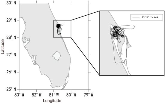
Figure 1.
RF12 flight track during SCMS95.
In the case of RF12, the small cumulus clouds form in the afternoon. These small cumulus clouds appear in the southeast of the area and move to the northwest. These clouds pass through the bay and the peninsula, then eventually move to the mainland. There is no effective surface precipitation. The temperature in clouds is always higher than 0 °C. Generally speaking, these clouds can be considered as warm-phase and non-precipitation clouds.
2.2. Model Setup: WRF-LES and SBM Scheme
Due to the small cross-sectional area of shallow convective clouds, a high-resolution numerical model is necessary to simulate the detailed structure of shallow convective clouds. For a grid resolution of 500 m, the common shallow convection covers only one or only a few grid points [37]. Therefore, large eddy simulation has become one of the best ways to simulate shallow convection [38,39]. Compared with other large-scale systems, the life cycle and scale of shallow convective clouds are shorter. Therefore, for a fixed simulation area, the entire shallow convective life cycle from formation to dissipation can be included, and detailed simulations can be obtained with large eddy simulations [40,41,42].
The Weather Research and Forecasting Model (WRF, version 3.9.1) with the built-in large eddy simulation (LES, [43]) module is used here. LES can finely analyze the energy transportation of the turbulent motion processes, and it has been widely used for turbulence research and physical process research. For the cloud microphysics scheme, single-moment or double-moment bulk parameterization schemes can capture the main features of cloud droplet size distributions, but with many assumptions [44,45,46]. The bin microphysics scheme is a better choice [47], which has been successfully applied to simulate the radiation characteristics of warm clouds and precipitation and has played a good role in simulating ice-phase clouds [48,49,50]. The fast version of spectral bin microphysics parameterization scheme (Fast-SBM, [51,52]) is used. Full-SBM has the species of cloud, rain, ice(columns), ice(plates), ice(dendrites), snow, graupel, and hail. Compared with Full-SBM, Fast-SBM combines ice(columns), ice(plates) and ice(dendrites) to ice and combines graupel and hail to graupel ([53]). Because we focus on liquid-phase clouds, the difference between Full-SBM and Fast-SBM is expected to have little effect on the results in this study. Previous studies also found that the results of Fast-SBM were similar to those of Full-SBM ([51]). For cloud droplets, spectral bin microphysics (SBM) includes 33 bins with the mass of one bin being twice the previous one. For the cloud droplet bins, the mass of the initial bin is 3.35 × 10⁻¹⁴ kg.
A 5-level nested grid area (D01, D02, D03, D04, D05, Figure 2a) is used in the simulations. LES is active on D04 and D05, which means that the boundary conditions from the real situation can be passed to D05 through D01–D04. The grid resolutions of D01–D03 are 12.5 km × 12.5 km, 2.5 km × 2.5 km and 0.5 km × 0.5 km, respectively. For the regions where large eddy simulation is active, the resolutions are D04 ~ Δx = Δy = 100 m and D05 ~ Δx = Δy = 33.3 m. Corresponding to the high horizontal resolution of 33.3 m, we are able to set a high vertical resolution. There are a total of 122 vertical levels, and the layers are dense below 5 km where the shallow convection exists. With the high resolution, the model can capture the microphysical, dynamical and thermodynamic processes well in shallow cumulus clouds. Similar resolutions have been used in previous studies [54,55]. For D04 and D05, the areas of the domains are 25.6 km × 25.6 km and 8.5 km × 8.5 km, respectively. The cumulus convection parameterization scheme is only enabled in D01. The boundary layer parameterization scheme is turned off in D04 and D05, because it is the replacement of large eddy simulation. The large-scale forcing data come from the Climate Forecast System Reanalysis (CFSR) provided by the National Centers for Environmental Prediction (NCEP), with a resolution of 0.5° × 0.5°. Lateral boundary conditions are updated every 6 h. The simulation time is from 1700 (UTC) to 2300 (UTC) and the first 3 h are taken as the spin-up time. We use the data from 2000 (UTC) to 2300 (UTC) for analysis. The model outputs the results every 15 s. As shown later in Figure 3, liquid water potential temperature, water vapor mixing ratio and cloud water mixing ratio from the simulation are consistent with observations. Therefore, we believe that it is enough to discard the first 3 h as spin-up time. At the beginning of the simulation, the relative humidity at the low level in the simulation domain (D05) is high, the surface temperature is about 29 °C and the lifting condensation level (LCL) is about 922 hPa (Figure 2b). The lower atmosphere is dominated by the southeast wind, which turns into the northeast wind above 500 hPa. Below 700 hPa, the atmosphere is humid. The cloud condensation nuclei (CCN) concentration is calculated by , where A = 500 cm−3, B = 0.5 and S is supersaturation. At the beginning of the simulation, the domain D05’s average sensible heat flux is 117.96 W·m−2 and the average latent heat flux is 180.02 W·m−2.
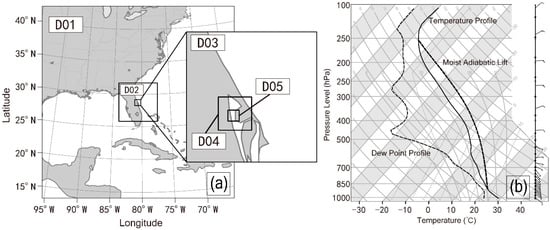
Figure 2.
(a) The five simulation domains (D01–D05). (b) The average profiles of temperature, dew point and wind at the beginning of simulation in the domain of D05.
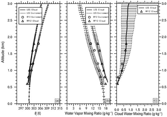
Figure 3.
Vertical profiles of properties in cloud and environment. “RF12” refers to the aircraft observation on 5 August 1995. “LES” refers to the large eddy simulation from 2000 (UTC) to 2300 (UTC) on 5 August 1995. (a) Liquid water potential temperature; (b) water vapor mixing ratio; (c) cloud water mixing ratio.
3. Methods
3.1. Methods for Calculating Cloud Physical and Microphysical Properties
As mentioned above, the shallow convective clouds in this case are all warm-phase, and cloud droplets can be assumed to be spherical particles. The mass bins obtained by the SBM can be converted into radius bins, and the radius () of the k-th mass bin is:
where is the density of liquid water and the initial value of k is 1. Because the mass of one bin is twice the previous one, Equation (1) indicates that the radius increases at the rate of, and can be expressed as:
The bin width () corresponding to the center radius of each bins is:
The number density of each bin is:
where is dry air density under standard atmospheric conditions, is the cloud water mixing ratio per unit mass of air in the k-th mass bin.
Total number concentration (N), average radius (), standard deviation of cloud droplet size distribution () and the relative dispersion of cloud droplet size distribution () can be obtained by the following equations:
respectively. Buoyancy (), virtual temperature (), cloud liquid water potential temperature (, [56]) and latent heat () are calculated by the following formulas:
Among them, the subscripts c and e represent cloud and environment, respectively; is the liquid water mixing ratio, equal to cloud water mixing ratio here, since there is no precipitation; is the water vapor mixing ratio; is the dry air specific heat capacity at constant pressure; is the mass variation at grid points only affected by condensation or evaporation within the time step and is the specific latent heat coefficient.
Cloud adiabatic fraction is obtained by the following method:
where is the adiabatic cloud water mixing ratio in the cloud.
3.2. Method for Normalizing Variables
The following method is used to normalize the physical variable x:
where is the data needing to be normalized, is the mean value of the data, s is the standard deviation of the data and the normalized data is . The normalization can transform variables to non-dimensional variables, and can be used to fairly compare two different variables.
4. Results and Discussions
4.1. Comparison of Simulations and Observations
Before comparing simulations with observations, clouds need to be selected. Consider the grids with > 0.01 g/kg as cloud and those with < 0.01 g/kg as environment. Figure 3 shows the comparison of liquid water potential temperature, water vapor mixing ratio and cloud water mixing ratio in the simulation and observation. The observational data are from the plots in Neggers et al. [36]. The liquid water potential temperature is a conserved variable in the reversible moist adiabatic motion [57], which is very convenient to analyze the wet process of the air mass during the lifting and condensation process. Whether in the cloud or in the environment, the results of the liquid water potential temperature simulated by the LES are very close to the results observed by aircraft. The simulation and observation of the water vapor mixing ratio and cloud water mixing ratio are also in good agreement. Therefore, the LES results are thought to be reliable.
Figure 4 shows cloud fraction at different heights from the simulation. The cloud fraction reaches its maximum value at 1.0 km, and then gradually decreases as the height increases. Most clouds have their cloud tops below 3.8 km. Since the lowest cloud base is around 0.6 km, the average thickness of most clouds does not exceed 3.2 km. There are also some clouds with their tops reaching 6 km or even higher. These clouds only occupy a small part and they are not analyzed here, to focus on shallow cumulus clouds. Based on aircraft observations, it is hard to determine if there were deep clouds in the field campaign, because aircraft observations only flew along a line and could not provide the whole picture of the clouds simulated here. In the simulated domain, clouds in different locations may have different cloud base heights. If the lowest cloud base height is taken to be the cloud base height for the whole domain, there would be big biases to plot vertical profiles of properties in cloud (method 1). Instead, identifying the cloud base for each cloud would cause huge computational cost (method 2). Therefore, a method different from the previous two methods is chosen. D05 is divided into 81 (9 × 9) sub-areas with each sub-area of approximately 950 m × 950 m, equivalent to the shallow cumulus cloud size. A cloud base is determined for each sub-area, where the lowest cloud grid has a cloud water mixing ratio exceeding 0.01 g/kg. In the following analysis, sub-areas of 950 m × 950 m are selected with the criteria of cloud top heights being below 3.8 km, cloud thicknesses smaller than 3.2 km and cloud base heights lower than 1.0 km. Cloud thickness is the difference between cloud top and base heights with cloud water mixing ratio greater than 0.01 g/kg.
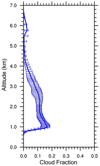
Figure 4.
The vertical profile of cloud fraction in the simulation from 2000 (UTC) to 2300 (UTC) on 5 August 1995. The cloud fraction is defined as the ratio of the number of cloud grid points to the total number of grid points. The error bars represent the data distribution range of 20–80% at the same height.
4.2. Cloud Physics Properties
Vertical profiles of properties above cloud base are needed in the following analysis. As mentioned above, D05 is divided into 81 sub-areas with each sub-area of approximately 950 m × 950 m. Vertical profiles of properties above cloud base are calculated by combining the properties in each sub-area with respect to its own cloud base.
Vertical velocity (), and in the cloud are three important cloud physics properties affecting cloud development (Figure 5). The positive vertical velocity within the cloud gradually increases from the cloud bases and reaches the maximum value near 1.0 km above the cloud bases; then the positive vertical velocity remains stable and decreases slightly with the increasing height. Instead, the absolute value of negative vertical velocity gradually increases. The mean vertical velocity changes from positive to negative near 1.8 km. The buoyancy has a similar trend with the vertical velocity, but the height at which the mean buoyancy changes from positive to negative is ~1.4 km, lower than 1.8 km for the vertical velocity, which is consistent with Newton’s law of motion. From the point of view of latent heat, the mean latent heat in the cloud is positive within about 1.0 km above the cloud bases, indicating that the lower layers are dominated by condensation. Above about 1.0 km, the mean latent heat is negative, which could be due to evaporation during entrainment.
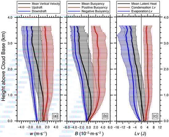
Figure 5.
Vertical profiles of (a) vertical velocity (w), (b) buoyancy (B) and (c) latent heat (Lv) from 2000 (UTC) to 2300 (UTC) on 5 August 1995. The error bars represent the data distribution range of 20–80% at the same height.
The profiles of vertical velocity, buoyancy and latent heat can explain why most clouds maintain shallow convection: the buoyancy within the cloud is suppressed and the vertical velocity is weak. The formation of shallow convection can also be explained by the large-scale forcing. The clouds form in the west of the subtropical anticyclone. Figure 6 and Figure 7 are both basic information of cloud properties. We would like to present them before introducing mechanisms in the following subsections. Figure 6 shows the cloud water mixing ratio and the cloud adiabatic fraction. The cloud water mixing ratio increases significantly from the cloud base to 1.0 km, and then increases gradually above 1.0 km; the maximum cloud water mixing ratio is achieved at ~3.2 km. The cloud base has the highest adiabatic fraction. As the height increases, the adiabatic fraction gradually decreases. Below 1.4 km, the rate of adiabatic fraction decline is the fastest; above 1.4 km, the adiabatic fraction decreases slowly and stabilizes at around 0.2. Corresponding to cloud water mixing ratio and cloud adiabatic fraction, the vertical profiles of cloud droplet spectral properties are also analyzed (Figure 7), including relative dispersion, standard deviation, number concentration and mean radius. gradually decreases with the increasing height within 0.2 km above the cloud base, and reaches the minimum mean value (~0.3) at 0.2 km. further increases until 1.0 km and then is almost constant. increases steadily with height, and the minimum is at the cloud base (1.14 μm). fluctuates slightly near the cloud base, and the maximum occurs at 0.1 km above the cloud base (206.1 cm−3). N then gradually decreases as the height increases. is similar to, and the minimum is at the cloud base (3.21 μm).
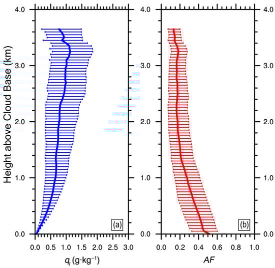
Figure 6.
Vertical profiles of (a) cloud water mixing ratio (), and (b) cloud adiabatic fraction () in the simulation from 2000 (UTC) to 2300 (UTC) on 5 August 1995. The error bars represent the data distribution range of 20–80% at the same height.
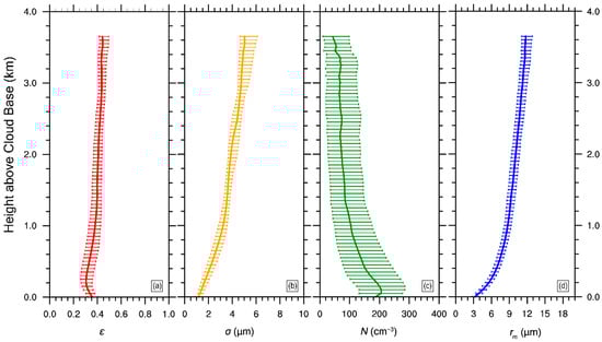
Figure 7.
Vertical profiles of cloud droplet spectral properties: (a) relative dispersion, (b) standard deviation (), (c) number concentration (), (d) mean radius in the simulation from 2000 (UTC) to 2300 (UTC) on 5 August 1995. The error bars represent the data distribution range of 20–80% at the same height.
4.3. Effects of Standard Deviation and Mean Radius on Relative Dispersion
Since is the ratio of to , it is critical to analyze the variations of and . Figure 7 shows that, the variation of with height is not monotonic, different from the variations of and that increase with the increasing height. Since and are both dimensional variables, they need to be transformed into non-dimensional variables with the normalized method in Section 3.2 (Figure 8a,b). The variability of the two variables within each 50 m height is analyzed (Figure 8c,d). If we take the derivative of Equation (8) by height (), we have
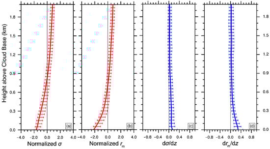
Figure 8.
Vertical profiles of (a) normalized standard deviation , (b) normalized mean radius , (c) variation rate of normalized standard deviation with height (), (d) variation rate of normalized mean radius with height (). The error bars represent the data distribution range of 20–80% at the same height. The simulation is from 2000 (UTC) to 2300 (UTC) on 5 August 1995.
From Equation (15), the sign of is determined by a cross multiplication difference:
In Equation (16), the influencing factors of the variation of relative dispersion with height can be divided into two categories, namely, the change rate of the variable with height () and the value of the variable at a certain height. Since each term is of the same form, it is possible to estimate the positive or negative difference of the multiplication by simply subtracting the factors of the multiplication. Figure 9 is the normalized vertical profiles of and . However, it should be noted that as the height increases, the values of and become larger, and the above method may not work well. Therefore, only the data with the largest changes below 2.0 km are analyzed. It can be seen from Figure 9 that from the cloud base to 0.2 km, both and are mainly negative, which together determines the decreasing trend of relative dispersion with the increasing height (Figure 7a). In the range of 0.2–1 km, the increasing trend of relative dispersion with height mainly comes from positive . In the range of 1–2 km, both and are near 0, so the relative dispersion changes slowly with height.
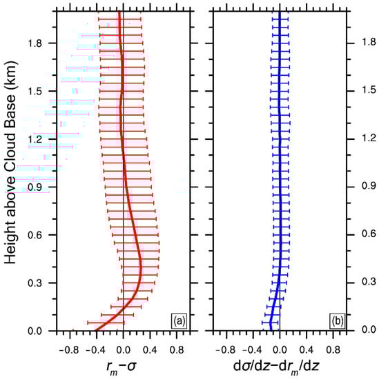
Figure 9.
Vertical profiles of (a) the difference between the normalized mean radius () and the normalized standard deviation (), (b) the vertical variability of the normalized standard deviation () minus the vertical variability of the normalized mean radius (). The error bars represent the data distribution range of 20–80% at the same height. The simulation is from 2000 (UTC) to 2300 (UTC) on 5 August 1995.
Besides , it is very important to analyze cloud droplet size distributions, since represents the width of cloud droplet size distribution. Figure 10 illustrates that, cloud droplets of 2–5 μm gradually decrease with the increasing height below 0.2 km, and cloud droplets of 5–10 μm begin to appear and increase rapidly. This is in line with the characteristics of the cloud base itself. In the cloud base, a large number of cloud condensation nuclei are activated into small cloud droplets, and the condensation rate is large for the small droplets according to the adiabatic condensation theory [58]; as a result, the small droplets grow rapidly. This explains why the within 0.2 km is large (Figure 8d). Because of the fast increase in , decreases with the increasing height. The increase in above 0.2 km is related to entrainment-mixing processes. The radius of a large number of cloud droplets are in the range of 10–15 μm, but collision-coalescence is still thought to be weak. However, because of the entrainment of dry air either through the lateral boundary, cloud top or both, some droplets evaporate into small droplets, which leads to the increase of. One evidence is that cloud droplets less than 10 μm always exist, and do not significantly reduce with height.
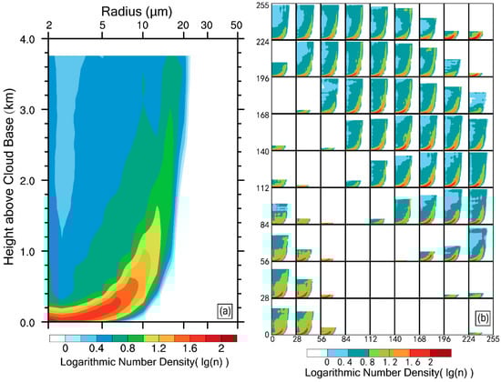
Figure 10.
Vertical variations of cloud droplet size distributions (a) in the whole domain and (b) in each sub-area, with the numbers on the X-axis and Y-axis indicating the grids in domain D05.
4.4. Effects of Vertical Velocity and Entrainment on Relative Dispersion
In addition to and , which can directly affect, and in the cloud can affect through physical processes [20,22,58]. Figure 11 shows a negative correlation between the relative dispersion and vertical velocity, and the correlation coefficient is −0.54. The negative correlation is consistent with previous studies [59,60]. On the one hand, larger w increases supersaturation, and further enhances condensational growth [61]. Larger supersaturation corresponds to narrower cloud droplet size distributions, in other words, smaller [17]. On the other hand, for larger w, less dry air is entrained into cloud [58,62,63] and droplet evaporation is weaker. As a result, broadening of cloud droplet size distribution during entrainment-mixing is weakened, in other words, smaller . Oppositely, when w is smaller or even negative, entrainment becomes stronger. Some droplets could evaporate faster than others and cloud droplet size distributions broaden significantly, in other words, larger [64].
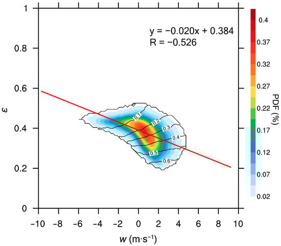
Figure 11.
Relationship between dispersion () and vertical velocity () at all heights. The black contour is adiabatic fraction (). The simulation is from 2000 (UTC) to 2300 (UTC) on 5 August 1995.
Figure 11 further shows that more than 3 × 10⁵ data points form a single-centered distribution with the center concentrated in of 0.3–0.4 and w of 0–2 m/s. According to the vertical profiles of relative dispersion (Figure 7a), vertical velocity (Figure 5a) and cloud fraction (Figure 4), most of these center points come from 0 to 2.0 km near the cloud base. The data points with large relative dispersion (0.4–0.5) and downdraft (w ~ −3 to 0 m/s) are mainly from the cloud upper part or the cloud top. Therefore, it is necessary to separately discuss the relationship between and w at different heights from the cloud base. In addition, with the increase of w, increases and decreases, which means that the cloud tends to be more adiabatic and cloud droplet size distribution tends to be narrower. When w is smaller, is also smaller and is larger. Therefore, evaporation during entrainment broadens cloud droplet size distributions.
The relationship between and is fitted every 50 m. Figure 12a shows part of the relationships for every 400 m. Figure 12b,c shows the correlation coefficient and the slope of the linear regression equation as a function of height. Near the cloud base, the correlation coefficient is around −0.45 and the slope is around −0.02. As the height increases, the correlation coefficient and slope are both negative and their absolute values increase to the maximum absolute values of −0.59 and −0.04, respectively. As the height further increases, the number of data points decreases, and the center of the data points also moves from the area with positive w and small to the area with negative w and big , which is consistent with Figure 11. The physical mechanisms are summarized below. Near the cloud base, on the one hand, larger vertical velocity (updraft) makes cloud droplet activation more active, and more small droplets are formed to increase relative dispersion; on the other hand, larger vertical velocity increases supersaturation, promotes condensation and reduces relative dispersion. The two factors contradict each other and the negative relationship between and w is weak near the cloud base [65,66]. The latter factor is expected to dominate over the former one with the increasing height, because activation becomes weaker at higher heights. Therefore, the degree of negative correlation between and w increases to its maximum with the increasing height. As the height continues to increase, the cloud droplet size distributions tend to stabilize (Figure 10), and the relative dispersion range decreases. As a result, both of absolute values of the correlation coefficient and the slope between relative dispersion and vertical velocity decrease.
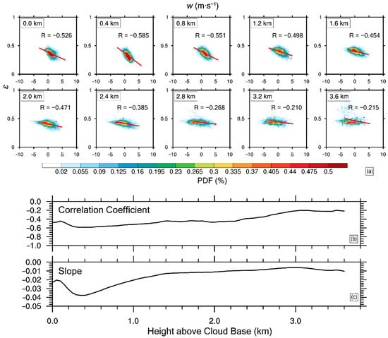
Figure 12.
(a) Relationships between relative dispersion () and vertical velocity () at typical heights; the variations of (b) correlation coefficients and (c) slopes of at every 50 m with height. The simulation from 2000 (UTC) to 2300 (UTC) on 5 August 1995.
The above analysis indicates that the adiabatic fraction of the cloud is also an important factor affecting the relative dispersion of cloud droplet size distribution [17,19]. Similar to Figure 11, Figure 13 shows a negative correlation between and with the correlation coefficient of −0.79. Larger means that the cloud is less affected by entrainment of dry air, which results in weaker evaporation and smaller . Similar to Figure 12, Figure 14 shows the relationship between and for different heights. and have the weakest correlation near the cloud base, with the correlation coefficient of −0.22. Since has the largest value near the cloud base, it is expected to have small . However, as mentioned above, the strong activation of droplets near the cloud base increases, which contradicts the effect of . Therefore, the relationship between and is weak. As the height increases, the activation intensity decreases, and the influence of entrainment on increases; as a result, the absolute value of the negative correlation coefficient increases rapidly, with the maximum of −0.84. As the height continues to increase, the cloud droplet size distribution tends to stabilize (Figure 10), and the relative dispersion range decreases; therefore, the correlation coefficient between and decreases. The variation of slope is generally similar to that of the correlation coefficient. In the upper part of the cloud, the absolute value of slope increases, which could be due to the small range (<0.4). Since is the ratio of to , Figures S1 and S3 in the Supplementary Materials show the relationship of , with for all heights, respectively. Figures S2 and S4 are for different heights. Generally, the relationship of with is similar to that of . As expected, is positively correlated with at each height (Figure S4). For a larger , entrainment and evaporation are weaker, so is larger. With the increasing height, the slope of the relationship between and increases, which contributes to the increasing absolute slope (negative) of the relationship between and (Figure 14). Interestingly, when the data at all heights are combined, and are negatively correlated. As shown in Figure S2, the black ellipses schematically show the positive relationships between and at different heights. So, the negative relationship between and at all heights is caused by the varying height, in other words, the combination of the negative relationships between and at different heights. Figure 15 is plotted to show the vertical variations of , and considering different . It is clear that for the same height, decreases, decreases and increases for the increasing . This is consistent with theoretical expectation that for a more diluted cloud (smaller ), cloud droplet size distributions are wider (larger and ) and droplet sizes are smaller (smaller ). Figure 16 shows direct relationships of , and with cloud drop number concentration. All of , and are negatively correlated with number concentration. When is larger, a cloud is less affected by entrainment and number concentration is larger. As explained above, and are expected to be smaller in more adiabatic clouds. Prabha et al. [28] found that the relationships of , and with cloud drop number concentration were different under premonsoon and monsoon clouds. The negative relationship between and number concentration is consistent with many previous studies [59,67,68], but different from others [23,30].
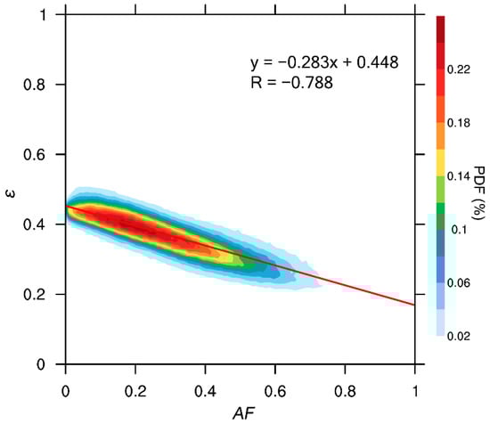
Figure 13.
Relationship between relative dispersion () and cloud adiabatic fraction () at all heights. The simulation is from 2000 (UTC) to 2300 (UTC) on 5 August 1995.
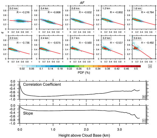
Figure 14.
(a) Relationships between relative dispersion () and cloud adiabatic fraction () at typical heights, the variations of (b) correlation coefficients and (c) slopes of at every 50 m with height. The simulation is from 2000 (UTC) to 2300 (UTC) on 5 August 1995.
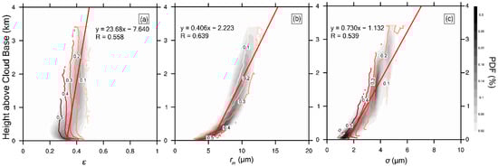
Figure 15.
Distributions of (a) relative dispersion, (b) mean radius and (c) standard deviation with height. The black contour is adiabatic fraction. The simulation is from 2000 (UTC) to 2300 (UTC) on 5 August 1995.
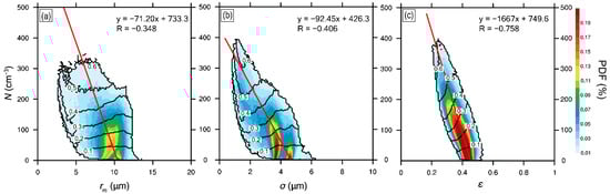
Figure 16.
Relationships between number concentration and (a) mean radius (), (b) standard deviation () and (c) relative dispersion (). The black contour is adiabatic fraction (). The simulation is from 2000 (UTC) to 2300 (UTC) on 5 August 1995.
, and are negatively correlated with small droplet number concentration (radius ≤10 μm, Figure 17a–c), respectively, similar to the relationships of , and with the total droplet number concentration (Figure 16). and have weak negative correlations with large droplet number concentration (radius >10 μm, Figure 17d,e) and has a weak positive correlation with large droplet number concentration. For larger , both small and large droplet number concentrations are larger due to weaker entrainment and dilution. Prabha et al. [28] analyzed the relationships of , and with small droplet number concentration and . They found that the small droplet number concentration decreased when increased; for a given , decreased when the small droplet number concentration increased; was larger in the more adiabatic clouds; was negatively correlated with the small droplet number concentration in two premonsoon cases and one monsoon case.
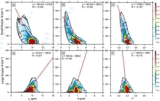
Figure 17.
Relationships between small (radius ≤10 μm) and large (radius >10 μm) droplet number concentrations and (a,d) mean radius (), (b,e) standard deviation (), (c,f) relative dispersion (), respectively. The black contour is . The simulation is from 2000 (UTC) to 2300 (UTC) on 5 August 1995.
In addition to using, the cloud droplet size distributions at different distances from the cloud core can also be analyzed to explore the impact of entrainment; at different heights, divide into different ranges and plot the cloud droplet size distribution in 4 typical ranges at the 1 km height, as shown in Figure 18. At the same height, from the edge to the core with increasing , decreases, increases slightly, and the peak of the cloud droplet size distribution gradually moves towards the big droplets. The reason is that the degree of adiabaticity increases from the boundary to the core, and the effect of evaporation due to entrainment is weakened.
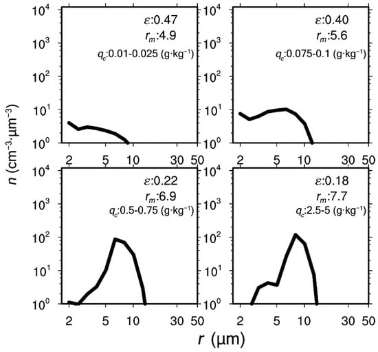
Figure 18.
Cloud droplet size distributions in different cloud water mixing ratio () at the 1 km height. is relative dispersion and is mean radius. The simulation is from 2000 (UTC) to 2300 (UTC) on 5 August 1995.
5. Summary
To analyze the factors affecting relative dispersion of cloud droplet size distributions, shallow convective clouds are simulated by large eddy simulation. The simulation results are first verified by aircraft observations by comparing vertical profiles of liquid water potential temperature and water vapor mixing ratio in cloud and environment. After that, vertical profiles of vertical velocity, buoyancy, latent heat, cloud water mixing ratio and cloud adiabatic fraction are plotted to understand the general macro characteristics of the simulated shallow cumulus clouds.
Since relative dispersion is the ratio of standard deviation to mean radius, it is naturally important to analyze the effects of standard deviation and mean radius on relative dispersion. From the cloud base to 0.2 km, relative dispersion decreases with the increasing height, which is mainly due to negative and . The increase in relative dispersion with the increasing height in the range of 0.2–1 km is mainly due to positive . Relative dispersion changes slowly with height above 1 km.
Besides standard deviation and mean radius, relative dispersion is significantly affected by vertical velocity in cloud and entrainment-mixing processes. Both of the relationships between relative dispersion and vertical velocity, and between relative dispersion and adiabatic fraction are negative. Larger positive vertical velocity increases supersaturation and corresponds to narrower cloud droplet size distributions. Larger adiabatic fraction means that the cloud is less affected by evaporation during entrainment of dry air, in other words, narrower cloud droplet size distributions. The impact of entrainment is also examined by analyzing cloud droplet size distributions at different distances from the cloud core. When entrainment weakens from the edge to the core, relative dispersion decreases.
It is interesting to note that the negative relationships are relatively weak near the cloud base, become the strongest in the middle of clouds, and then weaken with further increasing height. The weak relationship between relative dispersion and vertical velocity near the cloud base is due to the two contradicting factors: larger vertical velocity causes more active droplet activation to increase relative dispersion; as mentioned above, larger vertical velocity also reduces relative dispersion by increasing supersaturation. With the increasing height, the latter factor dominates the former one to produce the strongest relationship between relative dispersion and vertical velocity. The relationship weakens with further increasing height because the relative dispersion range decreases. Similarly, the weak relationship between relative dispersion and adiabatic fraction near the cloud base is related to the strong activation of droplets. With increasing height, the influence of entrainment dominates the activation intensity, thus the negative relationship strengthens. The relative dispersion range decreases with further increasing height, so the negative relationship weakens.
It is confirmed that when vertical velocity and entrainment dominate, relative dispersion is negatively correlated with number concentration. The mechanisms are that supersaturation is larger for larger vertical velocity, which further causes stronger activation (larger number concentration) and stronger condensational growth (smaller relative dispersion) [59,60]; for smaller adiabatic fractions, entrainment is stronger, which decreases number concentration and increases relative dispersion [69,70]. However, this study does not consider the effects of aerosol, which may cause a positive correlation between relative dispersion and number concentration [23]. In future studies, the effects of aerosol on relative dispersion, vertical velocity and adiabatic fraction will be included and the relationship between relative dispersion and number concentration will be analyzed more comprehensively.
Supplementary Materials
The following are available online at https://www.mdpi.com/article/10.3390/atmos12040485/s1, Figure S1: The relationship between standard deviation (σ) and cloud adiabatic fraction () at all heights, Figure S2: (a) Relationships between standard deviation (σ) and adiabatic fraction (AF) at typical heights; the varia-tions of (b) correlation coefficients and (c) slopes of σ vs AF at every 50 m with height, Figure S3: The relationship between mean radius (rm) and cloud adiabatic fraction (AF) at all heights. The ellipses schematically show the positive relationships between rm and AF at different heights, Figure S4: (a) Relationships between mean radius (rm) and adiabatic fraction (AF) at typical heights; the variations of (b) correlation coefficients and (c) slopes of rm vs AF at every 50 m with height.
Author Contributions
Conceptualization, Z.Z. and C.L.; formal analysis, Z.Z., C.L., X.J. and F.Y.; software, Z.Z.; writing—original draft, Z.Z.; writing—review and editing, C.Y., C.L., X.J., F.Y., Y.Q. and M.C. All authors have read and agreed to the published version of the manuscript.
Funding
This research was funded by the National Key Research and Development Program of China, grant number: 2019YFA0606803, the Second Tibetan Plateau Scientific Expedition and Research (STEP) program, grant number: 2019QZKK0105, the National Natural Science Foundation of China, grant number: 42027804, 42075073 and 41975181, the Qinglan Project, grant number: R2018Q05.
Institutional Review Board Statement
Not applicable.
Informed Consent Statement
Not applicable.
Data Availability Statement
Data set available on request to corresponding authors.
Acknowledgments
The observational results are from the plots in Neggers et al. ([36]). This research is supported by the National Key Research and Development Program of China (2019YFA0606803), the Second Tibetan Plateau Scientific Expedition and Research (STEP) program (2019QZKK0105), the National Natural Science Foundation of China (42027804, 42075073, 41975181), the Qinglan Project (R2018Q05), and the National Center of Meteorology, Abu Dhabi, UAE, under the UAE Research Program for Rain Enhancement Science.
Conflicts of Interest
The authors declare no conflict of interest.
References
- Takemi, T.; Hirayama, O.; Liu, C. Factors responsible for the vertical development of tropical oceanic cumulus convection. Geophys. Res. Lett. 2004, 31, 167–174. [Google Scholar] [CrossRef]
- Yanai, M.; Johnson, R.H. Impacts of cumulus convection on thermodynamic fields. In The Representation of Cumulus Convection in Numerical Models; Springer: New York, NY, USA, 1993; pp. 39–62. [Google Scholar]
- Li, Y.; Zhang, M. The role of shallow convection over the Tibetan plateau. J. Clim. 2017, 30, 5791–5803. [Google Scholar] [CrossRef]
- Nuijens, L.; Stevens, B.; Siebesma, A.P. The environment of precipitating shallow cumulus convection. J. Atmos. Sci. 2009, 66, 1962–1979. [Google Scholar] [CrossRef]
- Jiang, X.; Liu, Q.; Ma, Z. Influences of shallow convective process and boundary-layer clouds on cloud forecast in GRAPES Global Model. Meteorol. Mon. 2015, 41, 921–931. [Google Scholar]
- Zhang, F.; Wu, K.; Li, J.; Zhang, H.; Hu, S. Radiative transfer in the region with solar and infrared spectra overlap. J. Quant. Spectrosc. Radiat. Transf. 2018, 219, 366–378. [Google Scholar] [CrossRef]
- Betts, A.K. A new convective adjustment scheme. Part. I: Observational and theoretical basis. Q. J. R. Meteorol. Soc. 1986, 112, 677–691. [Google Scholar]
- Tiedtke, M.; Heckley, W.; Slingo, J. Tropical forecasting at ECMWF: The influence of physical parametrization on the mean structure of forecasts and analyses. Q. J. R. Meteorol. Soc. 1988, 114, 639–664. [Google Scholar] [CrossRef]
- Lord, S.J.; Chao, W.C.; Arakawa, A. Interaction of a cumulus cloud ensemble with the large-scale environment. Part. IV: The discrete model. J. Atmos. Sci. 1982, 39, 104–113. [Google Scholar] [CrossRef]
- Sakradzija, M.; Seifert, A.; Dipankar, A. A stochastic scale-aware parameterization of shallow cumulus convection across the convective gray zone. J. Adv. Model. Earth Syst. 2016, 8, 786–812. [Google Scholar] [CrossRef]
- Pergaud, J.; Masson, V.; Malardel, S.; Couvreux, F. A parameterization of dry thermals and shallow cumuli for mesoscale numerical weather prediction. Bound. Layer Meteorol. 2009, 132, 83. [Google Scholar] [CrossRef]
- Luo, S.; Lu, C.; Guo, X.; Li, Y.; Xue, S. Numerical simulation of the effects of entrainment-mixing on cloud droplet size distributions and microphysical properties over the Tibetan Plateau. China Sci. Pap. 2017, 12, 972–977. [Google Scholar]
- Lei, H.; Hong, Y.; Zhao, Z.; Xiao, H.; Guo, X. Advances in cloud and precipitation physics and weather modification in recent years. Chin. J. Atmos. Sci. 2008, 32, 967–974. [Google Scholar]
- Haynes, J.M.; Stephens, G.L. Tropical oceanic cloudiness and the incidence of precipitation: Early results from CloudSat. Geophys. Res. Lett. 2007, 34, 1–5. [Google Scholar] [CrossRef]
- Liu, Y.; Lu, C.; Li, W. Skewness of cloud droplet spectrum and an improved estimation for its relative dispersion. Meteorol. Atmos. Phys. 2017, 129, 47–56. [Google Scholar] [CrossRef]
- Zhou, G.; Zhao, C.; Qin, Y. Impact of cloud droplets spectral uncertainty on mesoscale precipitation. J. Trop. Meteorol. 2005, 21, 605–614. [Google Scholar]
- Yum, S.S.; Hudson, J.G. Adiabatic predictions and observations of cloud droplet spectral broadness. Atmos. Res. 2005, 73, 203–223. [Google Scholar] [CrossRef]
- Zhao, C.; Tie, X.; Brasseur, G.; Noone, K.J.; Nakajima, T.; Zhang, Q.; Zhang, R.; Huang, M.; Duan, Y.; Li, G.; et al. Aircraft measurements of cloud droplet spectral dispersion and implications for indirect aerosol radiative forcing. Geophys. Res. Lett. 2006, 33, 1–4. [Google Scholar] [CrossRef]
- Pawlowska, H.; Grabowski, W.W.; Brenguier, J.L. Observations of the width of cloud droplet spectra in stratocumulus. Geophys. Res. Lett. 2006, 33, 1–5. [Google Scholar] [CrossRef]
- Zhao, C.; Zhao, L.; Dong, X. A case study of stratus cloud properties using in situ aircraft observations over Huanghua, China. Atmosphere 2019, 10, 19. [Google Scholar] [CrossRef]
- Lu, C.; Liu, Y.; Yum, S.S.; Chen, J.; Zhu, L.; Gao, S.; Yin, Y.; Jia, X.; Wang, Y. Reconciling contrasting relationships between relative dispersion and volume-mean radius of cloud droplet size distributions. J. Geophys. Res. Atmos. 2020, 125, e2019JD031868. [Google Scholar] [CrossRef]
- Zhu, L.; Lu, C.; Gao, S.; Soo, Y.S. Spectral width of cloud droplet spectra and its impact factors in marine stratocumulus. Chin. J. Atmos. Sci. 2020, 44, 575–590. [Google Scholar]
- Liu, Y.; Daum, P.H. Anthropogenic aerosols: Indirect warming effect from dispersion forcing. Nature 2002, 419, 580. [Google Scholar] [CrossRef]
- Liu, Y.; Daum, P.H.; McGraw, R.L. Size truncation effect, threshold behavior, and a new type of autoconversion parameterization. Geophys. Res. Lett. 2005, 32, 1–5. [Google Scholar] [CrossRef]
- Xie, X.; Zhang, H.; Liu, X.; Peng, Y.; Liu, Y. Sensitivity study of cloud parameterizations with relative dispersion in CAM5. 1: Impacts on aerosol indirect effects. Atmos. Chem. Phys. 2017, 17, 5877–5892. [Google Scholar] [CrossRef]
- Xie, X.I.; Liu, X.I.; Peng, Y.; Wang, Y.I.; Yue, Z.; Li, X.I. Numerical simulation of clouds and precipitation depending on different relationships between aerosol and cloud droplet spectral dispersion. Tellus B Chem. Phys. Meteorol. 2013, 65, 19054. [Google Scholar] [CrossRef]
- Lu, C.S.; Liu, Y.G.; Niu, S.J.; Xue, Y. Broadening of cloud droplet size distributions and warm rain initiation associated with turbulence: An overview. Atmos. Ocean. Sci. Lett. 2018, 11, 123–135. [Google Scholar] [CrossRef]
- Thara, P.; Patade, S.; Pandithurai, G.; Khain, A.; Axisa, D.; Kumar, P.; Maheshkumar, R.S.; Kulkarni, J.R.; Goswami, B.N. Spectral width of premonsoon and monsoon clouds over Indo-Gangetic valley. J. Geophys. Res. 2012, 117, D20205. [Google Scholar]
- Anil Kumar, V.; Pandithurai, G.; Leena, P.P. Investigation of aerosol indirect effects on monsoon clouds using ground-based measurements over a high-altitude site in Western Ghats. Atmos. Chem. Phys. 2016, 16, 8423–8430. [Google Scholar] [CrossRef]
- Pandithurai, G.; Dipu, S.; Prabha, T.V.; Maheskumar, R.S.; Kulkarni, J.R.; Goswami, B.N. Aerosol effect on droplet spectral dispersion in warm continental cumuli. J. Geophys. Res. 2012, 117, D16202. [Google Scholar] [CrossRef]
- Chandrakar, K.K.; Cantrell, W.; Chang, K.; Ciochetto, D.; Yang, F. Aerosol indirect effect from turbulence-induced broadening of cloud-droplet size distributions. Proc. Natl. Acad. Sci. USA 2016, 113, 14243. [Google Scholar] [CrossRef]
- Ma, J.; Chen, Y.; Wang, W.; Yan, P.; Liu, H. Strong air pollution causes widespread haze-clouds over China. J. Geophys. Res. Atmos. 2010, 155, D18204. [Google Scholar] [CrossRef]
- Desai, N.; Glienke, S.; Fugal, J.; Shaw, R.A. Search for microphysical signatures of stochastic condensation in marine boundary layer clouds using airborne digital holography. J. Geophys. Res. Atmos. 2019, 124, 2739–2752. [Google Scholar] [CrossRef]
- Weckwerth, T.; Horst, T.; Wilson, J. An observational study of the evolution of horizontal convective rolls. Mon. Weather Rev. 1999, 127, 2160–2179. [Google Scholar] [CrossRef]
- Rodts, S.M.A.; Peter, G.D.; Harm, J.J. Size distributions and dynamical properties of shallow cumulus clouds from aircraft observations and satellite data. J. Atmos. Sci. 2003, 60, 1895–1912. [Google Scholar] [CrossRef]
- Neggers, R.; Duynkerke, P.; Rodts, S. Shallow cumulus convection: A validation of large-eddy simulation against aircraft and Landsat observations. Q. J. R. Meteorol. Soc. J. Atmos. Sci. Appl. Meteorol. Phys. Oceanogr. 2003, 129, 2671–2696. [Google Scholar] [CrossRef]
- Brown, A.R. The sensitivity of large-eddy simulations of shallow cumulus convection to resolution and subgrid model. Q. J. R. Meteorol. Soc. 1999, 125, 469–482. [Google Scholar] [CrossRef]
- Dawe, J.T.; Austin, P.H. Statistical analysis of an LES shallow cumulus cloud ensemble using a cloud tracking algorithm. Atmos. Chem. Phys. 2012, 12, 101–1119. [Google Scholar] [CrossRef]
- Jiang, H.; Xue, H.; Teller, A.; Feingold, G.; Levin, Z. Aerosol effects on the lifetime of shallow cumulus. Geophys. Res. Lett. 2006, 33. [Google Scholar] [CrossRef]
- Zhao, M.; Austin, P.H. Life cycle of numerically simulated shallow cumulus clouds. Part. I: Transport. J. Atmos. Sci. 2005, 62, 1269–1290. [Google Scholar] [CrossRef]
- Zhao, M.; Austin, P.H. Life cycle of numerically simulated shallow cumulus clouds. Part. II: Mixing dynamics. J. Atmos. Sci. 2005, 62, 1291–1310. [Google Scholar] [CrossRef]
- Xu, X.; Xue, H. Impacts of free-tropospheric temperature and humidity on nocturnal nonprecipitating marine stratocumulus. J. Atmos. Sci. 2015, 72, 2853–2864. [Google Scholar] [CrossRef]
- Moeng, C.; Dudhia, J.; Klemp, J.; Sullivan, P. Examining two-way grid nesting for large eddy simulation of the PBL using the WRF model. Mon. Weather Rev. 2007, 135, 2295–2311. [Google Scholar] [CrossRef]
- von Salzen, K.; McFarlane, N.A. Parameterization of the bulk effects of lateral and cloud-top entrainment in transient shallow cumulus clouds. J. Atmos. Sci. 2002, 59, 1405–1430. [Google Scholar] [CrossRef]
- Bretherton, C.S.; Park, S. A new bulk shallow-cumulus model and implications for penetrative entrainment feedback on updraft buoyancy. J. Atmos. Sci. 2008, 65, 2174–2193. [Google Scholar] [CrossRef]
- Slawinska, J.; Grabowski, W.W.; Pawlowska, H.; Wyszogrodzki, A.A. Optical properties of shallow convective clouds diagnosed from a bulk-microphysics large-eddy simulation. J. Clim. 2008, 21, 1639–1647. [Google Scholar] [CrossRef]
- Seifert, A.; Khain, A.; Pokrovsky, A.; Beheng, K.D. A comparison of spectral bin and two-moment bulk mixed-phase cloud microphysics. Atmos. Res. 2006, 80, 46–66. [Google Scholar] [CrossRef]
- Suzuki, K.; Nakajima, T.; Nakajima, T.Y.; Khain, A.P. A study of microphysical mechanisms for correlation patterns between droplet radius and optical thickness of warm clouds with a spectral bin microphysics cloud model. J. Atmos. Sci. 2010, 67, 1126–1141. [Google Scholar] [CrossRef]
- Lynn, B.; Khain, A. Utilization of spectral bin microphysics and bulk parameterization schemes to simulate the cloud structure and precipitation in a mesoscale rain event. J. Geophys. Res. Atmos. 2007, 112, D22205S. [Google Scholar] [CrossRef]
- Fan, J.; Ovtchinnikov, M.; Comstock, J.M.; McFarlane, S.A.; Khain, A. Ice formation in Arctic mixed-phase clouds: Insights from a 3-D cloud-resolving model with size-resolved aerosol and cloud microphysics. J. Geophys. Res. Atmos. 2009, 114, D04205. [Google Scholar] [CrossRef]
- Khain, A.; Leung, L.; Lynn, B.; Ghan, S. Effects of aerosols on the dynamics and microphysics of squall lines simulated by spectral bin and bulk parameterization schemes. J. Geophys. Res. Atmos. 2009, 114, D22203. [Google Scholar] [CrossRef]
- Skamarock, W.C.; Klemp, J.B.; Dudhia, J.; Gill, D.O.; Barker, D.M.; Wang, W.; Powers, J.G. A description of the Advanced Research WRF version 3 [cited 2008 June]. NCAR Tech. Note 2008. [Google Scholar] [CrossRef]
- Wang, W.; Bruyère, C.; Duda, M.; Dudhia, J.; Gill, D.; Kavulich, M.; Keene, K.; Chen, M.; Lin, H.-C.; Michalakes, J.; et al. User’s Guide for the Advanced Research WRF (ARW) Modeling System Version 3.9. 2017 [cited 2017 April 17]. Available online: https://www2.mmm.ucar.edu/wrf/users/docs/user_guide_V3/user_guide_V3.9/contents.html (accessed on 11 April 2021).
- Seifert, A.; Heus, T. Large-eddy simulation of organized precipitating trade wind cumulus clouds. Atmos. Chem. Phys. 2013, 13, 5631–5645. [Google Scholar] [CrossRef]
- Matheou, G.; Chung, D.; Nuijens, L.; Stevens, B.; Teixeira, J. On the fidelity of large-eddy simulation of shallow precipitating cumulus convection. Mon. Weather Rev. 2011, 139, 2918–2939. [Google Scholar] [CrossRef]
- Sommeria, G.; Deardorff, J.W. Subgrid-Scale Condensation in Models of Nonprecipitating Clouds. J. Atmos. Sci. 1977, 34, 344–355. [Google Scholar] [CrossRef]
- Lu, C.; Sun, C.; Liu, Y.; Zhang, G.J.; Lin, Y.; Gao, W.; Niu, S.; Yin, Y.; Qiu, Y.; Jin, L. Observational relationship between entrainment rate and environmental relative humidity and implications for convection parameterization. Geophys. Res. Lett. 2018, 45, 13–495. [Google Scholar] [CrossRef]
- Lu, C.; Liu, Y.; Niu, S.; Vogelmann, A.M. Observed impacts of vertical velocity on cloud microphysics and implications for aerosol indirect effects. Geophys. Res. Lett. 2012, 39, L21808. [Google Scholar] [CrossRef]
- Berg, L.K.; Berkowitz, C.M.; Barnard, J.C.; Senum, G.; Springston, S.R. Observations of the first aerosol indirect effect in shallow cumuli. Geophys. Res. Lett. 2011, 38, L03809. [Google Scholar] [CrossRef][Green Version]
- Lu, C.; Liu, Y.; Zhang, G.J.; Wu, X.; Endo, S.; Cao, L.; Li, Y.; Guo, X. Improving parameterization of entrainment rate for shallow convection with aircraft measurements and large-eddy simulation. J. Atmos. Sci. 2016, 73, 761–773. [Google Scholar] [CrossRef]
- Yau, K.M.; Rogers, R.R. A Short Course in Cloud Physics; Pergamon Press: Oxford, UK, 1979. [Google Scholar]
- Zhang, G.J.; Wu, X.; Zeng, X.; Mitovski, T. Estimation of convective entrainment properties from a cloud-resolving model simulation during TWP-ICE. Clim. Dyn. 2016, 47, 2177–2192. [Google Scholar] [CrossRef]
- Neggers, R.A.J.; Siebesma, A.P.; Jonker, H.J.J. A multiparcel model. for shallow cumulus convection. J. Atmos. 2002, 59, 1655–1668. [Google Scholar] [CrossRef]
- Lu, C.; Niu, S.; Liu, Y.; Vogelmann, A.M. Empirical relationship between entrainment rate and microphysics in cumulus clouds. Geophys. Res. Lett. 2013, 40, 2333–2338. [Google Scholar] [CrossRef]
- Leaitch, W.; Banic, C.; Isaac, G.; Couture, M.; Liu, P.; Gultepe, I.; Li, S.M.; Kleinman, L.; Daum, P.; MacPherson, J. Physical and chemical observations in marine stratus during the 1993 North. Atlantic Regional Experiment: Factors controlling cloud droplet number concentrations. J. Geophys. Res. Atmos. 1996, 101, 29123–29135. [Google Scholar] [CrossRef]
- Brenguier, J.-L.; Pawlowska, H.; Schüller, L.; Preusker, R.; Fischer, J.; Fouquart, Y. Radiative properties of boundary layer clouds: Droplet effective radius versus number concentration. J. Atmos. Sci. 2000, 57, 803–821. [Google Scholar] [CrossRef]
- Desai, N.; Chandrakar, K.K.; Chang, K.; Cantrell, W.; Shaw, R.A. Influence of microphysical variability on stochastic condensation in a turbulent laboratory cloud. J. Atmos. Sci. 2017, 75, 189–201. [Google Scholar] [CrossRef]
- Chandrakar, K.K.; Cantrell, W.; Shaw, R.A. Influence of turbulent fluctuations on cloud droplet size dispersion and aerosol indirect effects. J. Atmos. Sci. 2018, 75, 29123–29135. [Google Scholar] [CrossRef]
- Bipin, K.; Götzfried, P.; Suresh, N.; Schumacher, J.; Shaw, R. Scale dependence of cloud microphysical response to turbulent entrainment and mixing. J. Adv. Model. Earth Syst. 2018, 10, 2777–2785. [Google Scholar] [CrossRef]
- TöLle, M.H.; Krueger, S.K. Effects of entrainment and mixing on droplet size distributions in warm cumulus clouds. J. Adv. Model. Earth Syst. 2014, 6, 281–299. [Google Scholar] [CrossRef]
Publisher’s Note: MDPI stays neutral with regard to jurisdictional claims in published maps and institutional affiliations. |
© 2021 by the authors. Licensee MDPI, Basel, Switzerland. This article is an open access article distributed under the terms and conditions of the Creative Commons Attribution (CC BY) license (https://creativecommons.org/licenses/by/4.0/).