Article

Monitoring Air Pollution Variability during Disasters

Department of Urban Planning and Environmental Policy, Texas Southern University, Houston, TX 77004, USA
Atmosphere 2021, 12(4), 420; https://doi.org/10.3390/atmos12040420
Submission received: 5 March 2021 / Revised: 21 March 2021 / Accepted: 22 March 2021 / Published: 25 March 2021
(This article belongs to the Special Issue Advances in Air Quality Data Analysis and Modeling)

Abstract

:
National environmental regulations lack short-term standards for variability in fine particulate matter (PM2.5); they depend solely on concentration-based standards. Twenty-five years of research has linked short-term PM2.5, that is, increases of at least 10 μg/m3 that can occur in-between regulatory readings, to increased mortality. Even as new technologies have emerged that could readily monitor short-term PM2.5, such as real-time monitoring and mobile monitoring, their primary application has been for research, not for air quality management. The Gulf oil spill offers a strategic setting in which regulatory monitoring, computer modeling, and stationary monitoring could be directly compared to mobile monitoring. Mobile monitoring was found to best capture the variability of PM2.5 during the disaster. The research also found that each short-term increase (≥10 μg/m3) in fine particulate matter was associated with a statistically significant increase of 0.105 deaths (p < 0.001) in people aged 65 and over, which represents a 0.32% increase. This research contributes to understanding the effects of PM2.5 on mortality during a disaster and provides justification for environmental managers to monitor PM2.5 variability, not only hourly averages of PM2.5 concentration.

Graphical Abstract

1. Introduction

In air pollution disasters, real-time monitoring of fine particulate matter (PM2.5) makes it possible to track pollution impacts and to deliver timely warnings to the public [1]. The Deepwater Horizon oil spill of 2010 (also known as the British Petroleum (BP) oil spill, the Gulf oil spill, and the Gulf of Mexico oil spill) was the largest marine oil spill in history. On 20 April 2010, an explosion and fire occurred on the Deepwater Horizon offshore drilling rig in the Gulf of Mexico, killing 11 workers and causing oil to leak from the deep water well. A total of 4.9 million barrels of oil spewed uncontrollably until the well was sealed on 19 September 2010 [2]. During the disaster, plumes of particulate matter were spread across several Gulf Coast states [3]. Flight monitoring by the National Oceanic and Atmospheric Administration (NOAA) determined that 12,567 tons of soot and aerosols were generated by the spill and that public health was likely at risk [4,5]. Mobile monitoring by British Petroleum and modeling by the Centers for Disease Control and Prevention (CDC) also confirmed particulate matter above normal levels [6,7].
The total mass of particulates exceeded the Environmental Protection Agency’s (EPA) Significant Emission Rate of 10 tons per year of direct PM2.5 and 40 tons per year of precursor pollutants (volatile organic compounds, VOCs) [8]. In response to the disaster, the Environmental Protection Agency and British Petroleum established the most extensive air monitoring regime ever undertaken in the region. The air monitoring network comprised a vast array of mobile and stationary monitors, regulatory monitors, flight monitors, and computer modeling [5,6,7,9,10].
Particulate matter was selected as the air pollutant for study because it was a significant contaminant released during the oil spill: 1323 tons of soot particles were emitted from controlled burns, and 11,244 tons of secondary aerosol particles were created from evaporating hydrocarbons [4]. Additionally, a large amount of particulate matter data gathered during the oil spill exceeded health-based standards across the six-parish region [11]. According to the EPA [12], two pollutants—particulate matter and ground-level ozone—pose the greatest threat to human health in the US. PM2.5 was selected because of its human health impacts and prevalence during the Gulf oil spill.
This paper investigates the association between PM2.5 variability and mortality during the Gulf oil spill. The variability of PM2.5, measured as short-term increases, is known to cause increased mortality in older populations under normal conditions [13,14,15]. Additionally, spatiotemporal data collection has been shown to more accurately represent PM2.5 variability [16]. This research examined these two issues via the following research questions: (1) compared to other available data, was spatiotemporal data better at representing PM2.5 variability during the Gulf oil spill? and (2) were deaths during the Gulf oil spill in people aged 65 and over associated with PM2.5 variability?
Particulate matter variability is a function of many factors, including atmospheric dispersion, particle deposition, particle composition, topographic change, and the multiplicity of natural and human-made sources, most significantly vehicle emissions in urban areas [17,18]. Peters et al. [19] found that spatial variability in air pollution was higher for fine particle sizes than for coarse particles. Gulev [20] and Hughes et al. [21] reported that mobile monitoring captures more of the actual variance that exists in the atmosphere compared to stationary monitors that are limited in their ability to capture spatial variance. Spatial variability of particulate matter was known to be higher than normal during the Gulf oil spill [4,19]. Averaging is known to miss between-hour peaks that are health significant [16,22,23]. At the time of the disaster, the existing air monitoring network in Southeast Louisiana—the area closest to the oil spill—was not spatially representative of the impacted region and most of the air quality data produced was daily averaged from stationary monitors [10,24].
Staniswalis et al. [16] mathematically analyzed daily averaged particulate matter data from El Paso, Texas and found that the daily average statistic (in their case, daily PM10) underestimated public health effects (i.e., mortality) because it did not account for large variations within the 24-hour window. Yuval et al. [25] found that smaller time-averaged sampling windows were more accurate in general. Conroy et al. [23] found that 24-hour averaging windows for PM2.5 ignored important data in-between readings, and they recommended using a mid-hour 24-hour averaging method (i.e., the “Conroy” average) to resolve the problem. Evangelista [26] reported that even under controlled conditions, there can be tremendous amounts of error in ambient air data, so averaging is commonly used to eliminate errant peaks. It is not clear which averaging or monitoring approach better estimates the complex interactions between ambient concentrations, human exposure, and public health [27].
Atmospheric monitoring directly over the spill by NOAA research aircraft discovered that, in addition to expected sources of primary particulate matter, volatile hydrocarbon emissions from floating oil were converted to massive amounts of secondary aerosols of ultrafine particle size (<0.1 micron), and these particles were transported northwest across Southeast Louisiana (130 miles) and as far north as Jackson, Mississippi (300 miles) [4,28]. Middlebrook et al. [4] estimated that over 90 percent of the particulate mass associated with the Gulf oil spill was in the fine and ultrafine size ranges. Spatial and temporal variability increases as particle size gets smaller, suggesting that smaller averaging periods (or more frequent sampling) would be needed to analyze fine and ultrafine particle pollution [29,30,31,32,33]. Current regulatory standards ignore ultrafine particles [29] and presume that spatial variability is negligible. The volatile organic compounds (VOCs) emitted from the spill are not typically regulated unless a state can demonstrate that VOC emissions are a significant contributor to the formation of PM2.5 [8].
Kaiser [22] reported that even very short-term exposure to poor air quality could have life-changing health effects for vulnerable population groups, suggesting that the 24-hour averaging period was too large. Ross et al. [34] recommended combining stationary and mobile data to maximize spatial-temporal resolution in assessing overall public health impacts. Staniswalis et al. [16] found that daily averaged particulate matter was not granular enough to show a statistically significant relationship to mortality, and that the lack of information about acute exposures was particularly sensitive to particle constitution. Di et al. [13] found a statistically significant relationship between elder mortality and fine particulate matter spikes (known as short-term increases, STI) at a national scale (the United States), while Kim et al. [15] found a similarly strong relationship between elder mortality and coarse particulate matter at the megacity scale (Seoul, South Korea). Peres et al. [35] confirmed a strong statistical association between Gulf oil spill emissions and physical health symptoms among women in the region, both residents and workers.
The main points from the literature are: (1) particulate matter is a spatiotemporal variable, (2) the variability of PM2.5 in the atmosphere was higher during the Gulf oil spill than normal, (3) there was a higher fraction of fine and ultrafine particulate matter during the Gulf oil spill, (4) stationary monitoring of particulate matter ignores spatial variability, (5) hourly and daily averaging can miss acute exposures and significantly underestimate health impacts, (6) mobile monitoring that produces spatiotemporally representative results is likely more accurate for fine particle sizes, and (7) measurable public health impacts were caused by the oil spill.
There are few published studies that make use of the Gulf oil spill PM2.5 dataset, which comprises over 100,000 spatiotemporal readings taken throughout the Southeast Louisiana, USA region impacted by the spill. The current literature neither analyzes deaths associated with fine particulate matter in oil spill disasters, nor does it analyze whether spatiotemporal data better represents PM2.5 variability in a disaster. This paper contributes to both research gaps.

2. Materials and Methods

2.1. Study Area, Population, Timeframe, and Methods

Six parishes in Southeast Louisiana were selected as the study area: Jefferson, Lafourche, Orleans, Plaquemines, St. Bernard, and Terrebonne. This study area will be variously called the six-parish area or the six-parish region. This 3923 square-mile region was selected because it was located closest to the site of the oil spill (as close as 38 miles), it had the largest exposed population, and it was well sampled throughout the disaster by a variety of monitoring methods. A study population consisting of persons aged 65 and over was selected because of their sensitivity to air pollution. The leading causes of death in this population group are heart disease, cancer, and chronic lower respiratory disease [36].
The study period spans from 15 May 2010 to 21 December 2010. These nearly eight months represent the core period of disaster activities, including emissions from the oil spill, gas flaring, in situ burning, and increased emissions from vehicles and boats. It accounts for the time before and after the well was unsuccessfully capped in July 2010, and it includes the period after the well was permanently capped in September 2010. The location of the study area is shown in Figure 1. Table 1 provides general information about the study area, including land area and population.
Numerous statistical procedures will be employed throughout the paper to analyze multiple PM2.5 datasets. These include various algorithms to determine normality, to determine the degree of variability, to analyze statistical association, etc. All the methods used, including the names of the datasets, are summarized in Table 2. The results of applying these methods will appear throughout the paper with additional explanation of the results.

2.2. Mobile Data and Instruments

While the paper will compare several different sets of oil spill monitoring data, the main dataset selected for this paper was BP’s “emergency-mobile-regional” PM2.5 dataset for the Southeast Louisiana region, which is available to the public [6]. This dataset was selected because of the long duration of mobile monitoring, wide spatial coverage, and large sample size. This mobile monitoring data is a spatiotemporal dataset that was only taken during the Gulf oil spill. BP traveled routes through the region taking air quality readings over a cumulative total of approximately 90,000 miles within the study area (see Figure 1). BP’s mobile monitoring vehicles were outfitted with portable nephelometers. The primary model used was the TSI SidePak Personal Aerosol Monitor (AM-110) instrument with cyclone. Used less frequently were the Dust Trak DXR and UltraRAE nephelometers. BP’s quality assurance and data management methods are described elsewhere in their Data Publication Summary Report [6] and in EPA’s Quality Assurance Sampling Plan for the British Petroleum Oil Spill [9]. All data were gathered with Federal Reference Methods (FRM) or Federal Equivalent Methods (FEM) [38].

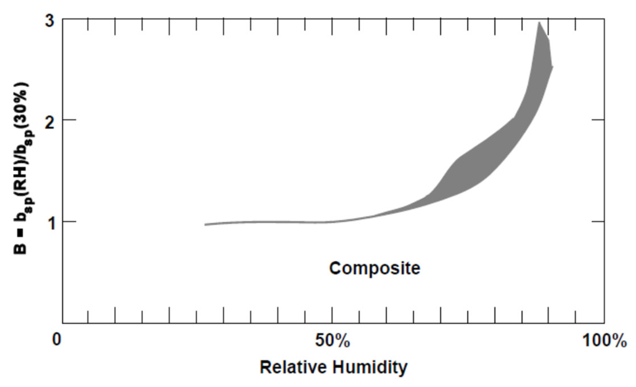
2.3. Humidity Adjustments

There are many factors that explain different outcomes between instrument types. Gravimetric samples continuously capture particles on a filter, nephelometer readings capture the degree of light scattered per second across the particles, and beta-attenuation readings capture the continuous absorption of radiation onto the particles [31]. The impact of humidity on these three instrument types is widely appreciated because particle size increases as the air becomes moist, thus affecting the results [39].
Table 1. General information about the study area.
ParishLand Area
(Square Miles)
Population
(2010 Census)
Adjusted Deaths
(May–Dec, 2010)
Jefferson296432,5521353
La Fourche106896,318300
Orleans169343,829559
Plaquemines78023,042-
St. Bernard37835,897-
Terrebonne1232111,860222
Region39231,043,4982434
Note: Death count is for persons aged 65 and over, adjusted for the number of days monitored. Adjusted deaths were approximately 90 percent of all deaths. The State of Louisiana and the CDC suppressed data for Plaquemines and St. Bernard Parishes due to low population. Sources: [40,41,42]. All data is public use.
Table 2. Summary of methods used.
Methods UsedLDEQ DataEPA Daily DataEPA Hourly DataCDC DataBP Data
Context of monitoringregulatoryemergencyemergencyresearchemergency
Monitoring typestationarystationarystationarymodelmobile
Monitoring locationurbancoastalcoastalregionalregional
Sample size (n)60086911442472101,262
Humidity calibration
Trend evaluation (graphical observation)
Normality evaluation (histogram, skew, kurtosis)
Centrality evaluation (mean, median)
Variability evaluation (mean absolute deviation, standard deviation, seasonal variation)
Comparison of peaks (short-term PM2.5 increases)
Sampling frequency analysis (samples per day compared to mean absolute deviation)
Comparison of means (t-tests)
Comparison of variances (F-tests)
Comparison of probability distributions (K-S tests)
Statistical power (Cohen’s D, effect size r, Hedge’s G)
Statistical relationship between variables (linear regression, multiple regression)
Multicollinearity analysis (tolerance test, variance inflation factor)
Abbreviations: LDEQ = Louisiana Department of Environmental Quality; EPA = US Environmental Protection Agency; CDC = US Centers for Disease Control and Prevention; BP = British Petroleum. Note: Only core findings are discussed in the text and depicted in subsequent tables and figures.
According to the EPA’s oil spill quality control plan [9], all PM2.5 data were controlled for humidity immediately upon obtaining each reading in comparison to a gravimetric sample. At the time, BP stated it was following EPA’s quality control plan, which applied to all sampling and monitoring for the disaster. Four years later, BP issued a data summary report that retroactively corrected for humidity, as follows:
“Personal aerosol monitors used for measuring PM2.5 and PM10 are significantly affected by humidity. At a relative humidity of 60%, the concentrations of PM2.5 and PM10 are overestimated by approximately 20%. At a relative humidity of 90%, the concentrations of PM2.5 and PM10 are overestimated by approximately 200%. Users should be aware that the relative humidity in the Gulf of Mexico region generally exceeds 60%; therefore, most of the results in the dataset are affected. Historic humidity readings can be obtained from the National Oceanic and Atmospheric Administration’s National Climatic Data Center.” [6].
Nephelometer overestimation typically begins at a humidity threshold of 60% [43,44,45,46] and peaks at about 90% [47,48], which defines the range of adjustment. To adjust BP’s PM2.5 data, historic humidity readings were obtained from NOAA [49] and all data points were transformed using the Covert et al. [47] and EPA [48] relationship (see Figure 2). This approach allowed more accurate adjustments because it extended the number of comparisons in between 60% and 90%.

2.4. Stationary and Modeled Data and Instruments

The stationary datasets available for comparison were: (1) Louisiana Department of Environmental Quality (LDEQ) “regulatory-stationary-urban” data taken routinely with permanent stationary gravimetric instruments and available to the public [10,24]; and (2) EPA’s “emergency-stationary-coastal” data taken with stationary Met One E-BAM beta-attenuation monitors only during the Gulf oil spill and available to the public [50]. A third dataset was the Centers for Disease Control and Prevention’s (CDC) “research-model-regional” results from its Downscaler Model for the period of the Gulf oil spill, developed in collaboration with the EPA and available to the public [7].
A sample of these three datasets is presented in Figure 3 to facilitate a side-by-side comparison to the mobile dataset. Figure 3 compares daily PM2.5 concentrations from August 21 to 6 September 2010 in Jefferson Parish and Plaquemines Parish. This timeframe was selected because it matched the dates of EPA’s hourly monitoring. All four of the datasets follow the same general trend at varying concentration levels. The graphs show that the CDC’s research-model-regional data and the LDEQ’s regulatory-stationary-urban data are consistently lower (in concentration) and smoother (fewer peaks) than the EPA’s emergency-stationary-coastal data and BP’s emergency-mobile-regional data. This is appropriate because research models and regulatory monitors are designed to produce normalized data for the purposes of predicting concentrations in locations without monitors and for comparison with regulatory standards. The emergency monitoring was not under these constraints; however, the EPA did follow conventional norms in establishing stationary monitors with hourly or daily time-controlled readings. The EPA monitors in Figure 3, however, were located along the coast and were positioned to capture any particulate matter blowing in from the spill, which might explain why they consistently produced the highest concentrations in concentrations in Figure 3. The BP emergency-mobile-regional data primarily lies in between the other datasets.

3. Results

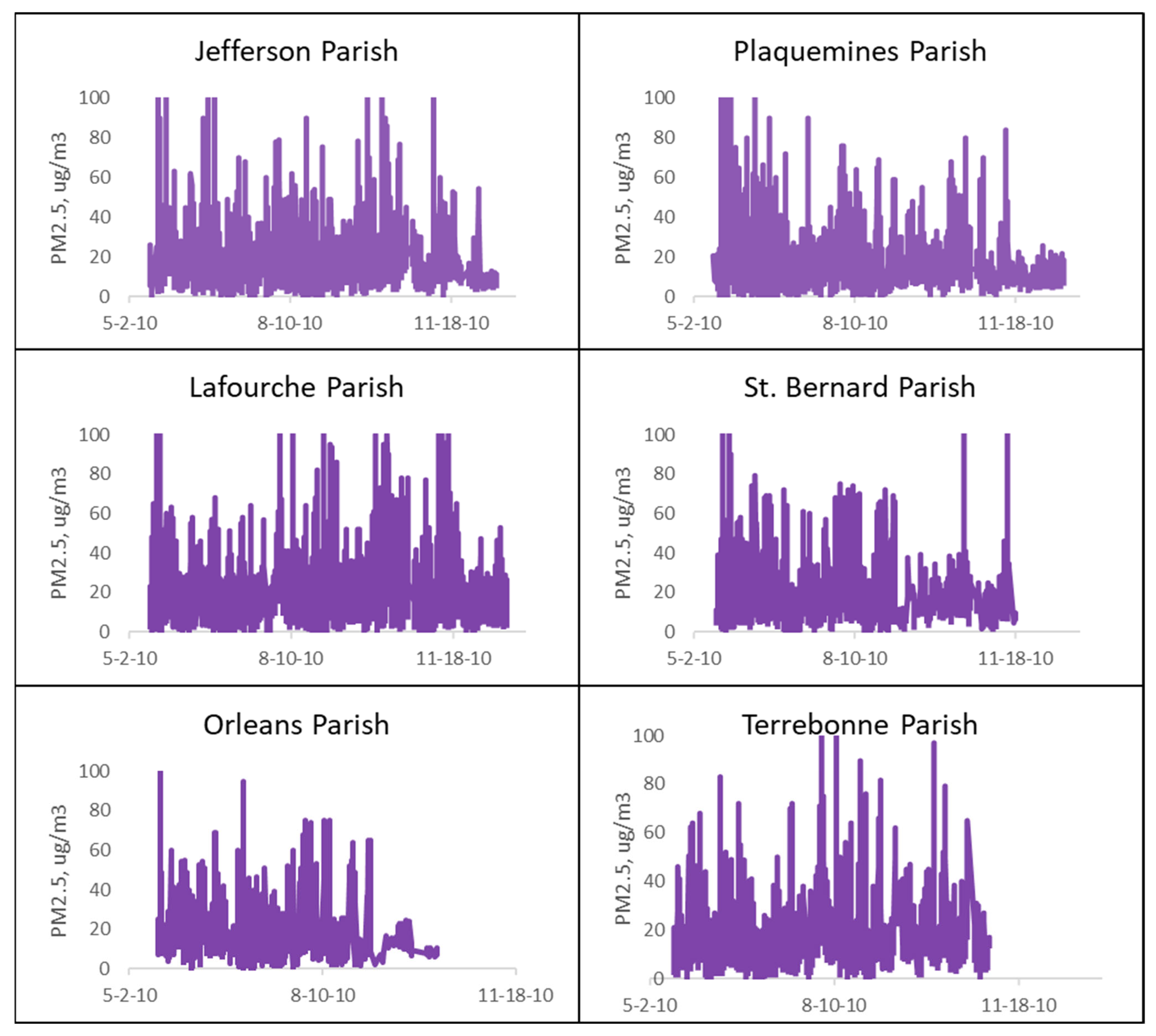
3.1. Data Variability

Two of the four available datasets were limited either in coverage area, duration, or number of samples. The LDEQ data only covered cities and took a total of 600 samples (every 1st, 3rd, or 6th day over 7 months) using stationary monitors in five of the six parishes, averaged on a 24-hour basis. The EPA data covered only the coastline and used stationary monitors to take either hourly or daily readings with sample sizes of 1144 (hourly over 17 days) and 869 (daily over five months) for the six parishes combined. While these two stationary datasets produced normalized data at points on the boundaries of the impacted region (the coastal edge and the urban areas), the data were not spatially or temporally representative of variability. For these reasons, these two datasets were deemed insufficient for an analysis of the association between variability and mortality. The CDC modeling dataset and the BP emergency dataset will be further assessed.
Figure 4 displays time series graphs of the BP emergency-mobile-regional data, corrected for humidity (parish sample size ranges from n = 4,682 to n = 32,968). The mean absolute deviation (MAD) ranges from 7.5 to 8.7 (overall MAD = 8.19), indicating high dispersion, numerous peaks or outliers, and variability that could be difficult to model or predict. Histograms confirmed that the distribution in each parish is log normal (skewness ranging from 1.55 to 17.60, kurtosis ranging from 5.73 to 985.2). The raw dataset is comprised of frequent, randomly timed readings that are spatially representative, with a relatively large total sample size (n = 101,262) and comprehensive spatial coverage (3923 acres) compared to the other datasets that were available. There are 4731 peaks above the 95th percentile, likely caused by a combination of the conditions of the oil spill, spatial variation, and unknown errors. However, the large sample size and approximately randomly timed readings reduces the impact of unknown errors. The conditions of the oil spill and spatial variation are part of the phenomenon that is represented by the dataset. Consequently, peaks were not considered outliers and were not removed because removing them would have distorted the results, as confirmed by Gorard [51] and Leys et al. [52]. Peaks were part of the situation being studied and reflect the variability of the event. Therefore, the median (13.60 μg/m3) was used instead of the mean to represent the central tendency.
Further evidence of high variability in the BP emergency-mobile-regional dataset can be seen by comparing peaks to exceedance days. For example, on 92 individual days between May and December 2010, Jefferson Parish (n = 19,106) had 1006 readings exceeding 35 μg/m3. During this same period, there were only three days with concentrations sustained enough to achieve a daily average that exceeded 35 μg/m3 (the daily National Ambient Air Quality Standard, NAAQS). Mobile monitoring generated many peaks but few consistently high concentrations, a pattern suggesting elevated short-lived peaks as identified by Russell [53]. All six parishes followed this pattern. This is an important finding because it confirms that a particulate matter distribution can simultaneously exhibit extremes of variability without extremes in daily average concentrations.
Figure 5 reveals seasonal variation in PM2.5 concentration for all six parishes, with increased concentrations in the spring and late summer/early fall. A similar pattern of higher PM2.5 concentrations in spring and fall was observed by Russell [53] in Southeast Texas. Chen et al. [54] found that seasonal variations in PM2.5 were associated with increased deaths in China.

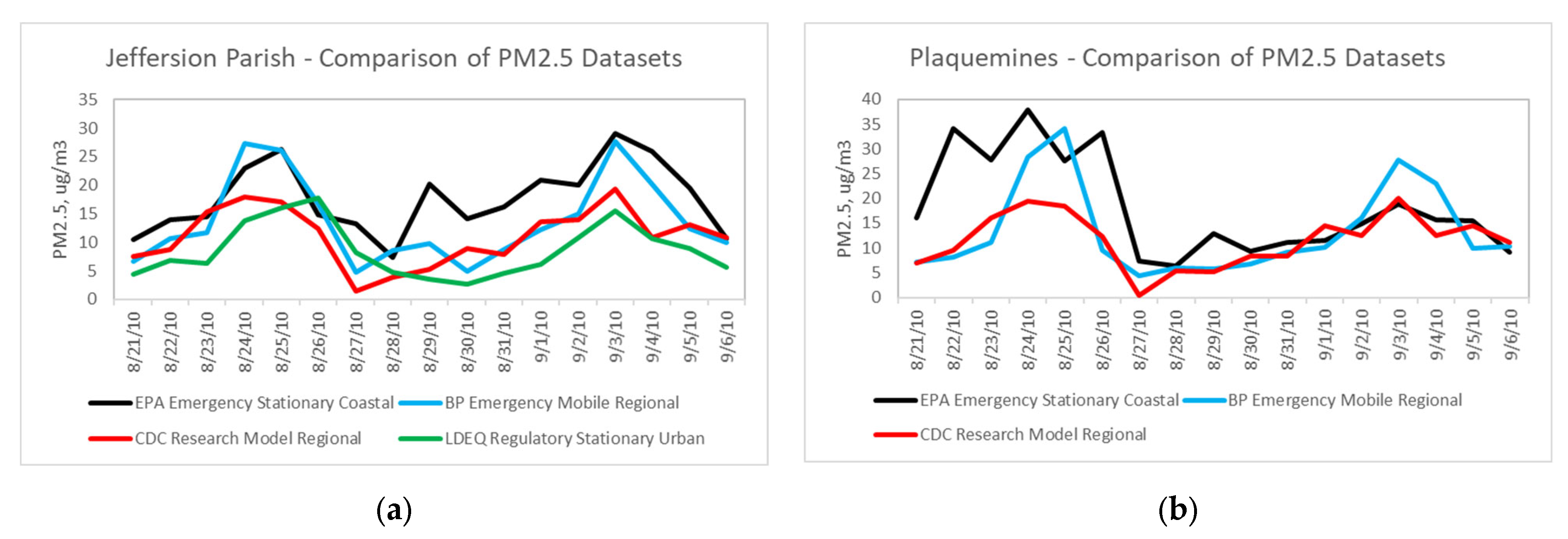
3.2. Modeled versus Mobile PM2.5 Data

The Downscaler statistical model was developed by the CDC in collaboration with EPA to predict PM2.5 concentrations in areas with low population and inadequate monitoring on the ground. The Downscaler model combines atmospheric model simulations with direct measurements of air pollution taken by 4000 nationwide regulatory monitors (including the LDEQ urban regulatory monitors). These results are part of the CDC’s National Environmental Health Tracking Network and are available to the public for use in environmental science and public health research [55]. Compared to the LDEQ and EPA datasets, the CDC model was the only dataset representing the entire region over the full duration of the disaster, with a robust sample size and more than one reading per day, making the CDC model results the best matching dataset for comparison to the BP mobile data. The model and mobile data were therefore directly compared.
When averaged by parish, the variability of the CDC’s research-model-regional distribution was much lower than the variability of BP’s emergency-mobile-regional distribution. An F-test on the variances confirmed a significant difference between the variances of the two distributions (ρ = 0.06, accept H0). However, a paired two-sample t-test on the means showed the means of the two distributions were equal (ρ = 0.39, two tail). Histograms of the modeled data were normally distributed (skewness = 0.97, kurtosis = 1.15), and the mobile data was normally skewed with a slightly high kurtosis (skewnes s = −1.44, kurtosis = 2.37). Values for skewness and kurtosis between −1.96 and +1.96 are considered acceptable to prove normal univariate distributions in MS Excel [56,57]. A Kolmogorov–Smirnov two-sample test revealed that these two samples did indeed come from the same distribution (D = 0.667, ρ = 0.143, α = 0.05). Overall, the comparison of parish averages finds that the mobile and modeled datasets are statistically similar in terms of PM2.5 concentration in the six parishes; however, the two datasets are statistically different in terms of variability [58].
Variability is the key difference between the modeled and mobile datasets. CDC’s modeled data consisted of two to three readings per day, while BP’s mobile data provided 3.7 readings per hour on average [6]. A higher number of readings captures more variability. Public health researchers have discovered that variability in PM2.5—measured as short-term increases of 10 μg/m3 or more—is directly associated with mortality in older populations [13]. Table 3 compares short-term increases (STI’s) in PM2.5 for the modeled and mobile data.
Table 3 demonstrates that variability is negligible in the modeled dataset, resulting in a trivial number of short-term increases (STIs). Despite the accuracy of the model data in terms of concentration and overall trends, it was not designed to capture the many changes in concentration that occurred in-between readings during the Gulf oil spill. In contrast, the mobile data took many thousands of readings and recorded more of the short-term increases that have been associated with death in older segments of the population. Using the mobile data, the remainder of the paper will directly test this association in the context of the Gulf oil spill.

3.3. Short-Term PM2.5 Increases and Mortality

The mobile dataset was analyzed for short term increases greater than or equal to 10 μg/m3 in preparation for analysis against mortality data. When the raw mobile data was aggregated into 7-day increments (to correspond to the 7-day mortality data that was available), it retained relatively high statistical power as indicated by a large Cohen’s D (1.939 > 0.8), a large effect size r (0.696 > 0.5); and a large Hedge’s G (1.833 > 0.8). Weekly mortality data was obtained from the Louisiana State Office of Health Statistics. In preparation for the analysis, deaths were counted proportionately based on the number of sampling days per week so that deaths that occurred on days without sampling were not included.
Researchers often incorporate a lag of one to five days between exposure and death, depending on the cause of death being studied. Such studies commonly use model results in which there are no missing data points, and many have access to daily mortality data. Several limitations of this study precluded the use of a lag between exposure and death. First, the data for this study are direct measurements of PM2.5 taken during a disaster. There was no data on some days, and this was random not systematic. Second, the region being studied has areas of low population so daily mortality data is not made available to the public; only weekly data are available. Third, the region has inadequate air pollution monitoring, and there is only one dataset available for analyzing correlations with mortality. Due to these circumstances, a lag analysis was not performed. Seven days of lag would likely be too long for all-cause mortality among persons 65 and older. A nationwide study of this cohort by Di et al. [13] used same-day and one-day prior exposure metrics and found high sensitivity and high mortality caused by exposure to PM2.5. This suggests that a short lag time would be needed to identify these deaths, but daily mortality data was not available so the question of lag time could not be addressed. Instead of adjusting deaths to a constant lag time, deaths were adjusted for miscellaneous days on which sampling did not occur, which amounted to 10 percent of all deaths during the study period. For the reasons stated above, this adjustment was considered more critical to the outcome of the analysis.
Ordinary least squares regression was performed using mortality data as the dependent variable versus short-term increases in PM2.5 as the independent variable, first by parish, then as multiple regression, and then disaggregated for the region. When analyzed individually using simple OLS regression, each parish had a significant relationship at the p < 0.05 level, but with small R-squared values ranging from 0.17–0.21, indicating a high degree of unaccounted for variation. When analyzed using multiple OLS regression, short-term particulate matter increases in all three parishes had a significant relationship with mortality (p < 0.05) with a moderate correlation (R2 = 0.51). Multicollinearity among the variables was checked by calculating tolerance levels and variance inflation factors (VIF) based on cutoff values established by Hair et al. [59]. Tolerance levels varied from 0.71–0.83, all exceeding the standard minimum of 0.2. VIFs varied from 1.20–1.41, all comfortably less than the maximum of 4.0. Therefore, the dataset did not have problems with multicollinearity.
In the final OLS regression analysis, all the raw data was blended to represent the region (i.e., not aggregated by parish). This run resulted in a strong statistically significant relationship (p < 0.001) and a moderate R-squared (R2 = 0.43). The full results are summarized in Table 4. There were positive, statistically significant relationships between PM2.5 and mortality no matter how the regression was done. Modeling the relationship at the regional scale gave the best results.
The analysis shows that short-term increases in fine particulate matter significantly and consistently predicted an increase in deaths throughout the study area from mid-May to mid-December, 2010, but with only moderate correlation. The deaths analyzed were all-cause deaths among people aged 65 and over in Jefferson, Lafourche, and Terrebonne Parishes. The overall finding of the study is that at the regional scale, each short-term increase of 10-μg/m3 or more of fine particulate matter was associated with a statistically significant increase of 0.105 all-cause deaths (p = 3.53E-5) in people aged 65 and over. This represents a 0.32% increase, which is in line with the findings of Kim et al. [15] who found statistically significant associations ranging from 0.18–0.32% for different causes of death.

4. Discussion

The analysis revealed that mobile monitoring during disasters is a critical supplement to existing stationary monitoring, which in Southeast Louisiana does not fully represent spatial and temporal variability. The mobile monitoring made it possible to observe frequent short-lived peaks for many consecutive months, data that was missed by the other three datasets that were available during the disaster. This data gap was linked to important public health risks, including mortality in sensitive groups.
Emergency stationary monitors installed by EPA along the coast picked up the highest PM2.5 concentrations coming in from the offshore spill. However, these daily and hourly data lacked spatial resolution, and the hourly sampling was only operated for a brief 17-day period, so both daily and hourly emergency datasets lacked the spatiotemporal resolution needed to assess mortality. Daily PM2.5 concentrations were simultaneously gathered at six regulatory monitors located in the urban centers and regulated by LDEQ. While these data were continuous throughout the year, only daily averages were made available to the public, and these failed to measure short term increases in between readings. The LDEQ data were also stationary and therefore lacked spatial resolution. The CDC model provided long term spatially integrated data, but with only two or three data points per day, which again missed peaks in between readings. The analysis found that the CDC’s model results aligned well with BP’s emergency monitoring data in terms of concentration and overall trend; however, the modeled output was much less variable than the real-time data, so it missed most of the short-term increases in PM2.5 that occurred during the disaster.
None of the usual monitoring in Southeast Louisiana made it possible to measure the association between particulate matter and mortality because of the ways in which monitoring was carried out, yet all the usual monitoring complied with National Ambient Air Quality Standards. This suggests that the current regulatory regime tolerates particulate matter deaths both during disasters and during normal times, and that current policies are not health protective.
In response to the first research question, (1) Compared to other available data, was spatiotemporal data better at representing PM2.5 variability during the Gulf oil spill?, evaluation of all available datasets during the Gulf oil spill confirmed that the spatiotemporal mobile monitoring dataset was the only suitable dataset for analyzing PM variability. The second research question, (2) Were deaths during the Gulf oil spill in people aged 65 and over associated with PM2.5 variability?, was addressed using OLS regressions of mortality versus short-term increases in PM2.5 within the study area and timeframe. The analysis identified a statistically significant relationship between short-term increases of PM2.5 and mortality in elders 65 and over, a finding that aligns with other recently published research on mortality and fine particulate matter [13,15,60].
It is likely that BP’s mobile monitoring data contained too much unnecessary variation. BP’s monitoring scheme took an 8-month average of 3.7 readings per hour over 89,982 linear miles and 31 readings per square mile. These are impressive numbers, but the low R-squared values are likely due to excess variation in the data. One way to estimate this would be to examine the relationship between sampling frequency and variability. The datasets that averaged 2.2 readings per day (LDEQ, CDC, and EPA daily) measured a limited amount of particulate matter variability, as indicated by an average mean absolute deviation (MAD) of 4.4. In contrast, the datasets with a median of 2.4 readings per hour (BP and EPA hourly) had a mean absolute deviation (MAD) of 8.9. Frequent monitoring leads to more accurate variability, which facilitates the identification of short-term increases that may be statistically associated with mortality. The EPA hourly monitoring frequency was high enough to capture variability, but as mentioned previously, the two-week monitoring duration did not catch enough short-term increases in PM2.5 to support a statistical analysis with mortality. BP’s overall sampling frequency of 3.7 per hour, combined with its spatial representation and long duration, ensured a full picture of PM2.5 variability and a robust set of short-term increases that could be statistically analyzed against deaths. Based on comparison with the other available datasets, mobile monitoring could have captured less data and still obtained results adequate for showing the PM-mortality relationship. An average sampling frequency of 2.4 readings per hour with a MAD variability of 7.5 or higher may have been adequate. This is an interesting research question that deserves further study.
From analyzing the other datasets that were taken at the same time and location as the mobile dataset, it was apparent that daily and hourly readings were not frequent enough, and that the two-week coastal monitoring period needed to be much longer. The lack of spatial variation was also problematic. In the conventional monitoring regimes examined in this research, too much particulate matter variation went unmonitored and the monitoring results that were obtained were unable to identify statistically significant associations with mortality. The computer modelling that was produced by the CDC using conventional data produced only a couple of concentration values per day and these results, while valuable for tracking concentration, stopped short of providing insights into variability, which causes death. In contrast, the mobile monitors had the advantage of taking nearly random readings rather than on-the-hour readings, and because of the long duration of monitoring it produced a quasi-random sample, which was more representative of what the population actually breathed.
This research has exposed a number of gaps in knowledge that can be addressed in future research: (1) what is the ideal monitoring rate (readings per hour) for capturing an effective amount of variability?; (2) what is the minimum duration of monitoring to capture enough data to support a statistical comparison to public health data?; and (3) is the body of evidence—including this and many other papers on the subject—persuasive enough to make air pollution regulations more protective of public health?

5. Conclusions

During the Gulf oil spill, fine particulates traveled into a region containing a large population known to have disproportionately high underlying disease burden [61]. These emissions affected air quality on a regional basis. The most likely PM sources were vehicle emissions caused by increased car, truck, and boat traffic during the disaster, controlled burns for reducing floating contaminants, direct emissions from the oil spill, and secondary generation of aerosols from the oil spill (precursors). These sources did not create consistent emissions from a single location or of a single type; rather, they produced transient emissions from multiple sources and created multiple points of exposure. These conditions led to increased variability in PM2.5 during the disaster, as demonstrated by the spatiotemporal monitoring analyzed in this paper. Routine regulatory monitoring, and emergency monitoring based on routine monitoring norms (i.e., hourly or daily readings, stationary monitors, short durations, normalization of data), failed to recognize variability that was linked to public health. Computer models that followed these same norms were unable to represent variability.
This paper has demonstrated that short term increases in PM2.5 were associated with all-cause mortality in people over the age of 65 in the region impacted by the Gulf oil spill. These findings have implications for environmental policy and for disaster management. In the case of the Gulf oil spill, this paper has demonstrated the importance of capturing spatial and temporal dimensions in ambient air monitoring. When emissions are not controlled or predictable, such as during a disaster, spatially and temporally integrated monitoring at frequencies greater than once per hour and for long durations are essential for capturing data relevant to public health. Spatiotemporal approaches to monitoring and modelling can reveal far more of the variability that exists during air pollution disasters and can be a robust source of data for understanding the impacts of fine particulate matter on mortality.

Funding

This research received no external funding.

Institutional Review Board Statement

Not applicable.

Informed Consent Statement

Not applicable.

Data Availability Statement

The data that support the findings of this study are publicly available in the Gulf of Mexico Research Initiative at https://gulfresearchinitiative.org/ (accessed on 18 March 2021), doi:10.7266/N7BR8QMW, reference number BP.x750.000:0024; and in the Louisiana State Center for Health Statistics, by request at https://ldh.la.gov/index.cfm/form/80 (accessed on 18 March 2021).

Acknowledgments

The author acknowledges the U.S. Environmental Protection Agency and British Petroleum for making their real-time disaster monitoring data available. The author also acknowledges the Louisiana State Center for Health Statistics for providing mortality data.

Conflicts of Interest

The author declares no conflict of interest.

References

  1. Zhu, K.; Zhang, J.; Lioy, P. Evaluation and Comparison of Continuous Fine Particulate Matter Monitors for Measurement of Ambient Aerosols. J. Air Waste Manag. Assoc. 2007, 57, 1499–1506. [Google Scholar] [CrossRef] [PubMed] [Green Version]
  2. National Commission on the BP Deepwater Horizon Oil Spill and Offshore Drilling. Deep Water: The Gulf Oil Disaster and the Future of Offshore Drilling, A Report to the President. January 2011. Available online: https://www.govinfo.gov/content/pkg/GPO-OILCOMMISSION/pdf/GPO-OILCOMMISSION.pdf (accessed on 18 March 2021).
  3. De Gouw, J.A.; Middlebrook, A.M.; Warneke, C.; Ahmadov, R.; Atlas, E.L.; Bahreini, R.; Blake, D.R.; Brock, C.A.; Brioude, J.; Fahey, D.W.; et al. Organic Aerosol Formation Downwind from the Deepwater Horizon Oil spill. Science 2011, 331, 1295. [Google Scholar] [CrossRef] [PubMed] [Green Version]
  4. Middlebrook, A.; Murphy, D.; Ahmadov, R.; Atlas, E.; Bahreini, R.; Blake, D.; Brioude, J.; Gouw, J.D.; Fehsenfeld, F.; Frost, G.; et al. Air Quality Implications of the Deepwater Horizon Oil spill. Proc. Natl. Acad. Sci. USA 2012, 109, 20280–20285. [Google Scholar] [CrossRef] [PubMed] [Green Version]
  5. National Oceanic and Atmospheric Administration. Insights from Oil Spill Air Pollution Study Have Implications Beyond Gulf. 11 March 2011. Available online: https://csl.noaa.gov/news/2011/92_0311.html (accessed on 20 January 2021).
  6. British Petroleum. Data Publication Summary Report: Community Air Sampling and Monitoring Data. Reference No. OTH-04v01-02. 2014. Available online: https://data.gulfresearchinitiative.org/data/BP.x750.000:0024 (accessed on 20 April 2019).
  7. Centers for Disease Control and Prevention. Monitor + Model Air Data. National Environmental Public Health Tracking. 2019. Available online: https://ephtracking.cdc.gov/showAirMonModData (accessed on 20 January 2021).
  8. Environmental Protection Agency. Final Rule on the Implementation of the New Source Review Provisions for Particulate Matter Less Than 2.5 Microns (PM2.5); 77 FR 65107; U.S. Environmental Protection Agency: Washington, DC, USA, 2012. Available online: https://www.epa.gov/sites/production/files/2015-12/documents/20080508_fs.pdf (accessed on 25 December 2020).
  9. Environmental Protection Agency. Quality Assurance Sampling Plan for British Petroleum Oil Spill. 2010. Available online: https://archive.epa.gov/emergency/bpspill/web/pdf/appendixe-data_management_plan_5-30.pdf (accessed on 20 April 2019).
  10. Louisiana Department of Environmental Quality. Ambient Air Monitoring Stations. 2011. Available online: https://www.deq.louisiana.gov/page/ambient-air-monitoring-data-reports (accessed on 20 November 2013).
  11. Nance, E.; King, D.; Wright, B.; Bullard, R.D. Ambient air concentrations exceeded health-based standards for fine particulate matter and benzene during the Deepwater Horizon oil spill. J. Air Waste Manag. Assoc. 2016, 66, 224–236. [Google Scholar] [CrossRef] [PubMed]
  12. Air Now. Air Quality Index (AQI)—A Guide to Air Quality and Your Health. 2013. Available online: http://airnow.gov/index.cfm?action=aqibasics.aqi (accessed on 5 October 2013).
  13. Di, Q.; Dai, L.; Wang, Y.; Zanobetti, A.; Choirat, C.; Schwartz, J.D.; Dominici, F. Association of short-term exposure to air pollution with mortality in older adults. JAMA 2017, 318, 2446–2456. [Google Scholar] [CrossRef]
  14. Schwartz, J. Air Pollution and Daily Mortality: A Review and Meta Analysis. Environ. Res. 1994, 64, 36–52. [Google Scholar] [CrossRef]
  15. Kim, S.E.; Hijioka, Y.; Nagashima, T.; Kim, H. Particulate Matter and Its Impact on Mortality among Elderly Residents of Seoul, South Korea. Atmosphere 2020, 11, 18. [Google Scholar] [CrossRef] [Green Version]
  16. Staniswalis, J.G.; Parks, N.J.; Bader, J.O.; Maldonado, Y.M. Temporal Analysis of Airborne Particulate Matter Reveals a Dose-Rate Effect on Mortality in El Paso: Indications of Differential Toxicity for Different Particle Mixtures. J. Air Waste Manag. Assoc. 2005, 55, 893–902. [Google Scholar] [CrossRef] [Green Version]
  17. Krudysz, M.; Moore, K.; Geller, M.; Sioutas, C.; Froines, J. Intra-community Spatial Variability of Particulate Matter Size Distributions in Southern California/Los Angeles. Atmos. Chem. Phys. 2009, 9, 1061–1075. [Google Scholar] [CrossRef] [Green Version]
  18. Zhu, Y.; Hinds, W.C.; Kim, S.; Sioutas, C. Concentration and Size Distribution of Ultrafine Particles near a Major Highway. J. Air Waste Manag. Assoc. 2002, 52, 1032–1042. [Google Scholar] [CrossRef] [PubMed]
  19. Peters, J.; Theunis, J.; Van Poppel, M.; Berghmans, P. Monitoring PM10 and Ultrafine Particles in Urban Environments Using Mobile Measurements. Aerosol Air Qual. Res. 2013, 13, 509–522. [Google Scholar] [CrossRef]
  20. Gulev, S.K. Climatologically significant effects of space–time averaging in the North Atlantic sea–air heat flux fields. J. Clim. 1997, 10, 2743–2763. [Google Scholar] [CrossRef] [Green Version]
  21. Hughes, P.J.; Bourassa, M.A.; Rolph, J.J.; Smith, S.R. Averaging-Related Biases in Monthly Latent Heat Fluxes. J. Atmos. Ocean. Technol. 2012, 29, 974–986. [Google Scholar] [CrossRef]
  22. Kaiser, J. Epidemiology. How dirty air hurts the heart. Science 2005, 307, 1858–1859. [Google Scholar] [CrossRef]
  23. Conroy, D.; McWilliams, A. Challenges and Issues with Reporting the AQI for PM2.5 on a Real-time Basis (slides). Environmental Protection Agency. 2001. Available online: https://slideplayer.com/slide/4160546/ (accessed on 20 March 2021).
  24. Environmental Protection Agency. Outdoor Air Quality Data. 2020. Available online: https://www.epa.gov/outdoor-air-quality-data (accessed on 22 December 2020).
  25. Yuval, D.M.; Broday, Y.C. Mapping spatiotemporal variables: The impact of the time-averaging window width on the spatial accuracy. Atmos. Environ. 2005, 39, 3611–3619. [Google Scholar] [CrossRef]
  26. Evangelista, M. Investigation of 1-hour PM2.5 Mass Concentration Data from EPA-Approved Continuous Federal Equivalent Method Analyzers. Environmental Protection Agency Office of Air Quality Planning and Standards. 2011. Available online: https://www3.epa.gov/ttn/naaqs/standards/pm/data/Evangelista040511.pdf (accessed on 20 December 2013).
  27. Steinle, S.; Reis, S.; Sabel, C.E. Quantifying human exposure to air pollution—Moving from static monitoring to spatiotemporally resolved personal exposure assessment. Sci. Total Environ. 2013, 443, 184–193. [Google Scholar] [CrossRef] [Green Version]
  28. Perring, A.E.; Schwarz, J.P.; Spackman, J.R.; Bahreini, R.; de Gouw, J.A.; Gao, R.S.; Holloway, J.S.; Lack, D.A.; Langridge, J.M.; Peischl, J.; et al. Characteristics of Black Carbon Aerosol from a Surface Oil Burn During the Deepwater Horizon Oil spill. Geophys. Res. Lett. 2011, 38, 17. [Google Scholar] [CrossRef]
  29. Kumar, P.; Morawska, L.; Birmili, W.; Paasonen, P.; Hu, M.; Kulmala, M.; Harrison, R.M.; Norford, L.; Britter, R. Ultrafine particles in cities. Environ. Int. 2014, 66, 1–10. [Google Scholar] [CrossRef] [Green Version]
  30. Sabaliauskas, K.; Jeong, C.H.; Yao, X.; Jun, Y.S.; Jadidian, P.; Evans, G.J. Five-year roadside measurements of ultrafine particles in a major Canadian city. Atmos. Environ. 2012, 49, 245–256. [Google Scholar] [CrossRef]
  31. Heal, M.R.; Kumar, P.; Harrison, R.M. Particles, air quality, policy and health. Chem. Soc. Rev. 2012, 41, 6606–6630. [Google Scholar] [CrossRef] [Green Version]
  32. Birmili, W.; Tomsche, L.; Sonntag, A.; Opelt, C.; Weinhold, K.; Nordmann, S.; Schmidt, W. Variability of aerosol particles in the urban atmosphere of Dresden (Germany). Effects of spatial scale and particle size. Meteorol. Z. 2013, 22, 195–211. [Google Scholar] [CrossRef]
  33. Costabile, F.; Birmili, W.; Klose, S.; Tuch, T.; Wehner, B.; Wiedensohler, A.; Franck, U.; König, K.; Sonntag, A. Spatiotemporal variability and principal components of the particle number size distribution in an urban atmosphere. Atmos. Chem. Phys. 2009, 9, 3163–3195. [Google Scholar] [CrossRef] [Green Version]
  34. Ross, Z.; Ito, K.; Johnson, S.; Yee, M.; Pezeshki, G.; Clougherty, J.E.; Savitz, D.; Matte, T. Spatial and temporal estimation of air pollutants in New York City: Exposure assignment for use in a birth outcomes study. Environ. Health 2013, 12, 1–13. Available online: http://www.ehjournal.net/content/12/1/51 (accessed on 11 July 2014). [CrossRef] [PubMed] [Green Version]
  35. Peres, L.C.; Trapido, E.; Rung, A.L.; Harrington, D.J.; Oral, E.; Fang, Z.; Fontham, E.; Peters, E.S. The Deepwater Horizon Oil Spill and Physical Health among Adult Women in Southern Louisiana: The Women and Their Children’s Health (WaTCH) Study. Environ. Health Perspect. 2016, 124, 1208–1213. [Google Scholar] [CrossRef] [Green Version]
  36. Centers for Disease Control and Prevention. FastStats: Older Persons’ Health. National Center for Health Statistics. 2021. Available online: https://www.cdc.gov/nchs/fastats/older-american-health.htm (accessed on 15 February 2021).
  37. GIS Geography. Open Source Louisiana Parish Map. 2021. Available online: https://gisgeography.com/louisiana-parish-map/ (accessed on 23 March 2021).
  38. Environmental Protection Agency. List of Designated Reference and Equivalent Methods. Office of Research and Development. 2014. Available online: www.epa.gov/ttn/amtic/criteria.html (accessed on 28 July 2014).
  39. Hernandez, G.; Berry, T.-A.; Wallis, S.L.; Poyner, D. Temperature and Humidity Effects on Particulate Matter Concentrations in a Sub-Tropical Climate During Winter. Proc. Int. Conf. Environ. Chem. Biol. 2017, 102, 41–49. [Google Scholar] [CrossRef]
  40. Index Mundi. Louisiana Land Area in Square Miles, 2010 by County. 2019. Available online: https://www.indexmundi.com/facts/united-states/quick-facts/louisiana/land-area#map (accessed on 24 February 2019).
  41. U.S. Census Bureau. County Population Totals: 2010–2019. 2020. Available online: https://www.census.gov/data/tables/time-series/demo/popest/2010s-counties-total.html (accessed on 1 February 2021).
  42. Louisiana State Center for Health Statistics. Louisiana State Office of Public Health, New Orleans, LA. (Data by Request, Received on 4 February 2021). Available online: https://ldh.la.gov/index.cfm/page/647 (accessed on 25 January 2021).
  43. Soneja, S.; Chen, C.; Tielsch, J.M.; Katz, J.; Zeger, S.L.; Checkley, W.; Curriero, F.C.; Breysse, P.N. Humidity and gravimetric equivalency adjustments for nephelometer-based particulate matter measurements of emissions from solid biomass fuel use in cookstoves. Int. J. Environ. Res. Public Health 2014, 11, 6400–6416. [Google Scholar] [CrossRef] [PubMed] [Green Version]
  44. Wu, Z.; Bo, H.; Changhe, C.; Ping, D.; Lei, Z.; Guanghong, F. Scattering properties of atmospheric aerosols over Lanzhou City and applications using an integrating nephelometer. Adv. Atmos. Sci. 2004, 21, 848–856. [Google Scholar] [CrossRef]
  45. Sioutas, C.; Kim, S.; Chang, M.; Terrell, L.L.; Gong, H., Jr. Field evaluation of a modified DataRAM MIE scattering monitor for real-time PM2. 5 mass concentration measurements. Atmos. Environ. 2000, 34, 4829–4838. [Google Scholar] [CrossRef]
  46. Chakrabarti, B.; Fine, P.M.; Delfino, R.; Sioutas, C. Performance evaluation of the active-flow personal DataRAM PM2. 5 mass monitor (Thermo Anderson pDR-1200) designed for continuous personal exposure measurements. Atmos. Environ. 2004, 38, 3329–3340. [Google Scholar] [CrossRef]
  47. Covert, D.S.; Waggoner, A.P.; Weiss, R.E.; Ahlquist, N.C.; Charlson, R.J. Atmospheric aerosols, humidity, and visibility. In The Character and Origins of Smog Aerosols: A Digest of Results from the California Aerosol Characterization Experiment (ACHEX); Advances in Environmental Science and Technology: V. 9; Hidy, G.M., Mueller, P.K., Grosjean, D., Appel, B.R., Wesolowski, J.J., Eds.; John Wiley & Sons, Inc.: New York, NY, USA, 1980; pp. 559–581. [Google Scholar]
  48. Environmental Protection Agency. Air Quality Criteria for Particulate Matter; EPA/600/P-95/001bF; Office of Research and Development: Washington, DC, USA, 1996; Volume II of III. [Google Scholar]
  49. National Oceanic and Atmospheric Administration. National Centers for Environmental Information (formerly National Climatic Data Center). Available online: https://www.ncdc.noaa.gov/cdo-web/ (accessed on 20 December 2020).
  50. Environmental Protection Agency. EPA Response to the BP Oil Spill in the Gulf of Mexico. 2013. Available online: https://archive.epa.gov/emergency/bpspill/web/html/epa.html (accessed on 27 May 2015).
  51. Gorard, S. Revisiting a 90-year-old debate: The advantages of the mean deviation. Br. J. Educ. Stud. 2005, 53, 417–430. [Google Scholar] [CrossRef]
  52. Leys, C.; Delacre, M.; Mora, Y.L.; Lakens, D.; Ley, C. How to classify, detect, and manage univariate and multivariate outliers, with emphasis on pre-registration. Int. Rev. Soc. Psychol. 2019, 32, 1–10. [Google Scholar] [CrossRef]
  53. Russell, M.; Allen, D.T.; Collins, D.R.; Fraser, M.P. Daily, Seasonal, and Spatial Trends in PM2.5 Mass and Composition in Southeast Texas Special Issue of Aerosol Science and Technology on Findings from the Fine Particulate Matter Supersites Program. Aerosol Sci. Technol. 2004, 38, 14–26. [Google Scholar] [CrossRef] [Green Version]
  54. Chen, R.; Peng, R.D.; Meng, X.; Zhou, Z.; Chen, B.; Kan, H. Seasonal variation in the acute effect of particulate air pollution on mortality in the China Air Pollution and Health Effects Study (CAPES). Sci. Total Environ. 2013, 450–451, 259–265. [Google Scholar] [CrossRef] [Green Version]
  55. Centers for Disease Control and Prevention. Air Quality Measures on the National Environmental Health Tracking Network. 2018. Available online: https://data.cdc.gov/Environmental-Health-Toxicology/Air-Quality-Measures-on-the-National-Environmental/cjae-szjv (accessed on 20 March 2021).
  56. George, D.; Mallery, M. SPSS for Windows Step by Step: A Simple Guide and Reference, 10th ed.; 17.0 Update; Pearson: Boston, MA, USA, 2010. [Google Scholar]
  57. Gravetter, F.; Wallnau, L. Essentials of Statistics for the Behavioral Sciences, 8th ed.; Belmont, CA: Wadsworth, OH, USA, 2014. [Google Scholar]
  58. Ghasemi, A.; Zahediasl, S. Normality Tests for Statistical Analysis: A Guide for Non-Statisticians. Int. J. Endocrinol. Metab. 2012, 10, 486–489. [Google Scholar] [CrossRef] [Green Version]
  59. Hair, J.F., Jr.; Babin, B.; Anderson, R.E. Multivariate Analysis: A Global Perspective; Kennesaw State University: Kennesaw, GA, USA, 2010. [Google Scholar]
  60. Liu, Y.; Pan, J.; Zhang, H.; Shi, C.; Li, G.; Peng, Z.; Ma, J.; Zhou, Y.; Zhang, L. Short-term exposure to ambient air pollution and asthma mortality. Am. J. Respir. Crit. Care Med. 2019, 200, 24–32. [Google Scholar] [CrossRef] [Green Version]
  61. Goldstein, B.D.; Osofsky, H.J.; Lichtveld, M.Y. The Gulf Oil Spill. N. Engl. J. Med. 2011, 364, 1334–1348. [Google Scholar] [CrossRef] [Green Version]
Figure 1. Terrestrial mobile air monitoring routes in six Southeast Louisiana parishes. Readings taken over water by boat were not included in the analysis. Sources: Public use data from BP [6]; public use map by GIS Geography [37]; and map enhancements by Angel Torres.
Atmosphere 12 00420 g001
Figure 2. Dependence of the light-scattering coefficient of ambient aerosol on relative humidity in various areas of the United States [47,48].
Atmosphere 12 00420 g002
Figure 3. (a,b) Comparison of a sample of datasets taken during the Gulf oil spill. Note that Plaquemines Parish has no regulatory monitors due to low population levels; data was only available for Plaquemines because of emergency monitoring and subsequent modeling. Sources: [6,7,10,24,50]. All data is public use.
Atmosphere 12 00420 g003
Figure 4. Time series graphs of raw PM2.5 data in the 6-parish region during the Gulf oil spill, gathered by mobile monitors. Source: Public use data from BP [6].
Atmosphere 12 00420 g004
Figure 5. Trends in PM2.5 concentration, aggregated by month and by parish, during the Gulf oil spill. Higher concentrations occurred in spring and late summer/early fall. (n = 44). Source: Public use data from BP [6].
Atmosphere 12 00420 g005
Table 3. Comparison of centrality (mean, median) and variability (STI) in the modeled and mobile datasets, by parish and for the region.
Modeled DataMobile Data
Sample
Size, n
Mean
μg/m3
Median
μg/m3
Short-term
Increases
STI
Sample
Size, n
Mean
μg/m3
Median
μg/m3
Short-term
Increases
STI
Jefferson40313.0313.03319,10615.9713.501932
Lafourche56312.8713.03332,96717.2814.404290
Orleans22313.1312.783468117.4514.50722
Plaquemines57213.3813.20218,47814.6412.002029
St. Bernard32013.9513.88310,25516.6213.601140
Terrebonne39112.7512.89215,77516.6214.001477
Region247213.2213.1816101,26216.3913.6011,590
Note: STI = short term increases in PM2.5 ≥ 10 μg/m3. Time period is May–December 2010. Sources: [6,7]. All data is public use.
Table 4. Association of All-Cause Mortality with Short-Term Increases in PM2.5.
OLS RegressionnRR2Adj. R2SEβρ95% CI
Simple
Jefferson310.460.210.1814.370.17990.0096 **(0.05,0.31)
Lafourche330.440.190.163.4850.01640.0113 *(0.00,0.03)
Terrebonne260.410.170.133.2480.03260.0326 *(0.00,0.06)
Multiple330.710.510.4616.09
Jefferson 0.16790.0443 *(0.01,0.33)
Lafourche 0.06320.0496 *(0.00,0.13)
Terrebonne 0.18680.0116 *(0.04,0.33)
Simple
Unaggregated330.660.430.4116.770.10463.53E-5 ***(0.06,0.15)
Note: alpha = 0.05. n = weeks sampled. All-cause mortality data is weekly, for persons aged 65 and over. Data for the remaining parishes was insufficient because BP’s monitoring in Orleans Parish was much shorter than the other parishes, and because the CDC suppressed mortality data for Plaquemines and St. Bernard Parishes due to low population. * p < 0.05; ** p < 0.01; *** p < 0.001.
Publisher’s Note: MDPI stays neutral with regard to jurisdictional claims in published maps and institutional affiliations.

