Features Exploration from Datasets Vision in Air Quality Prediction Domain
Abstract
1. Introduction
2. Methods
3. Results and Discussion
4. Conclusions
Author Contributions
Funding
Institutional Review Board Statement
Informed Consent Statement
Data Availability Statement
Conflicts of Interest
Appendix A
| Work | Year | Case Study | Prediction Target | Dataset Type | Data Rate | Period (Days) | Open Data | Algorithm | Time Granularity | Evaluation Metric |
|---|---|---|---|---|---|---|---|---|---|---|
| [36] | 2020 | USA | PM2.5 | Spatial, Temporal, AOD, PBL Height | Daily | 5779 | No | Hybrid | 24 h | RMSE, SD, R2 |
| [50] | 2020 | Canada | UFP | MET, Traffic, Land Use, BEV | N/S | 120 | No | Ensemble | RMSE, R2 | |
| [51] | 2020 | Taiwan | PM2.5, PM10 | MET | N/S | 2192 | No | Hybrid | 8 h | RMSE, MAE |
| [39] | 2020 | China | PM2.5, NOx | MET, Traffic | Hourly | 731 | No | Regression, Ensemble | 1 h | RMSE, ME, NRMSE, NME, POD, POF, R2 |
| [21] | 2020 | USA | PM2.5 | MET, Temporal | Hourly | 730 | No | NN | RMSE, MAE, MAPE | |
| [42] | 2020 | India | PM2.5 | MET | Hourly | 1230 | No | NN | RMSE, R2 | |
| [52] | 2020 | USA | AQI | MET | Hourly | 851 | Yes | Regression | 1 h | RMSE, MAE, NRMSE, R |
| [53] | 2020 | Turkey | PM10 | Spatial, Land Use | N/S | 3652 | No | Regression, Ensemble, NN | RMSE, MAE, R2 | |
| [54] | 2020 | China | PM2.5 | MET | Hourly | 31 | Yes | NN | 1 h | RMSE, R |
| [55] | 2020 | China | AQHI, IAQL | MET, Temporal | Hourly | 730/1826 | Yes | Ensemble | 12 h | Acc, MSE, WP, WR, WF |
| [56] | 2020 | China | PM10 | MET | Daily | 1096 | No | NN | 24 h | RMSE, ME, R, EOp |
| [37] | 2020 | Tunisia, Italy | MET, Temporal | Hourly | 1461/366 | No | Ensemble | 1 week | aRRMSE, aRMSE, R2, aCC, MSE, aRE, RP | |
| [38] | 2020 | China | PM2.5 | MET | N/S | 46 | Yes | Ensemble | 24 h | RMSE, MAE, SMAPE |
| [41] | 2020 | China | PM2.5 | MET | Hourly | 1825 | No | NN | 1 week | RMSE |
| [57] | 2020 | China | PM2.5 | MET | N/S | 1096 | Yes | NN | 24 h | RMSE, MAE, MAPE |
| [46] | 2020 | China | O3 | MET, UV Index | Daily | 1491 | Yes | Hybrid | 1 week | RMSE, MAE, MAPE, IA |
| [58] | 2020 | South Korea | PM2.5, PM10 | MET | Hourly | 1461 | Yes | Hybrid | 15days | RMSE, MAE |
| [40] | 2020 | China | PM2.5, PM10, NO2, NO, CO | MET | Daily | 4656 | No | NN | 24 h | MSE |
| [59] | 2020 | Taiwan | PM2.5 | MET, Spatial, Temporal | Hourly | 365 | Yes | Ensemble | 24 h | RMSE, NRMSE, R2 |
| [60] | 2020 | UK | PM2.5 | MET, Spatial, Temporal, AOD, Land Use | Daily | 3287 | Partially | Ensemble | 24 h | RMSE, MSE, R2 |
| [61] | 2020 | Ecuador | PM2.5 | MET, Spatial, Temporal, Traffic | 5 s | 4 | No | Other Algorithms | Acc | |
| [62] | 2020 | China | PM2.5 | MET | Hourly | 365 | No | Ensemble | 48 h | MSE, IA, NMGE, R2 |
| [63] | 2020 | China | PM2.5 | MET | Hourly | 1461 | No | Ensemble | 24 h | RMSE, MB, ME, R |
| [64] | 2020 | China | AQI | MET | Hourly | 2192 | No | NN | 48 h | RMSE, Acc |
| [32] | 2020 | China | AQI | MET | Hourly | 730 | Yes | NN | 24 h | RMSE, MAE, R2, FB |
| [65] | 2020 | South Korea | PM2.5, PM10 | MET, Temporal, Spatial | Minutely | 7 | No | Hybrid | RMSE | |
| [66] | 2020 | China | PM2.5, PM10, O3, NO2, SO2, CO | MET, Social Media | Daily | 731 | Yes | NN | 24 h | RMSE, MAE |
| [67] | 2020 | Thailand | PM10 | MET | Secondly | 59 | No | NN | 1 h | RMSE, MAE, MAPE, R |
| [68] | 2020 | China | AQI | Spatial | Daily | 1086 | Yes | Hybrid | 5 days | RMSE, MAE, MAPE, R |
| [31] | 2020 | Germany | CO2, NH3, NO, NO2, NOx, O3, PM1, PM2.5, PM10, PN10 | MET, Temporal, Traffic, SP | Hourly | 62 | No | NN | 1 h | RMSE, R, NMB, NMSD, RS, SD, SD |
| [43] | 2020 | Mongolia | PM2.5 | MET, Temporal, Land Use, PD | Hourly | 2922 | No | Regression, Ensemble | 24 h | RMSE, R2 |
| [44] | 2020 | Taiwan | PM2.5 | MET, Temporal, Spatial | Hourly | 2192 | No | NN | 8 h | RMSE, MAE, MAPE |
| [69] | 2020 | Turkey | PM10 | MET | Daily | 766 | No | Regression, NN | RMSE, MAE, R2 | |
| [70] | 2020 | Jordan | O3 | MET, Temporal | Daily | 1496 | No | NN, Regression, Ensemble | 24 h | RMSE, MAE, R2 |
| [71] | 2019 | South Korea | PM10, PM2.5 | MET, Spatial, Human Movements | Hourly | 115 | No | NN, Regression | 1 h | RMSE, R2 |
| [72] | 2019 | China/Taiwan | PM2.5 | MET | Hourly | 3693 | No | NN, Other Algorithms | 5 days | RMSE |
| [73] | 2019 | South Korea | O3 | MET | Hourly | 1096 | No | Ensemble | 24 h | IA |
| [74] | 2019 | USA | NO2, NOx | MET, Spatial, Traffic | biweekly | 8023 | No | Ensemble | RMSE, R2, RMSEIQR | |
| [6] | 2019 | Europe | NO2, PM2.5 | AOD, Traffic, Land Use, Altitude | N/S | 365 | Yes | Regression, Ensemble, NN | RMSE, R2, MSE-R2 | |
| [75] | 2019 | China | PM2.5 | MET, AOD | Hourly | 1096 | Yes | Hybrid | 24 h | RMSE, R2 |
| [76] | 2019 | China | SO2 | MET, Temporal, Land Use, OMI-SO2, PPS, TS | Daily | 365 | Partially | Hybrid | 24 h | RMSE, R2, RPE |
| [77] | 2019 | China | PM2.5 | MET | Hourly | 731 | No | NN | 3 h | RMSE |
| [78] | 2019 | China | PM2.5 | MET, WFD, Spatial | N/S | 61 | No | Ensemble | 24 h | MAE, SMAPE, MSE |
| [79] | 2019 | China | PM2.5 | MET | Hourly | 1826 | Yes | NN | 2 h | RMSE, MAE, SMAPE |
| [80] | 2019 | China | PM2.5 | MET | N/S | 2191 | Yes | Ensemble | 1 week | RMSE, MAE |
| [81] | 2019 | Italy | CO(GT), NO2(GT) | MET | Hourly | 183 | Yes | NN | 1 h | RMSE, MAE, MAPE |
| [82] | 2019 | China | PM2.5 | Spatial | Hourly | 365 | No | NN | 1 week | RMSE, MAE, MAPE |
| [7] | 2019 | China | AQI | MET, WFD, Traffic, POI Distribution, FAPE, RND | Hourly | 366 | Yes | NN | 48 h | MAE, MAP |
| [83] | 2019 | Taiwan | PM2.5 | MET | Hourly | 2557 | No | Hybrid | 4 h | RMSE, Gbench |
| [84] | 2019 | Iran | PM2.5 | MET | Hourly | 1826 | No | Ensemble, NN, Hybrid | 48 h | RMSE, MAE, R2 |
| [85] | 2019 | Poland | NO2 | MET, Temporal, Traffic | Hourly | 731 | No | Ensemble | MAPE, MADE, BIC, R2 | |
| [86] | 2019 | India | O3, PM2.5, NOx, CO | MET, Traffic | Hourly | 730 | No | NN | RMSE, NSE, PBIAS, R | |
| [87] | 2019 | China | PM2.5 | MET | Hourly | 1826 | No | NN | 72 h | RMSE, IA, MAE, R |
| [47] | 2019 | China | PM2.5 | MET | Hourly | 366 | No | NN | 10 h | RMSE, NRMSE, MAE, SMAPE, R |
| [88] | 2019 | China | PM2.5 | MET, AOD | N/S | 730 | Yes | NN | RMSE, MAE, MSE, R2 | |
| [89] | 2019 | Iran | PM2.5 | MET, Temporal, Spatial, AOD, Altitude | Daily | 1460 | Yes | Ensemble, NN | RMSE, MAE, R2 | |
| [90] | 2019 | India | O3 | MET | Hourly | 92 | No | Ensemble | IoAd, R2, PEP | |
| [91] | 2019 | China | O3 | MET | Hourly | 365 | No | Ensemble, NN | RMSE, R, NMB, NME, MFB, MFE | |
| [92] | 2019 | UK | SO2 | MET | Hourly | 120 | Yes | Ensemble | RMSE, MAE, R2, RAE | |
| [93] | 2019 | Taiwan | AQI | MET, Temporal | Hourly | 851 | No | Regression, NN | 6 h | RMSE, MAE, R2 |
| [94] | 2019 | Iran | PM10, PM2.5 | MET, Temporal, Spatial | Daily | 3652 | Yes | Regression, NN | 1 week | RMSE, R2 |
| [95] | 2018 | China | PM2.5 | MET, Temporal, AOD | Hourly | 731 | Partially | NN | 72 h | RMSE, MAE, MSE, IA, TPR, FPR, SI |
| [96] | 2018 | Slovenia | PM10, O3 | MET, Temporal | Hourly | 1461 | No | Other Algorithms | 24 h | MAE, RPS |
| [8] | 2018 | China | O3 | MET, Land Use, Elevation, AEI, NDVI, RND, PD | Hourly | 365 | Yes | Ensemble | RMSE, R2, RPE | |
| [9] | 2018 | China | PM2.5 | MET, AOD, Elevation, PD, RND, NDVI | Daily | 1095 | Yes | Ensemble | 1 month | RMSE, R2, RPE |
| [97] | 2018 | China | PM2.5 | MET, Spatial | Hourly | 61 | No | Regression | 24 h | total accuracy index (pt), a total absolute error index (et) |
| [98] | 2018 | UK | AQI | MET | Hourly | 605 | Yes | NN | RMSE, MAPE, band Acc | |
| [99] | 2018 | Kuwait | O3 | MET | Hourly | 669 | No | NN | 72 h | RMSE, MAE |
| [100] | 2018 | Spain | O3 | MET | Hourly | 730 | Yes | Ensemble | 24 h | RMSE, MAE, R2 |
| [101] | 2018 | Egypt | PM10 | MET, Temporal | Hourly | 276 | No | Regression | 1 h | RMSE, R, t-Value |
| [102] | 2018 | China | PM2.5 | MET | Hourly | 1826 | No | NN | 1 h | RMSE, MAE, IA, R |
| [103] | 2018 | USA | O3, PM2.5, SO2 | MET | Hourly | 3652 | Yes | Other Algorithms | 24 h | RMSE |
| [104] | 2017 | USA | BC | MET, Spatial, Temporal | Daily | 4383 | Yes | Regression | 24 h | R2 |
| [22] | 2017 | Canada | O3, PM2.5, NO2 | MET, Temporal | Hourly | 1826 | No | NN | 48 h | MAE, R, ME, SS |
| [105] | 2017 | China | PM2.5 | MET, Social Media | Hourly | 365 | No | NN | 24 h | RMSE |
| [106] | 2017 | Ecuador | PM2.5 | MET | Daily | 1827 | No | Ensemble, Regression, NN | MSE, MAPE | |
| [107] | 2017 | China | PM2.5 | MET, Temporal, Spatial, AOD | Daily | 365 | Yes | Ensemble | RMSE, R2 | |
| [108] | 2017 | Kuwait | PNCs | MET | 5min | 30 | No | NN | RMSE, NRMSE, IA, R2 | |
| [109] | 2017 | Egypt | PM10 | MET, Temporal | Hourly | 368 | No | Regression | 1 h | RMSE, R, z’, t-value |
| [110] | 2017 | China | NO2, NOx, O3, PM2.5, SO2 | MET, Temporal | Daily | 2191 | No | NN | 24 h | RMSE, MAE, IA, R2 |
| [111] | 2017 | China | AQI | MET | Daily | 851 | No | Regression | RMSE, MAE, MAPE, MSE | |
| [112] | 2016 | Qatar | O3, NO2, SO2 | MET, Temporal | 15min | 92 | No | Regression | 24 h | RMSE, NRMSE, PTA |
| [113] | 2016 | France | O3, NO2, PM10 | MET | Hourly | 1733 | No | Hybrid | 24 h | RMSE, MAE, NRMSE, MBE, IA, R |
| [114] | 2014 | Saudi Arabia | PM10 | MET | Hourly | 366 | No | Regression | 1 h | RMSE, MAE, MBE, FACT2, R, IA |
| [115] | 2014 | France | O3, NO2, PM10 | MET | Hourly | 731 | Yes | Ensemble | 72 h | RMSE |
| [16] | 2013 | China | PM1.0, UFP | MET, Traffic, Temporal | Minutely | 3 | No | Regression, Ensemble, NN | AUC, R, R2, Precision, Recall, f measure, weighted f-measure | |
| [116] | 2013 | Greece | O3 | MET | Hourly | 7305 | No | NN | 6 h | RMSE, R2, R |
| [117] | 2013 | India | AQI | MET | Daily | 1825 | Partially | Ensemble | RMSE, MAE, R | |
| [118] | 2012 | China | SPM, SO2, NO2, O3 | MET | Daily | 1095 | Yes | Regression | 24 h | RMSE, MAE, CWIA, RE |
| [119] | 2012 | Iran | CO | MET | Hourly | 1492 | No | Hybrid | 24 h | RMSE, RME, MARE, R2 |
| [120] | 2012 | Saudi Arabia | O3 | MET, Temporal | Minutely | 183 | No | NN, Ensemble | 1 h | MAE, MAPE, SD, MD, R |
| [121] | 2009 | Europe | O3 | MET, Land Data, Chemical, Emission | Hourly | 120 | No | Ensemble | 24 h | RMSE |
| [122] | 2008 | China | RSP(PM10), NOx, SO2 | MET | Hourly | 61 | No | Regression | 1 week | RMSE, MAE, WIA |
References
- World Urbanization Prospects. Available online: https://www.un.org/development/desa/publications/2018-revision-of-world-urbanization-prospects.html (accessed on 5 March 2020).
- Air Pollution. Available online: https://www.who.int/health-topics/air-pollution#tab=tab_1/ (accessed on 13 March 2020).
- Ambient Air Pollution: Pollutants. Available online: https://www.who.int/airpollution/ambient/pollutants/en/ (accessed on 28 November 2020).
- Air Quality Assessment and Forecast System: Near-Term Opportunity Plan. Available online: https://www.earthobservations.org/documents/committees/uic/200704_4thUIC/Air_Quality_NTO_2006-0925.pdf (accessed on 27 April 2020).
- Ramos, F.; Trilles, S.; Muñoz, A.; Huerta, J. Promoting pollution-free routes in smart cities using air quality sensor networks. Sensors 2018, 18, 2507. [Google Scholar] [CrossRef]
- Chen, J.; de Hoogh, K.; Gulliver, J.; Hoffmann, B.; Hertel, O.; Ketzel, M.; Bauwelinck, M.; van Donkelaar, A.; Hvidtfeldt, U.A.; Katsouyanni, K.; et al. A comparison of linear regression, regularization, and machine learning algorithms to develop Europe-wide spatial models of fine particles and nitrogen dioxide. Environ. Int. 2019, 130, 104934. [Google Scholar] [CrossRef] [PubMed]
- Chen, L.; Ding, Y.; Lyu, D.; Liu, X.; Long, H. Deep multi-task learning based urban air quality index modelling. Proc. ACM Interact. Mob. Wearable Ubiquitous Technol. 2019, 3, 1–17. [Google Scholar] [CrossRef]
- Zhan, Y.; Luo, Y.; Deng, X.; Grieneisen, M.L.; Zhang, M.; Di, B. Spatiotemporal prediction of daily ambient ozone levels across China using random forest for human exposure assessment. Environ. Pollut. 2018, 233, 464–473. [Google Scholar] [CrossRef] [PubMed]
- Huang, K.; Xiao, Q.; Meng, X.; Geng, G.; Wang, Y.; Lyapustin, A.; Gu, D.; Liu, Y. Predicting monthly high-resolution PM2.5 concentrations with random forest model in the North China Plain. Environ. Pollut. 2018, 242, 675–683. [Google Scholar] [CrossRef] [PubMed]
- Degbelo, A.; Granell, C.; Trilles, S.; Bhattacharya, D.; Wissing, J. Tell me how my open Data are re-used: Increasing transparency through the Open City Toolkit. In Open Cities | Open Data; Springer: Singapore, 2020; pp. 311–330. [Google Scholar]
- Benitez-Paez, F.; Comber, A.; Trilles, S.; Huerta, J. Creating a conceptual framework to improve the re-usability of open geographic data in cities. Trans. GIS 2018, 22, 806–822. [Google Scholar] [CrossRef]
- Liberati, A.; Altman, D.G.; Tetzlaff, J.; Mulrow, C.; Gøtzsche, P.C.; Ioannidis, J.P.; Clarke, M.; Devereaux, P.J.; Kleijnen, J.; Moher, D. The PRISMA statement for reporting systematic reviews and meta-analyses of studies that evaluate health care interventions: Explanation and elaboration. J. Clin. Epidemiol. 2009, 62, e1–e34. [Google Scholar] [CrossRef]
- Degbelo, A.; Granell, C.; Trilles, S.; Bhattacharya, D.; Casteleyn, S.; Kray, C. Opening up smart cities: Citizen-centric challenges and opportunities from GIScience. ISPRS Int. J. Geo-Inf. 2016, 5, 16. [Google Scholar] [CrossRef]
- Particle Numbers and Concentrations Network. Available online: https://uk-air.defra.gov.uk/networks/network-info?view=particle#:~:text=Particle%20number%20concentration%20is%20the,typically%20dominated%20by%20larger%20particles (accessed on 21 January 2021).
- Vallero, D.A. Fundamentals of Air Pollution; Academic Press: Cambridge, MA, USA, 2014. [Google Scholar]
- Pandey, G.; Zhang, B.; Jian, L. Predicting submicron air pollution indicators: A machine learning approach. Environ. Sci. Process. Impacts 2013, 15, 996–1005. [Google Scholar] [CrossRef]
- Giechaskiel, B.; Lähde, T.; Gandi, S.; Keller, S.; Kreutziger, P.; Mamakos, A. Assessment of 10-nm Particle Number (PN) Portable Emissions Measurement Systems (PEMS) for Future Regulations. Int. J. Environ. Res. Public Health 2020, 17, 3878. [Google Scholar] [CrossRef]
- Attard, J.; Orlandi, F.; Scerri, S.; Auer, S. A systematic review of open government data initiatives. Gov. Inf. Q. 2015, 32, 399–418. [Google Scholar] [CrossRef]
- Máchová, R.; Lnenicka, M. Evaluating the quality of open data portals on the national level. J. Theor. Appl. Electron. Commer. Res. 2017, 12, 21–41. [Google Scholar] [CrossRef]
- Albino, V.; Berardi, U.; Dangelico, R.M. Smart cities: Definitions, dimensions, performance, and initiatives. J. Urban Technol. 2015, 22, 3–21. [Google Scholar] [CrossRef]
- Ma, J.; Ding, Y.; Cheng, J.C.; Jiang, F.; Gan, V.J.; Xu, Z. A Lag-FLSTM deep learning network based on Bayesian Optimization for multi-sequential-variant PM2.5 prediction. Sustain. Cities Soc. 2020, 60, 102237. [Google Scholar] [CrossRef]
- Peng, H.; Lima, A.R.; Teakles, A.; Jin, J.; Cannon, A.J.; Hsieh, W.W. Evaluating hourly air quality forecasting in Canada with nonlinear updatable machine learning methods. Air Qual. Atmos. Health 2017, 10, 195–211. [Google Scholar] [CrossRef]
- Botchkarev, A. Performance metrics (error measures) in machine learning regression, forecasting and prognostics: Properties and typology. arXiv 2018, arXiv:1809.03006. [Google Scholar]
- Hossin, M.; Sulaiman, M. A review on evaluation metrics for data classification evaluations. Int. J. Data Min. Knowl. Manag. 2015, 5, 1. [Google Scholar]
- Ivy, D.; Mulholland, J.A.; Russell, A.G. Development of ambient air quality population-weighted metrics for use in time-series health studies. J. Air Waste Manag. Assoc. 2008, 58, 711–720. [Google Scholar] [CrossRef]
- Tian, Y.; Nearing, G.S.; Peters-Lidard, C.D.; Harrison, K.W.; Tang, L. Performance metrics, error modeling, and uncertainty quantification. Mon. Weather Rev. 2016, 144, 607–613. [Google Scholar] [CrossRef]
- Kim, S.; Kim, H. A new metric of absolute percentage error for intermittent demand forecasts. Int. J. Forecast. 2016, 32, 669–679. [Google Scholar] [CrossRef]
- Yu, S.; Eder, B.; Dennis, R.; Chu, S.H.; Schwartz, S.E. New unbiased symmetric metrics for evaluation of air quality models. Atmos. Sci. Lett. 2006, 7, 26–34. [Google Scholar] [CrossRef]
- Willmott, C.J.; Wicks, D.E. An empirical method for the spatial interpolation of monthly precipitation within California. Phys. Geogr. 1980, 1, 59–73. [Google Scholar] [CrossRef]
- Nagelkerke, N.J.D. A note on a general definition of the coefficient of determination. Biometrika 1991, 78, 691–692. [Google Scholar] [CrossRef]
- Goulier, L.; Paas, B.; Ehrnsperger, L.; Klemm, O. Modelling of urban air pollutant concentrations with artificial neural networks using novel input variables. Int. J. Environ. Res. Public Health 2020, 17, 2025. [Google Scholar] [CrossRef]
- Zhang, K.; Thé, J.; Xie, G.; Yu, H. Multi-step ahead forecasting of regional air quality using spatial-temporal deep neural networks: A case study of Huaihai Economic Zone. J. Clean. Prod. 2020, 277, 123231. [Google Scholar] [CrossRef]
- Kadiyala, A.; Kumar, A. Evaluation of indoor air quality models with the ranked statistical performance measures using available software. Environ. Prog. Sustain. Energy 2012, 31, 170–175. [Google Scholar] [CrossRef]
- Alexander, D.L.; Tropsha, A.; Winkler, D.A. Beware of R2: Simple, unambiguous assessment of the prediction accuracy of QSAR and QSPR models. J. Chem. Inf. Model. 2015, 55, 1316–1322. [Google Scholar] [CrossRef]
- Guidance Document on Modelling Quality Objectives and Benchmarking. Available online: https://fairmode.jrc.ec.europa.eu/document/fairmode/WG1/Guidance_MQO_Bench_vs3.1.1.pdf (accessed on 20 February 2021).
- Just, A.C.; Arfer, K.B.; Rush, J.; Dorman, M.; Shtein, A.; Lyapustin, A.; Kloog, I. Advancing methodologies for applying machine learning and evaluating spatiotemporal models of fine particulate matter (PM2.5) using satellite data over large regions. Atmos. Environ. 2020, 239, 117649. [Google Scholar] [CrossRef]
- Masmoudi, S.; Elghazel, H.; Taieb, D.; Yazar, O.; Kallel, A. A machine-learning framework for predicting multiple air pollutants’ concentrations via multi-target regression and feature selection. Sci. Total Environ. 2020, 715, 136991. [Google Scholar] [CrossRef]
- Zhang, Y.; Zhang, R.; Ma, Q.; Wang, Y.; Wang, Q.; Huang, Z.; Huang, L. A feature selection and multi-model fusion-based approach of predicting air quality. ISA Trans. 2020, 100, 210–220. [Google Scholar] [CrossRef] [PubMed]
- Li, Z.; Yim, S.H.L.; Ho, K.F. High temporal resolution prediction of street-level PM2.5 and NOx concentrations using machine learning approach. J. Clean. Prod. 2020, 268, 121975. [Google Scholar] [CrossRef]
- Fong, I.H.; Li, T.; Fong, S.; Wong, R.K.; Tallón-Ballesteros, A.J. Predicting concentration levels of air pollutants by transfer learning and recurrent neural network. Knowl.-Based Syst. 2020, 192, 105622. [Google Scholar] [CrossRef]
- Zhang, B.; Zhang, H.; Zhao, G.; Lian, J. Constructing a PM2.5 concentration prediction model by combining auto-encoder with Bi-LSTM neural networks. Environ. Model. Softw. 2020, 124, 104600. [Google Scholar] [CrossRef]
- Shah, J.; Mishra, B. Analytical Equations based Prediction Approach for PM2.5 using Artificial Neural Network. arXiv 2020, arXiv:2002.11416. [Google Scholar]
- Enebish, T.; Chau, K.; Jadamba, B.; Franklin, M. Predicting ambient PM2.5 concentrations in Ulaanbaatar, Mongolia with machine learning approaches. J. Expo. Sci. Environ. Epidemiol. 2020, 1–10. [Google Scholar] [CrossRef]
- Chang, Y.S.; Chiao, H.T.; Abimannan, S.; Huang, Y.P.; Tsai, Y.T.; Lin, K.M. An LSTM-based aggregated model for air pollution forecasting. Atmos. Pollut. Res. 2020, 11, 1451–1463. [Google Scholar] [CrossRef]
- Wen, C.; Liu, S.; Yao, X.; Peng, L.; Li, X.; Hu, Y.; Chi, T. A novel spatiotemporal convolutional long short-term neural network for air pollution prediction. Sci. Total Environ. 2019, 654, 1091–1099. [Google Scholar] [CrossRef]
- Mo, Y.; Li, Q.; Karimian, H.; Fang, S.; Tang, B.; Chen, G.; Sachdeva, S. A novel framework for daily forecasting of ozone mass concentrations based on cycle reservoir with regular jumps neural networks. Atmos. Environ. 2020, 220, 117072. [Google Scholar] [CrossRef]
- Xu, X.; Ren, W. Prediction of Air Pollution Concentration Based on mRMR and Echo State Network. Appl. Sci. 2019, 9, 1811. [Google Scholar] [CrossRef]
- Benitez-Paez, F.; Degbelo, A.; Trilles, S.; Huerta, J. Roadblocks hindering the reuse of open geodata in Colombia and Spain: A data user’s perspective. ISPRS Int. J. Geo-Inf. 2018, 7, 6. [Google Scholar] [CrossRef]
- Iskandaryan, D.; Ramos, F.; Trilles, S. The Features of the Selected Papers in the Field of Air Quality Prediction. 2020. Available online: http://doi.org/10.5281/zenodo.4302469 (accessed on 27 February 2021).
- Xu, J.; Wang, A.; Schmidt, N.; Adams, M.; Hatzopoulou, M. A gradient boost approach for predicting near-road ultrafine particle concentrations using detailed traffic characterization. Environ. Pollut. 2020, 265, 114777. [Google Scholar] [CrossRef]
- Chang, Y.S.; Abimannan, S.; Chiao, H.T.; Lin, C.Y.; Huang, Y.P. An ensemble learning based hybrid model and framework for air pollution forecasting. Environ. Sci. Pollut. Res. 2020, 27, 38155–38168. [Google Scholar] [CrossRef] [PubMed]
- Castelli, M.; Clemente, F.M.; Popovič, A.; Silva, S.; Vanneschi, L. A Machine Learning Approach to Predict Air Quality in California. Complexity 2020, 2020, 8049504. [Google Scholar] [CrossRef]
- Bozdağ, A.; Dokuz, Y.; Gökçek, Ö.B. Spatial prediction of PM10 concentration using machine learning algorithms in Ankara, Turkey. Environ. Pollut. 2020, 263, 114635. [Google Scholar] [CrossRef]
- Feng, R.; Gao, H.; Luo, K.; Fan, J.R. Analysis and accurate prediction of ambient PM2.5 in China using Multi-layer Perceptron. Atmos. Environ. 2020, 232, 117534. [Google Scholar] [CrossRef]
- Zheng, H.; Cheng, Y.; Li, H. Investigation of model ensemble for fine-grained air quality prediction. China Commun. 2020, 17, 207–223. [Google Scholar] [CrossRef]
- Guo, Q.; He, Z.; Li, S.; Li, X.; Meng, J.; Hou, Z.; Liu, J.; Chen, Y. Air Pollution Forecasting Using Artificial and Wavelet Neural Networks with Meteorological Conditions. Aerosol Air Qual. Res. 2020, 20, 1429–1439. [Google Scholar] [CrossRef]
- Pak, U.; Ma, J.; Ryu, U.; Ryom, K.; Juhyok, U.; Pak, K.; Pak, C. Deep learning-based PM2.5 prediction considering the spatiotemporal correlations: A case study of Beijing, China. Sci. Total Environ. 2020, 699, 133561. [Google Scholar] [CrossRef] [PubMed]
- Yang, G.; Lee, H.; Lee, G. A Hybrid Deep Learning Model to Forecast Particulate Matter Concentration Levels in Seoul, South Korea. Atmosphere 2020, 11, 348. [Google Scholar] [CrossRef]
- Lee, M.; Lin, L.; Chen, C.Y.; Tsao, Y.; Yao, T.H.; Fei, M.H.; Fang, S.H. Forecasting Air Quality in taiwan by Using Machine Learning. Sci. Rep. 2020, 10, 4153. [Google Scholar] [CrossRef] [PubMed]
- Danesh Yazdi, M.; Kuang, Z.; Dimakopoulou, K.; Barratt, B.; Suel, E.; Amini, H.; Lyapustin, A.; Katsouyanni, K.; Schwartz, J. Predicting Fine Particulate Matter (PM2.5) in the Greater London Area: An Ensemble Approach using Machine Learning Methods. Remote Sens. 2020, 12, 914. [Google Scholar] [CrossRef]
- Zalakeviciute, R.; Bastidas, M.; Buenaño, A.; Rybarczyk, Y. A Traffic-Based Method to Predict and Map Urban Air Quality. Appl. Sci. 2020, 10, 2035. [Google Scholar] [CrossRef]
- Gu, K.; Xia, Z.; Qiao, J. Stacked selective ensemble for PM2.5 forecast. IEEE Trans. Instrum. Meas. 2019, 69, 660–671. [Google Scholar] [CrossRef]
- Ma, J.; Yu, Z.; Qu, Y.; Xu, J.; Cao, Y. Application of the xgboost machine learning method in PM2.5 prediction: A case study of shanghai. Aerosol Air Qual. Res. 2020, 20, 128–138. [Google Scholar] [CrossRef]
- Zhang, L.; Li, D.; Guo, Q. Deep Learning From Spatio-Temporal Data Using Orthogonal Regularizaion Residual CNN for Air Prediction. IEEE Access 2020, 8, 66037–66047. [Google Scholar] [CrossRef]
- Zhang, D.; Woo, S.S. Real Time Localized Air Quality Monitoring and Prediction Through Mobile and Fixed IoT Sensing Network. IEEE Access 2020, 8, 89584–89594. [Google Scholar] [CrossRef]
- Zhai, W.; Cheng, C. A long short-term memory approach to predicting air quality based on social media data. Atmos. Environ. 2020, 237, 117411. [Google Scholar] [CrossRef]
- Photphanloet, C.; Lipikorn, R. PM10 concentration forecast using modified depth-first search and supervised learning neural network. Sci. Total Environ. 2020, 727, 138507. [Google Scholar] [CrossRef]
- Liu, H.; Chen, C. Spatial air quality index prediction model based on decomposition, adaptive boosting, and three-stage feature selection: A case study in China. J. Clean. Prod. 2020, 265, 121777. [Google Scholar] [CrossRef]
- Altikat, A. Modeling air pollution levels in volcanic geological regional properties and microclimatic conditions. Int. J. Environ. Sci. Technol. 2020, 17, 2377–2384. [Google Scholar] [CrossRef]
- Hijjawi, M.A.M.S.M. Ground-level Ozone Prediction Using Machine Learning Techniques: A Case Study in Amman, Jordan. Int. J. Autom. Comput. 2020, 17, 667–677. [Google Scholar]
- Kim, S.H.; Son, D.S.; Park, M.H.; Hwang, H.S. Developing a Big Data Analytic Model and a Platform for Particulate Matter Prediction: A Case Study. Int. J. Fuzzy Log. Intell. Syst. 2019, 19, 242–249. [Google Scholar] [CrossRef]
- Chang, S.W.; Chang, C.L.; Li, L.T.; Liao, S.W. Reinforcement Learning for Improving the Accuracy of PM2.5 Pollution Forecast Under the Neural Network Framework. IEEE Access 2019, 8, 9864–9874. [Google Scholar] [CrossRef]
- Eslami, E.; Salman, A.K.; Choi, Y.; Sayeed, A.; Lops, Y. A data ensemble approach for real-time air quality forecasting using extremely randomized trees and deep neural networks. Neural Comput. Appl. 2019, 32, 7563–7579. [Google Scholar] [CrossRef]
- Li, L.; Girguis, M.; Lurmann, F.; Wu, J.; Urman, R.; Rappaport, E.; Ritz, B.; Franklin, M.; Breton, C.; Gilliland, F.; et al. Cluster-based bagging of constrained mixed-effects models for high spatiotemporal resolution nitrogen oxides prediction over large regions. Environ. Int. 2019, 128, 310–323. [Google Scholar] [CrossRef] [PubMed]
- Li, X.; Zhang, X. Predicting ground-level PM2.5 concentrations in the Beijing-Tianjin-Hebei region: A hybrid remote sensing and machine learning approach. Environ. Pollut. 2019, 249, 735–749. [Google Scholar] [CrossRef] [PubMed]
- Li, R.; Cui, L.; Meng, Y.; Zhao, Y.; Fu, H. Satellite-based prediction of daily SO2 exposure across China using a high-quality random forest-spatiotemporal Kriging (RF-STK) model for health risk assessment. Atmos. Environ. 2019, 208, 10–19. [Google Scholar] [CrossRef]
- Qin, D.; Yu, J.; Zou, G.; Yong, R.; Zhao, Q.; Zhang, B. A novel combined prediction scheme based on CNN and LSTM for urban PM2.5 concentration. IEEE Access 2019, 7, 20050–20059. [Google Scholar] [CrossRef]
- Zhang, Y.; Wang, Y.; Gao, M.; Ma, Q.; Zhao, J.; Zhang, R.; Wang, Q.; Huang, L. A predictive data feature exploration-based air quality prediction approach. IEEE Access 2019, 7, 30732–30743. [Google Scholar] [CrossRef]
- Tao, Q.; Liu, F.; Li, Y.; Sidorov, D. Air pollution forecasting using a deep learning model based on 1D convnets and bidirectional GRU. IEEE Access 2019, 7, 76690–76698. [Google Scholar] [CrossRef]
- Ameer, S.; Shah, M.A.; Khan, A.; Song, H.; Maple, C.; Islam, S.U.; Asghar, M.N. Comparative analysis of machine learning techniques for predicting air quality in smart cities. IEEE Access 2019, 7, 128325–128338. [Google Scholar] [CrossRef]
- Munkhdalai, L.; Munkhdalai, T.; Park, K.H.; Amarbayasgalan, T.; Erdenebaatar, E.; Park, H.W.; Ryu, K.H. An end-to-end adaptive input selection with dynamic weights for forecasting multivariate time series. IEEE Access 2019, 7, 99099–99114. [Google Scholar] [CrossRef]
- Ma, J.; Ding, Y.; Gan, V.J.; Lin, C.; Wan, Z. Spatiotemporal prediction of PM2.5 concentrations at different time granularities using IDW-BLSTM. IEEE Access 2019, 7, 107897–107907. [Google Scholar] [CrossRef]
- Zhou, Y.; Chang, F.J.; Chang, L.C.; Kao, I.F.; Wang, Y.S.; Kang, C.C. Multi-output support vector machine for regional multi-step-ahead PM2.5 forecasting. Sci. Total Environ. 2019, 651, 230–240. [Google Scholar] [CrossRef] [PubMed]
- Karimian, H.; Li, Q.; Wu, C.; Qi, Y.; Mo, Y.; Chen, G.; Zhang, X.; Sachdeva, S. Evaluation of different machine learning approaches to forecasting PM2.5 mass concentrations. Aerosol Air Qual. Res. 2019, 19, 1400–1410. [Google Scholar] [CrossRef]
- Kamińska, J.A. A random forest partition model for predicting NO2 concentrations from traffic flow and meteorological conditions. Sci. Total Environ. 2019, 651, 475–483. [Google Scholar] [CrossRef] [PubMed]
- Krishan, M.; Jha, S.; Das, J.; Singh, A.; Goyal, M.K.; Sekar, C. Air quality modelling using long short-term memory (LSTM) over NCT-Delhi, India. Air Qual. Atmos. Health 2019, 12, 899–908. [Google Scholar] [CrossRef]
- Jia, M.; Cheng, X.; Zhao, X.; Yin, C.; Zhang, X.; Wu, X.; Wang, L.; Zhang, R. Regional Air Quality Forecast Using a Machine Learning Method and the WRF Model over the Yangtze River Delta, East China. Aerosol Air Qual. Res. 2019, 19, 1602–1613. [Google Scholar] [CrossRef]
- Xing, Y.; Yue, J.; Chen, C.; Xiang, Y.; Chen, Y.; Shi, M. A Deep Belief Network Combined with Modified Grey Wolf Optimization Algorithm for PM2.5 Concentration Prediction. Appl. Sci. 2019, 9, 3765. [Google Scholar] [CrossRef]
- Zamani Joharestani, M.; Cao, C.; Ni, X.; Bashir, B.; Talebiesfandarani, S. PM2.5 Prediction based on random forest, XGBoost, and deep learning using multisource remote sensing data. Atmosphere 2019, 10, 373. [Google Scholar] [CrossRef]
- Mohan, S.; Saranya, P. A novel bagging ensemble approach for predicting summertime ground-level ozone concentration. J. Air Waste Manag. Assoc. 2019, 69, 220–233. [Google Scholar] [CrossRef] [PubMed]
- Feng, R.; Zheng, H.j.; Zhang, A.r.; Huang, C.; Gao, H.; Ma, Y.c. Unveiling tropospheric ozone by the traditional atmospheric model and machine learning, and their comparison: A case study in hangzhou, China. Environ. Pollut. 2019, 252, 366–378. [Google Scholar] [CrossRef]
- Masih, A. Application of ensemble learning techniques to model the atmospheric concentration of SO2. Glob. J. Environ. Sci. Manag. 2019, 5, 309–318. [Google Scholar]
- Shih, D.H.; Wu, T.W.; Liu, W.X.; Shih, P.Y. An Azure ACES Early Warning System for Air Quality Index Deteriorating. Int. J. Environ. Res. Public Health 2019, 16, 4679. [Google Scholar] [CrossRef] [PubMed]
- Delavar, M.R.; Gholami, A.; Shiran, G.R.; Rashidi, Y.; Nakhaeizadeh, G.R.; Fedra, K.; Hatefi Afshar, S. A novel method for improving air pollution prediction based on machine learning approaches: A case study applied to the capital city of Tehran. ISPRS Int. J. Geo-Inf. 2019, 8, 99. [Google Scholar] [CrossRef]
- Chen, Y. Prediction algorithm of PM2.5 mass concentration based on adaptive BP neural network. Computing 2018, 100, 825–838. [Google Scholar] [CrossRef]
- Pucer, J.F.; Pirš, G.; Štrumbelj, E. A Bayesian approach to forecasting daily air-pollutant levels. Knowl. Inf. Syst. 2018, 57, 635–654. [Google Scholar]
- Yang, W.; Deng, M.; Xu, F.; Wang, H. Prediction of hourly PM2.5 using a space-time support vector regression model. Atmos. Environ. 2018, 181, 12–19. [Google Scholar] [CrossRef]
- Zhou, Y.; De, S.; Ewa, G.; Perera, C.; Moessner, K. Data-driven air quality characterization for urban environments: A case study. IEEE Access 2018, 6, 77996–78006. [Google Scholar] [CrossRef]
- Freeman, B.S.; Taylor, G.; Gharabaghi, B.; Thé, J. Forecasting air quality time series using deep learning. J. Air Waste Manag. Assoc. 2018, 68, 866–886. [Google Scholar] [CrossRef]
- Martınez-Espana, R.; Bueno-Crespo, A.; Timón, I.; Soto, J.; Munoz, A.; Cecilia, J.M. Air-Pollution Prediction in Smart Cities through Machine Learning Methods: A Case of Study in Murcia, Spain. J. Univers. Comput. Sci. 2018, 24, 261–276. [Google Scholar]
- Eldakhly, N.M.; Aboul-Ela, M.; Abdalla, A. A novel approach of weighted support vector machine with applied chance theory for forecasting air pollution phenomenon in Egypt. Int. J. Comput. Intell. Appl. 2018, 17, 1850001. [Google Scholar] [CrossRef]
- Huang, C.J.; Kuo, P.H. A deep cnn-lstm model for particulate matter (PM2.5) forecasting in smart cities. Sensors 2018, 18, 2220. [Google Scholar] [CrossRef]
- Zhu, D.; Cai, C.; Yang, T.; Zhou, X. A machine learning approach for air quality prediction: Model regularization and optimization. Big Data Cogn. Comput. 2018, 2, 5. [Google Scholar] [CrossRef]
- Awad, Y.A.; Koutrakis, P.; Coull, B.A.; Schwartz, J. A spatio-temporal prediction model based on support vector machine regression: Ambient Black Carbon in three New England States. Environ. Res. 2017, 159, 427–434. [Google Scholar] [CrossRef] [PubMed]
- Ni, X.; Huang, H.; Du, W. Relevance analysis and short-term prediction of PM2.5 concentrations in Beijing based on multi-source data. Atmos. Environ. 2017, 150, 146–161. [Google Scholar] [CrossRef]
- Kleine Deters, J.; Zalakeviciute, R.; Gonzalez, M.; Rybarczyk, Y. Modeling PM2.5 urban pollution using machine learning and selected meteorological parameters. J. Electr. Comput. Eng. 2017, 2017, 5106045. [Google Scholar] [CrossRef]
- Zhan, Y.; Luo, Y.; Deng, X.; Chen, H.; Grieneisen, M.L.; Shen, X.; Zhu, L.; Zhang, M. Spatiotemporal prediction of continuous daily PM2.5 concentrations across China using a spatially explicit machine learning algorithm. Atmos. Environ. 2017, 155, 129–139. [Google Scholar] [CrossRef]
- Al-Dabbous, A.N.; Kumar, P.; Khan, A.R. Prediction of airborne nanoparticles at roadside location using a feed–forward artificial neural network. Atmos. Pollut. Res. 2017, 8, 446–454. [Google Scholar] [CrossRef]
- Eldakhly, N.M.; Aboul-Ela, M.; Abdalla, A. Air pollution forecasting model based on chance theory and intelligent techniques. Int. J. Artif. Intell. Tools 2017, 26, 1750024. [Google Scholar] [CrossRef]
- Zhang, J.; Ding, W. Prediction of air pollutants concentration based on an extreme learning machine: The case of Hong Kong. Int. J. Environ. Res. Public Health 2017, 14, 114. [Google Scholar] [CrossRef] [PubMed]
- Liu, B.C.; Binaykia, A.; Chang, P.C.; Tiwari, M.K.; Tsao, C.C. Urban air quality forecasting based on multi-dimensional collaborative Support Vector Regression (SVR): A case study of Beijing-Tianjin-Shijiazhuang. PLoS ONE 2017, 12, e0179763. [Google Scholar] [CrossRef]
- Shaban, K.B.; Kadri, A.; Rezk, E. Urban air pollution monitoring system with forecasting models. IEEE Sens. J. 2016, 16, 2598–2606. [Google Scholar] [CrossRef]
- Tamas, W.; Notton, G.; Paoli, C.; Nivet, M.L.; Voyant, C. Hybridization of air quality forecasting models using machine learning and clustering: An original approach to detect pollutant peaks. Aerosol Air Qual. Res. 2016, 16, 405–416. [Google Scholar] [CrossRef]
- Sayegh, A.S.; Munir, S.; Habeebullah, T.M. Comparing the performance of statistical models for predicting PM10 concentrations. Aerosol Air Qual. Res. 2014, 14, 653–665. [Google Scholar] [CrossRef]
- Debry, E.; Mallet, V. Ensemble forecasting with machine learning algorithms for ozone, nitrogen dioxide and PM10 on the Prev’Air platform. Atmos. Environ. 2014, 91, 71–84. [Google Scholar] [CrossRef]
- Papaleonidas, A.; Iliadis, L. Neurocomputing techniques to dynamically forecast spatiotemporal air pollution data. Evol. Syst. 2013, 4, 221–233. [Google Scholar] [CrossRef]
- Singh, K.P.; Gupta, S.; Rai, P. Identifying pollution sources and predicting urban air quality using ensemble learning methods. Atmos. Environ. 2013, 80, 426–437. [Google Scholar] [CrossRef]
- Vong, C.M.; Ip, W.F.; Wong, P.k.; Yang, J.y. Short-term prediction of air pollution in Macau using support vector machines. J. Control Sci. Eng. 2012, 2012, 518032. [Google Scholar] [CrossRef]
- Yeganeh, B.; Motlagh, M.S.P.; Rashidi, Y.; Kamalan, H. Prediction of CO concentrations based on a hybrid Partial Least Square and Support Vector Machine model. Atmos. Environ. 2012, 55, 357–365. [Google Scholar] [CrossRef]
- Rahman, S.M.; Khondaker, A.; Abdel-Aal, R. Self organizing ozone model for Empty Quarter of Saudi Arabia: Group method data handling based modeling approach. Atmos. Environ. 2012, 59, 398–407. [Google Scholar] [CrossRef]
- Mallet, V.; Stoltz, G.; Mauricette, B. Ozone ensemble forecast with machine learning algorithms. J. Geophys. Res. Atmos. 2009, 114. [Google Scholar] [CrossRef]
- Wang, W.; Men, C.; Lu, W. Online prediction model based on support vector machine. Neurocomputing 2008, 71, 550–558. [Google Scholar] [CrossRef]
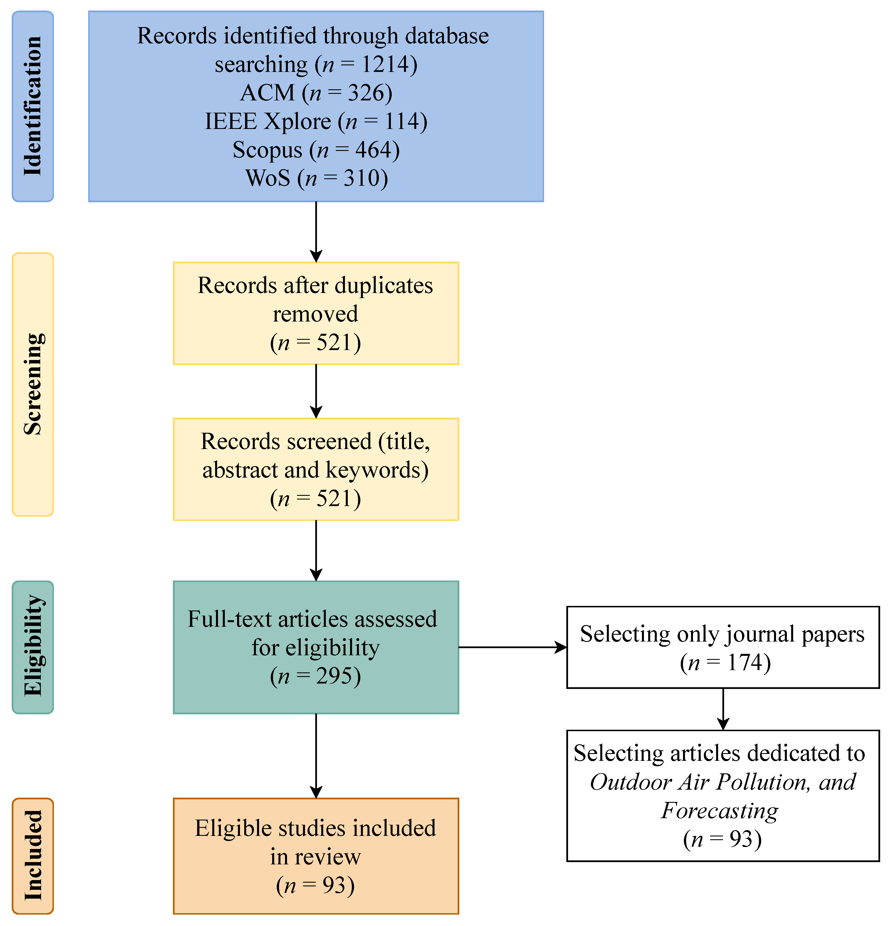
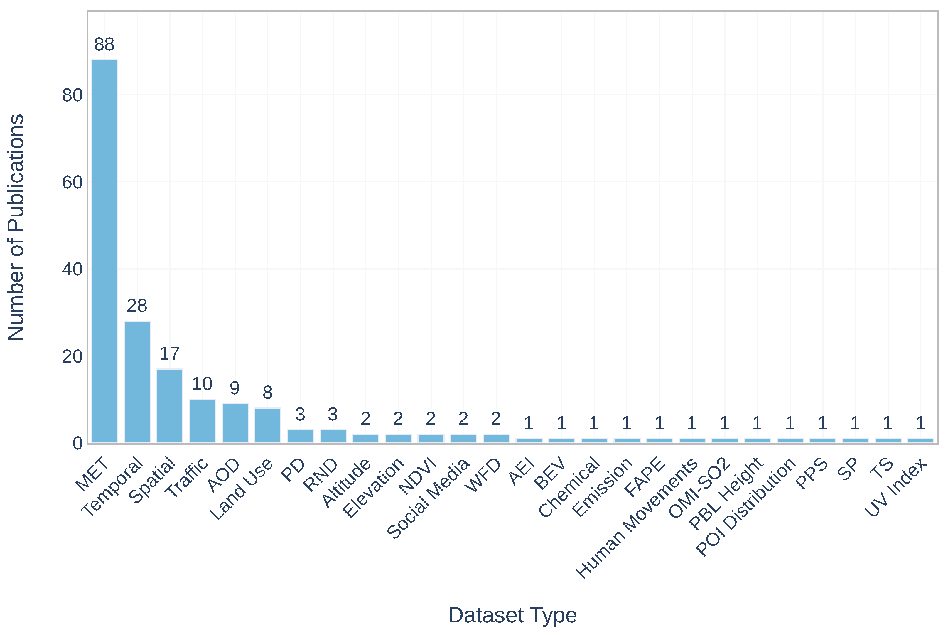


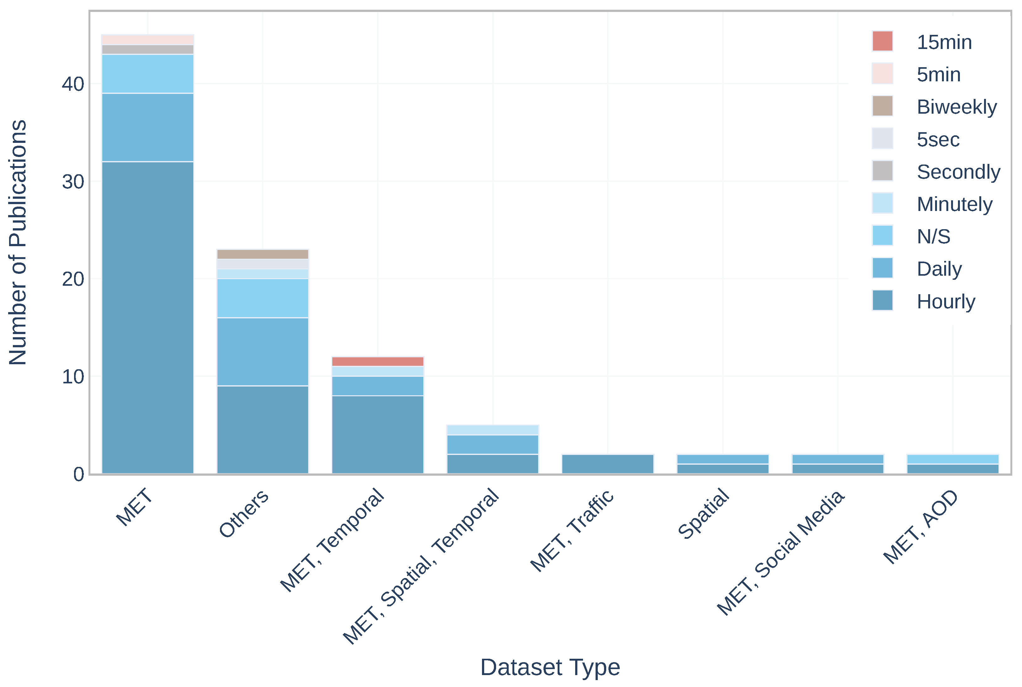
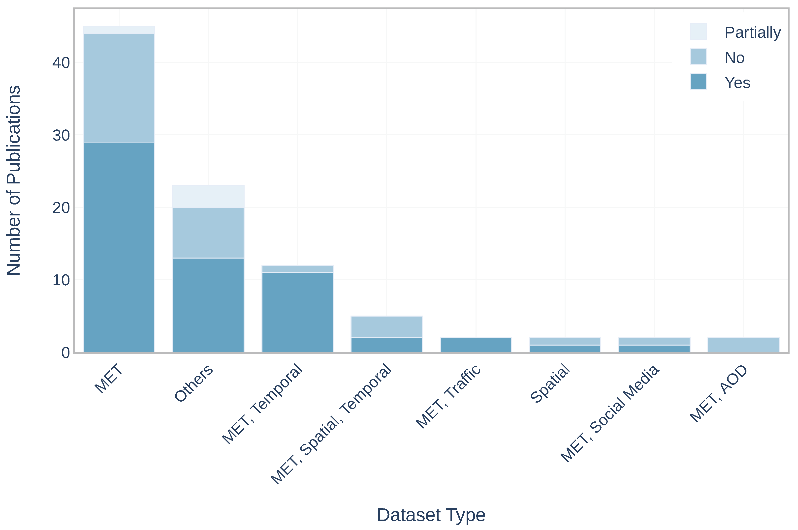
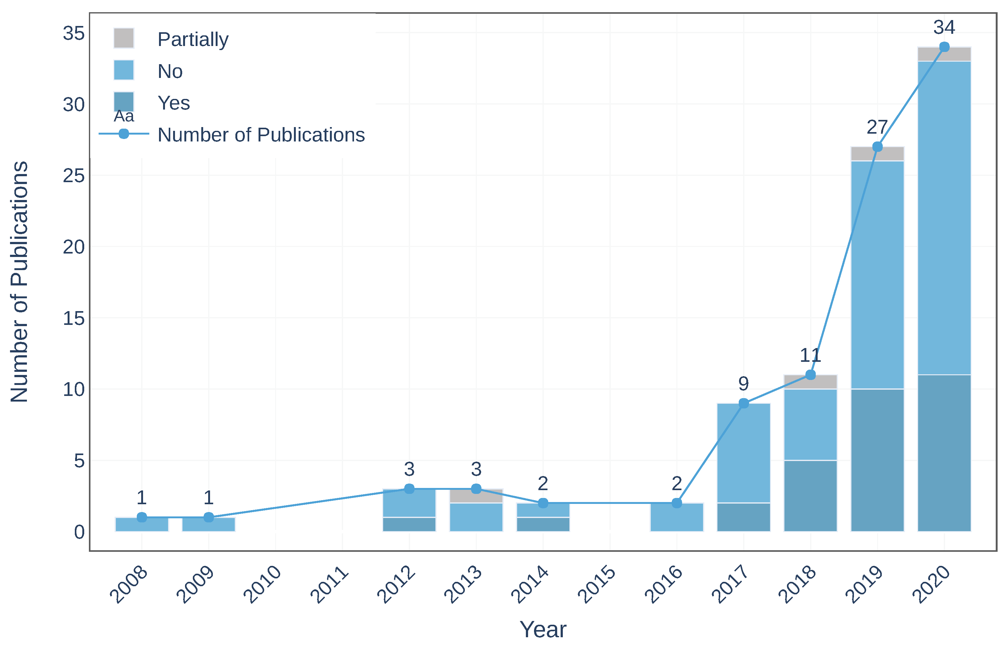
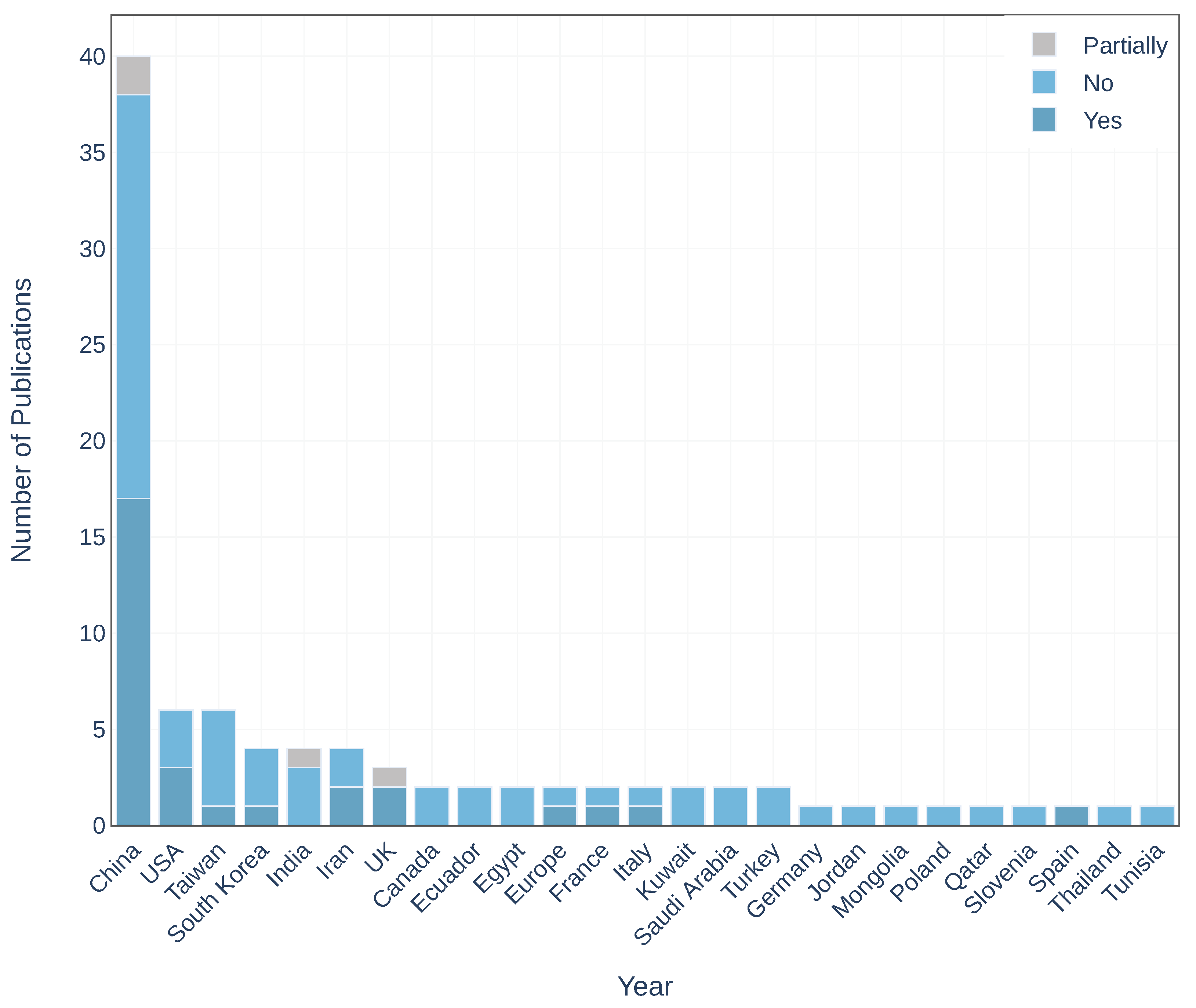
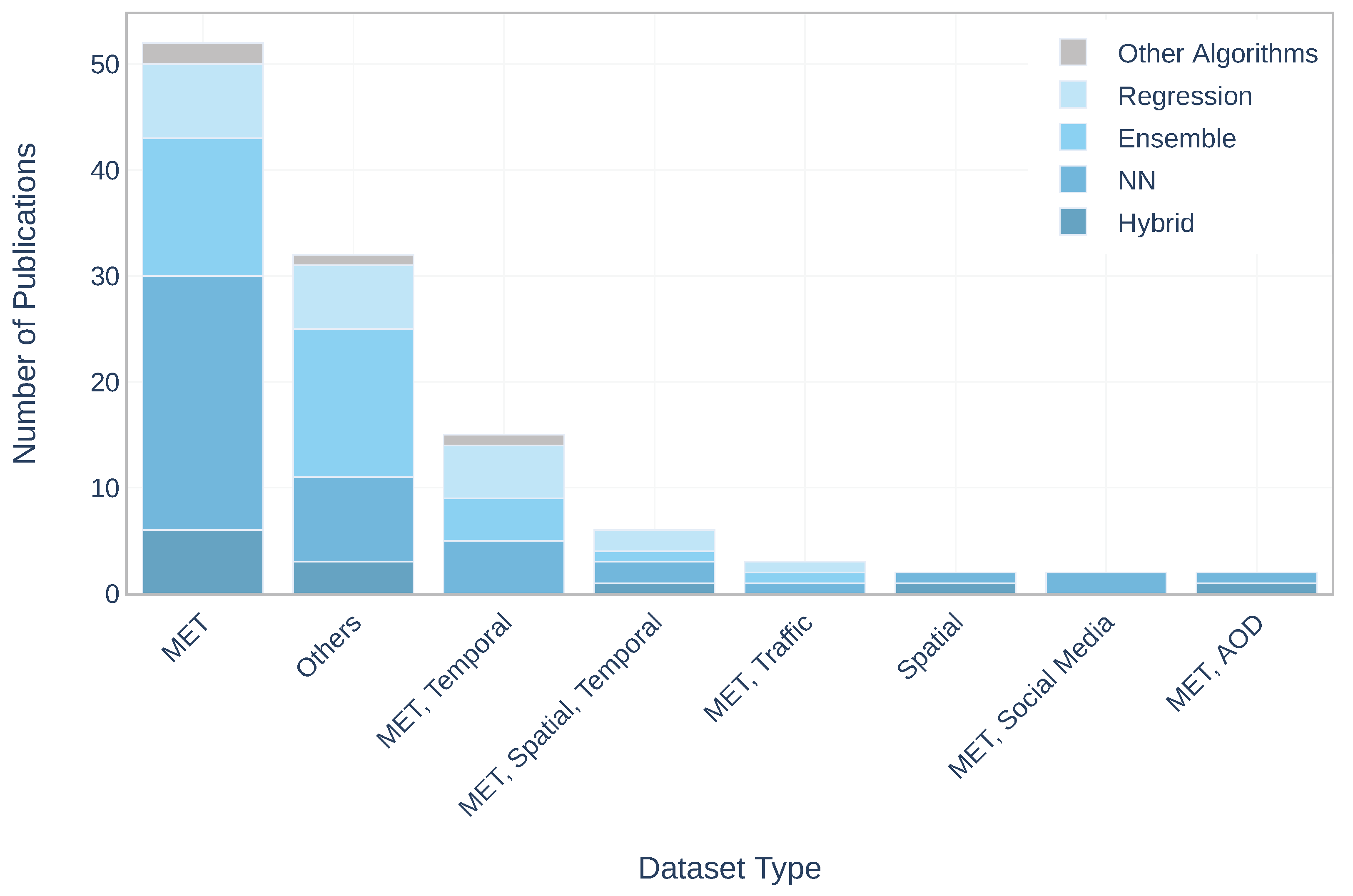
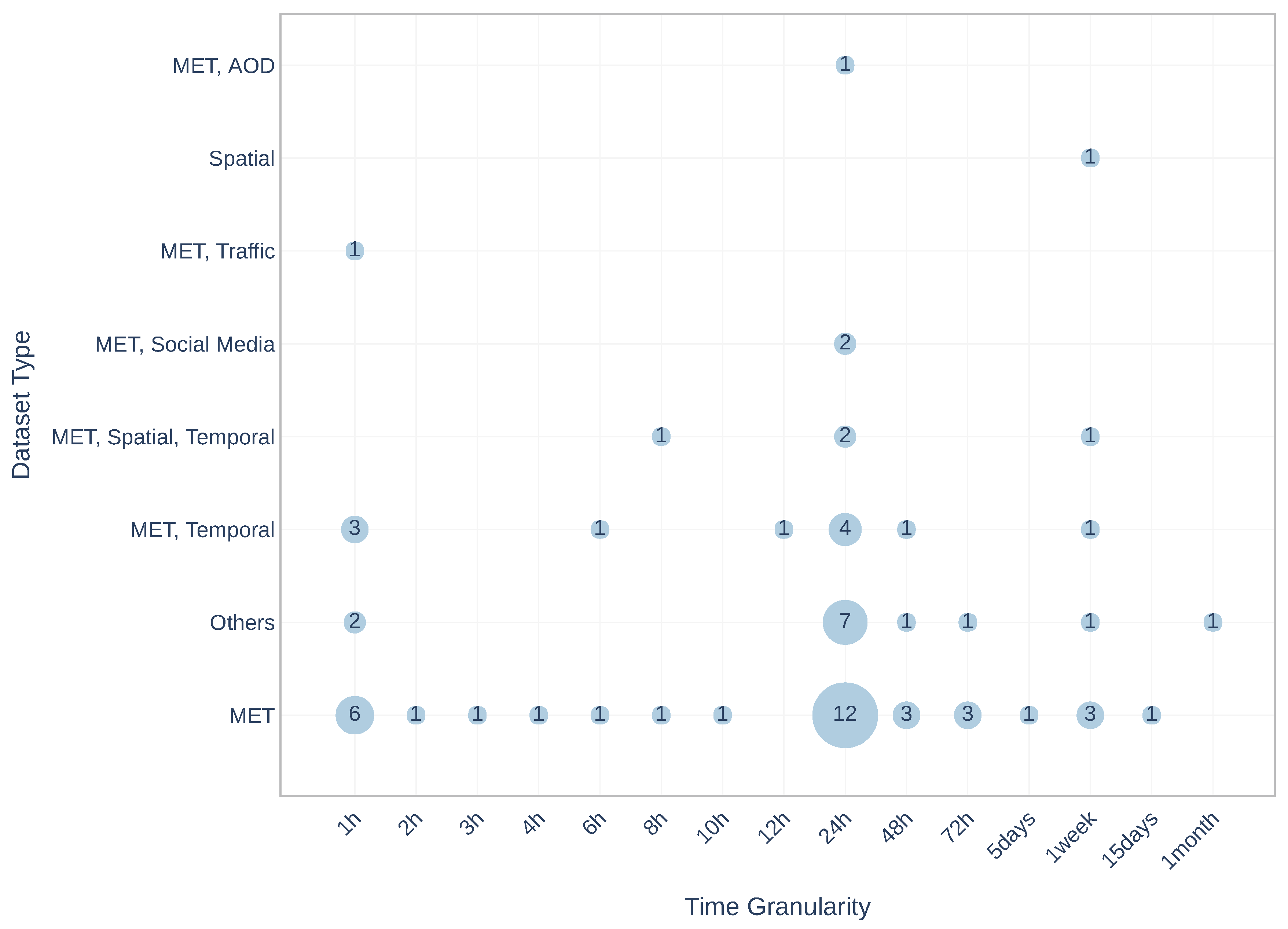
| Inclusion Criteria | Exclusion Criteria |
|---|---|
| Papers written in English | Non-English written papers |
| Publications in scientific journals | Non-reviewed papers, editorials, presentations |
| Publications until 28 September 2020 | Publications after 28 September 2020 |
| Publications focused on outdoor air pollution | Publications focused on indoor air pollution |
| Extra dataset together with air quality data | Using only air quality data |
| Analysis with implementation of ML techniques | Analysis without implementation of ML techniques |
| Models applied for forecasting purpose | Works without forecasting models |
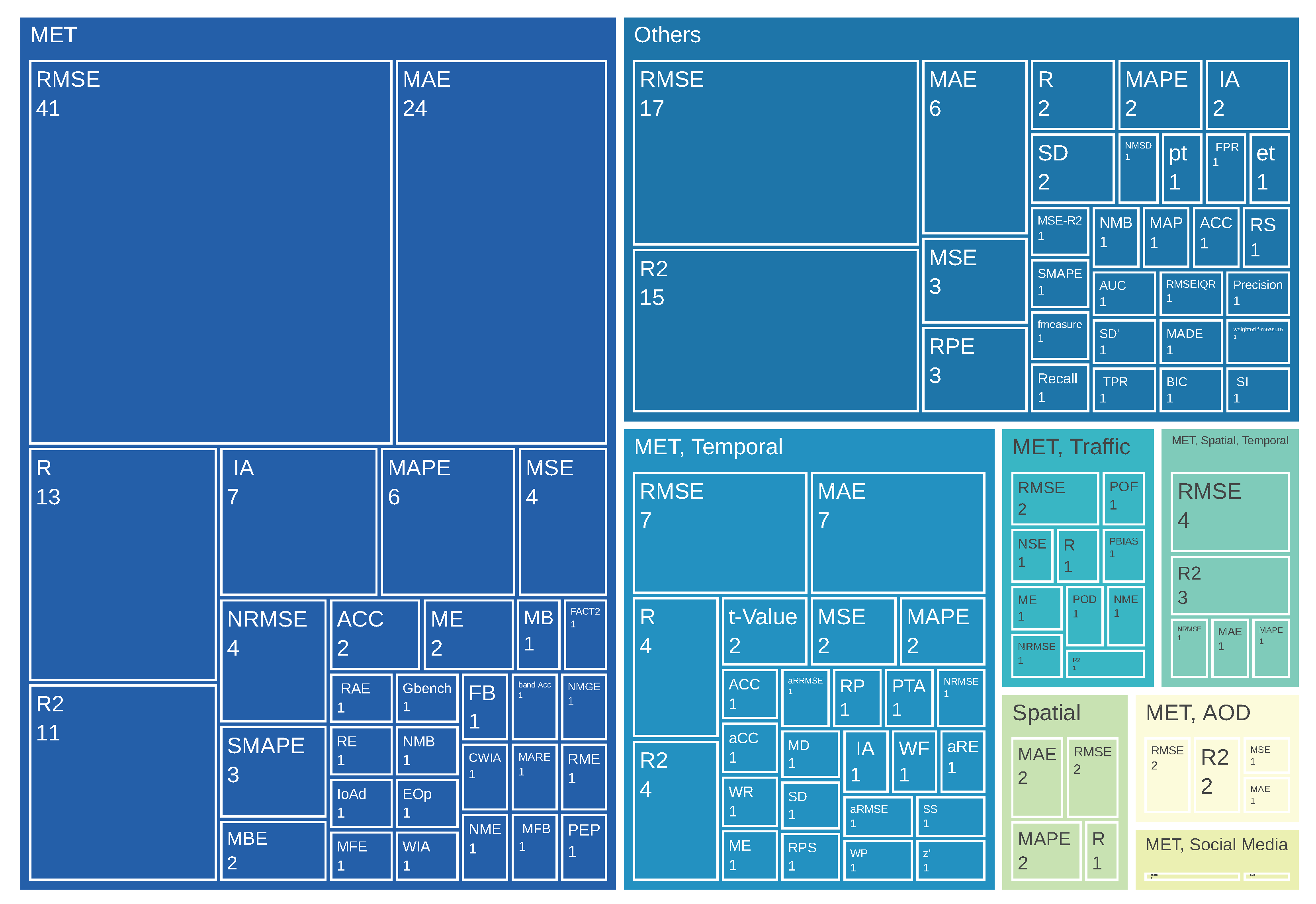
| Dataset Combinations | Publications Numbers |
|---|---|
| MET | 45 |
| MET, Temporal | 11 |
| MET, Spatial, Temporal | 5 |
| Spatial | 3 |
| MET, AOD | 2 |
| MET, Traffic | 2 |
| MET, Social Media | 2 |
| Others | 23 |
| Metrics | Equations | Description |
|---|---|---|
| RMSE | It measures the geometric difference between observed and predict data. | |
| MAE | It measures the average magnitude of the errors in a set of predictions, without considering their direction. | |
| R2 | It shows how differences in one variable can be explained by a difference in a second variable. | |
| R | It measures the strength and the direction of a linear relationship between two variables. | |
| MAPE | It measures the size of the error in percentage terms. | |
| IA | It is the ratio of the mean square error and the potential error. | |
| MSE | It measures the average squared difference between the observed and the predict values | |
| NRMSE | It is the normalised version of RMSE, which makes easier to compare different models with different scales. |
Publisher’s Note: MDPI stays neutral with regard to jurisdictional claims in published maps and institutional affiliations. |
© 2021 by the authors. Licensee MDPI, Basel, Switzerland. This article is an open access article distributed under the terms and conditions of the Creative Commons Attribution (CC BY) license (http://creativecommons.org/licenses/by/4.0/).
Share and Cite
Iskandaryan, D.; Ramos, F.; Trilles, S. Features Exploration from Datasets Vision in Air Quality Prediction Domain. Atmosphere 2021, 12, 312. https://doi.org/10.3390/atmos12030312
Iskandaryan D, Ramos F, Trilles S. Features Exploration from Datasets Vision in Air Quality Prediction Domain. Atmosphere. 2021; 12(3):312. https://doi.org/10.3390/atmos12030312
Chicago/Turabian StyleIskandaryan, Ditsuhi, Francisco Ramos, and Sergio Trilles. 2021. "Features Exploration from Datasets Vision in Air Quality Prediction Domain" Atmosphere 12, no. 3: 312. https://doi.org/10.3390/atmos12030312
APA StyleIskandaryan, D., Ramos, F., & Trilles, S. (2021). Features Exploration from Datasets Vision in Air Quality Prediction Domain. Atmosphere, 12(3), 312. https://doi.org/10.3390/atmos12030312


