
Estimating the CMIP6 Anthropogenic Aerosol Radiative Effects with the Advantage of Prescribed Aerosol Forcing


Abstract
1. Introduction
2. Methods
2.1. The GAMIL Model with MACv2-SP
2.2. Calculation Method and Updated Diagnostic Package
2.3. Experimental Design
3. Results
3.1. Annual Mean Results
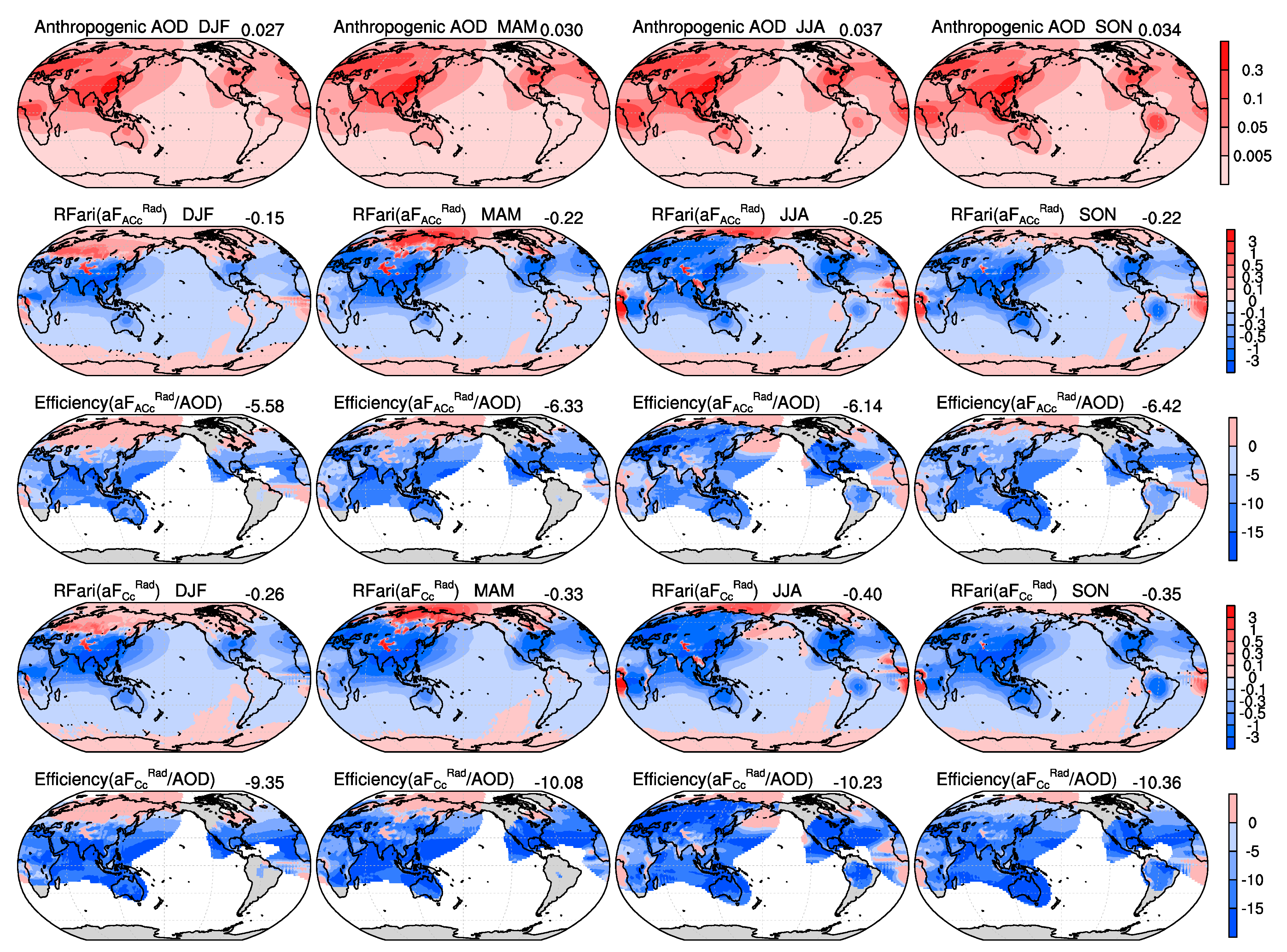
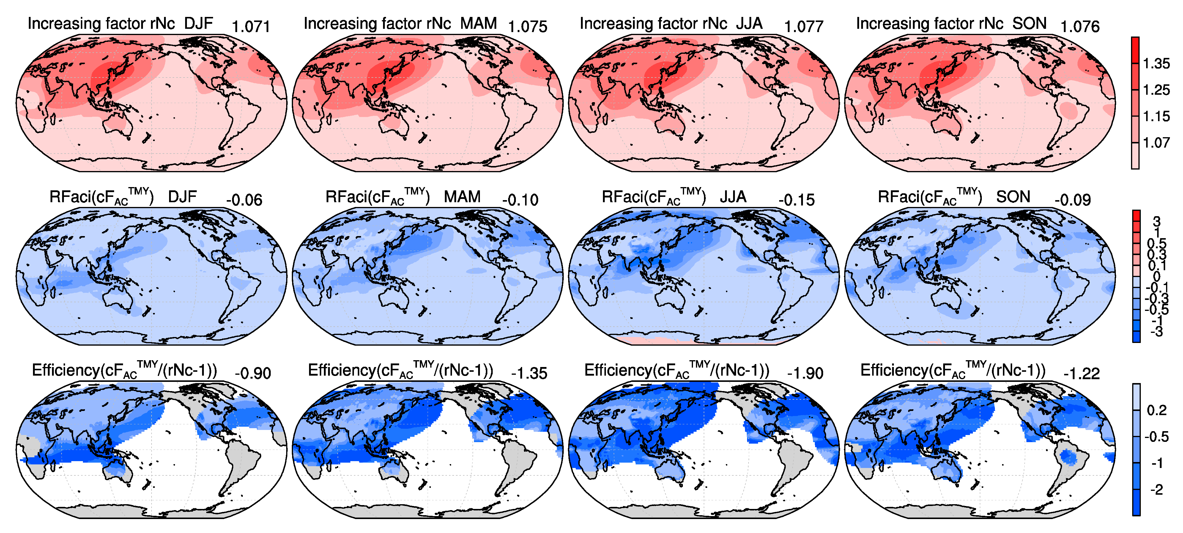
3.2. Seasonal Variability
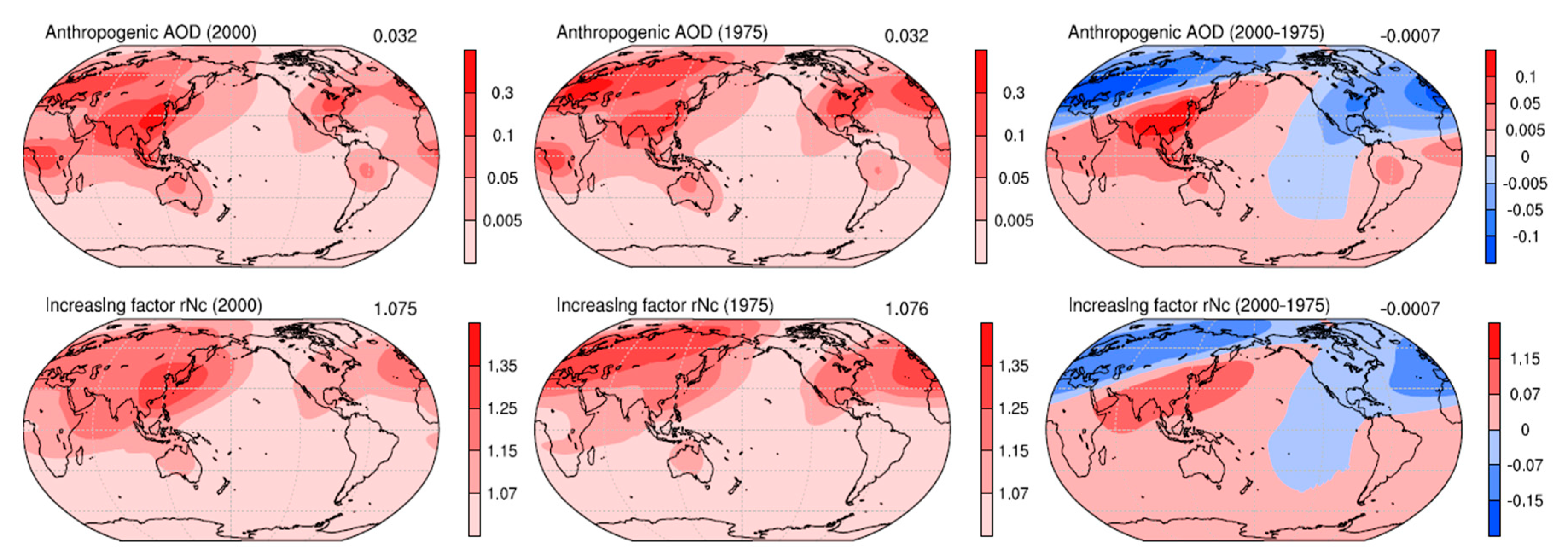
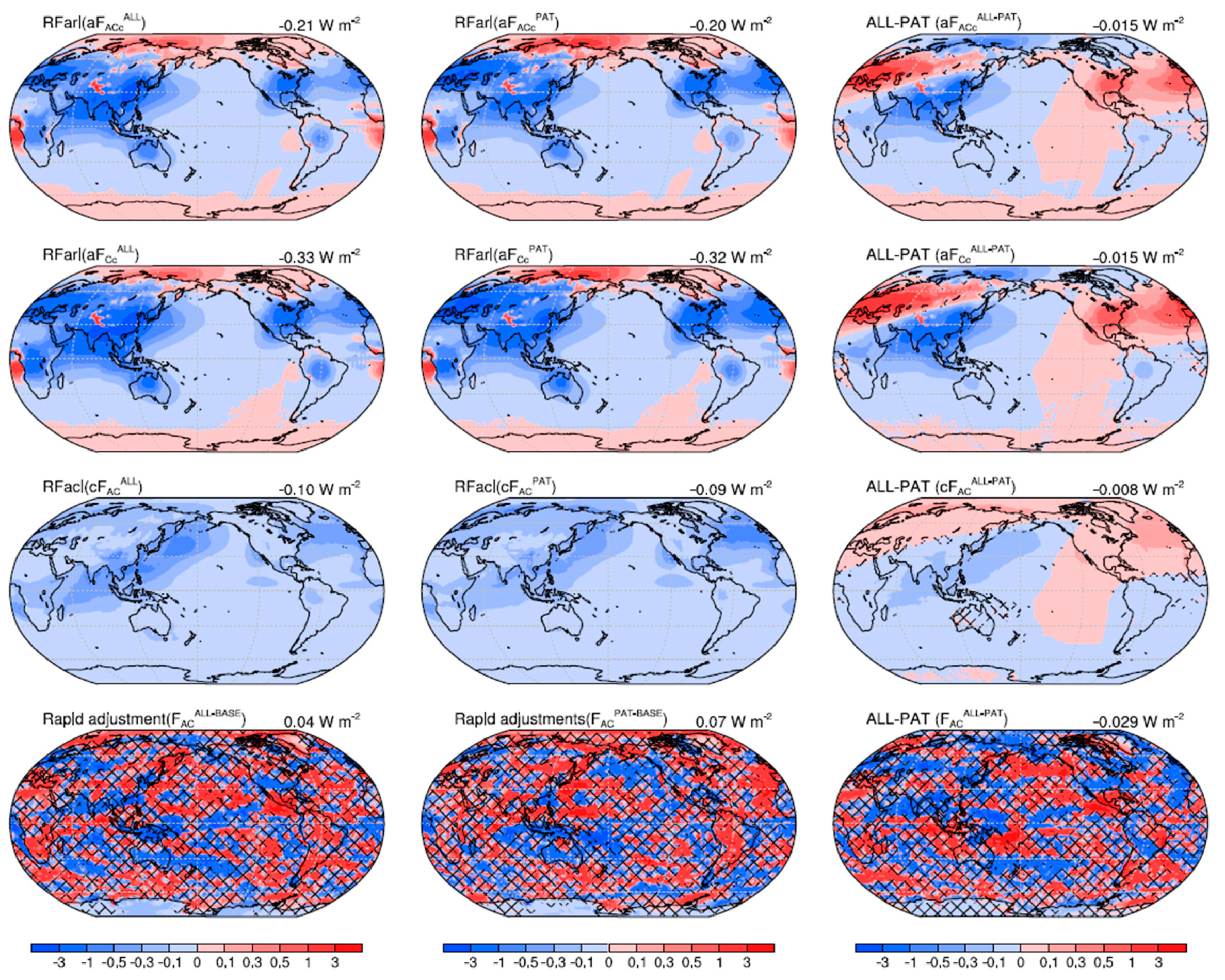
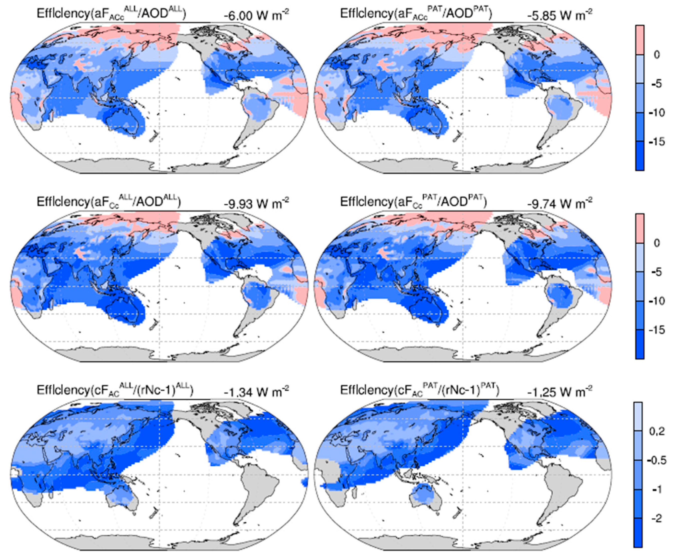
3.3. Impact of Spatial Distributions
4. Conclusions and Discussion
Author Contributions
Funding
Data Availability Statement
Acknowledgments
Conflicts of Interest
Appendix A

| BASE | RAD−BASE | ALL–TMY | TMY−BASE | ALL−RAD | ALL−BASE | PAT−BASE | |
|---|---|---|---|---|---|---|---|
| FAaCc | 237.96 | −0.22 (0.17) | −0.09 (0.15) | −0.19 (0.17) | −0.05 (0.16) | −0.27 (0.13) | −0.22 (0.15) |
| FAC | 237.96 | −0.01 (0.17) | 0.12 (0.15) | −0.09 (0.17) | 0.05 (0.16) | 0.04 (0.13) | 0.07 (0.15) |
| FA | 285.18 | 0 (0.05) | 0.01 (0.07) | −0.02 (0.07) | −0.01 (0.05) | −0.01 (0.05) | 0.03 (0.05) |
| F | 293.75 | 0 (0.06) | 0.01 (0.07) | −0.02 (0.07) | −0.01 (0.06) | −0.01 (0.05) | 0.03 (0.05) |
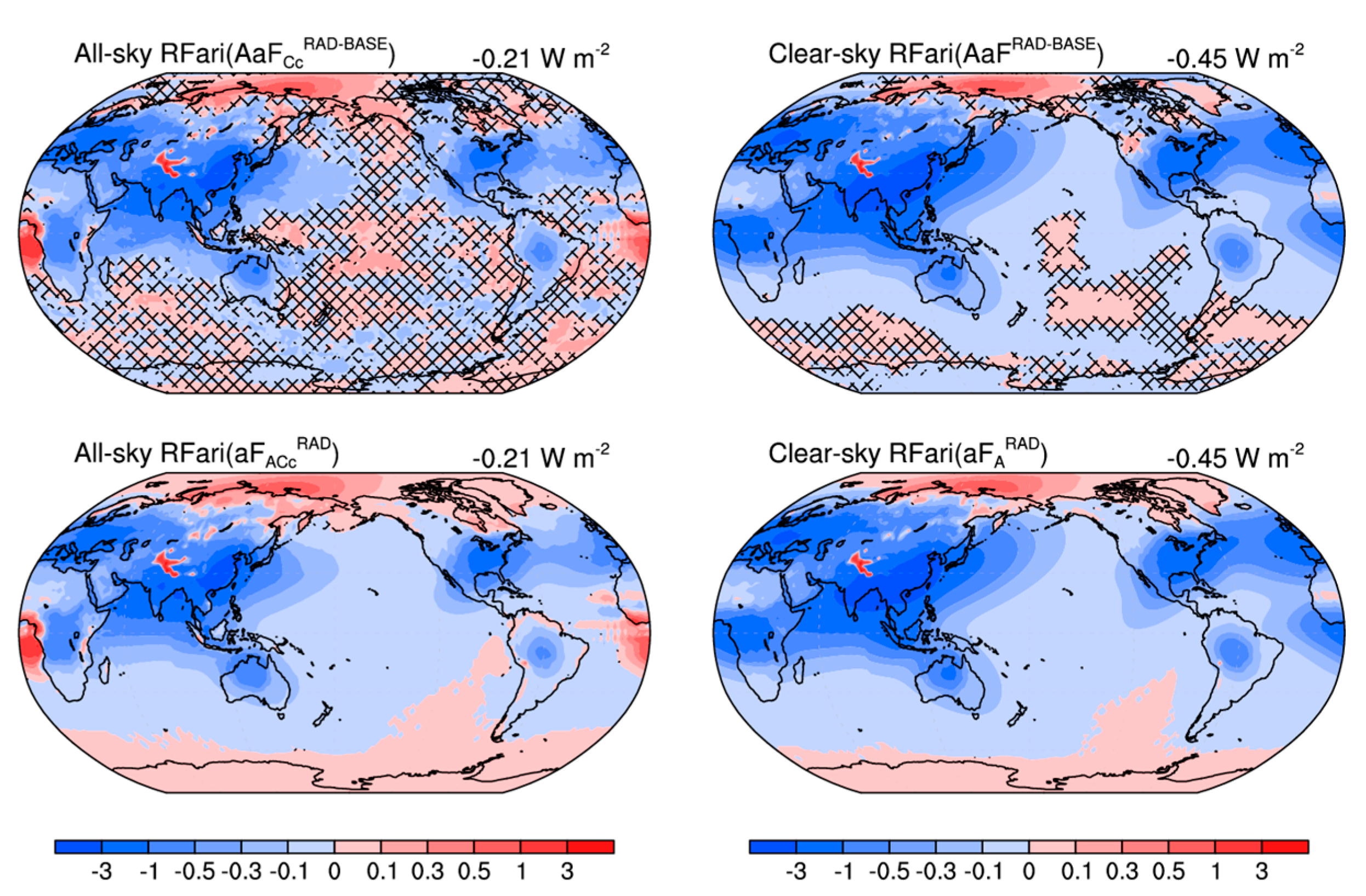
| AaFCc | −5.74 | −0.21 (0.01) | −0.22 (0.01) | 0.01 (0.01) | 0 (0.01) | −0.21 (0.01) | −0.20 (0.01) |
| AaF | −8.58 | −0.45 (0.01) | −0.45 (0.01) | 0 (0) | 0 (0) | −0.45 (0.01) | −0.43 (0.01) |
| aFACc | −0.21 (0) | −0.21(0) | 0 (0) | −0.21 (0) | −0.20 (0) | ||
| aFA | −0.45 (0) | −0.45 (0) | 0 (0) | −0.45 (0) | −0.42 (0) | ||
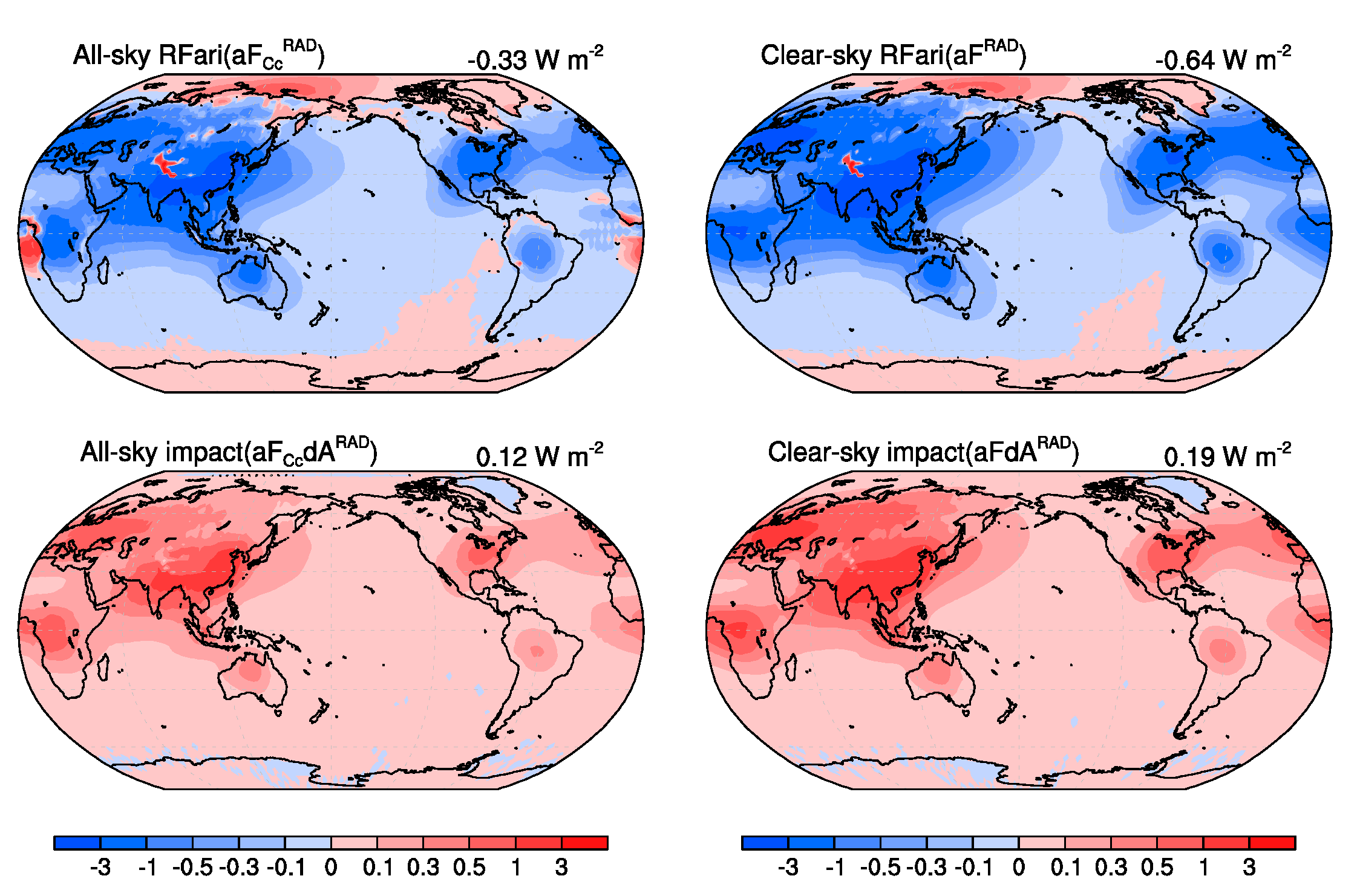
| aFCc | −0.33 (0) | −0.33 (0) | 0 (0) | −0.33 (0.01) | −0.32 (0) | ||
| aF | −0.64 (0) | −0.64 (0) | 0 (0) | −0.64 (0) | −0.61 (0) | ||
| aFAC | −0.21 (0) | −0.21 (0) | 0 (0) | −0.21(0) | −0.20 (0) | ||
| aFCcdA | 0.12 (0) | 0.12 (0) | 0 (0) | 0.12 (0) | 0.12 (0) | ||
| aFdA | 0.19 (0) | 0.19 (0) | 0 (0) | 0.19 (0) | 0.19 (0) | ||
| CcFAa | −47.22 | 0.23 (0.18) | 0.36 (0.15) | −0.17 (0.16) | −0.04 (0.17) | 0.19 (0.13) | 0.17 (0.15) |
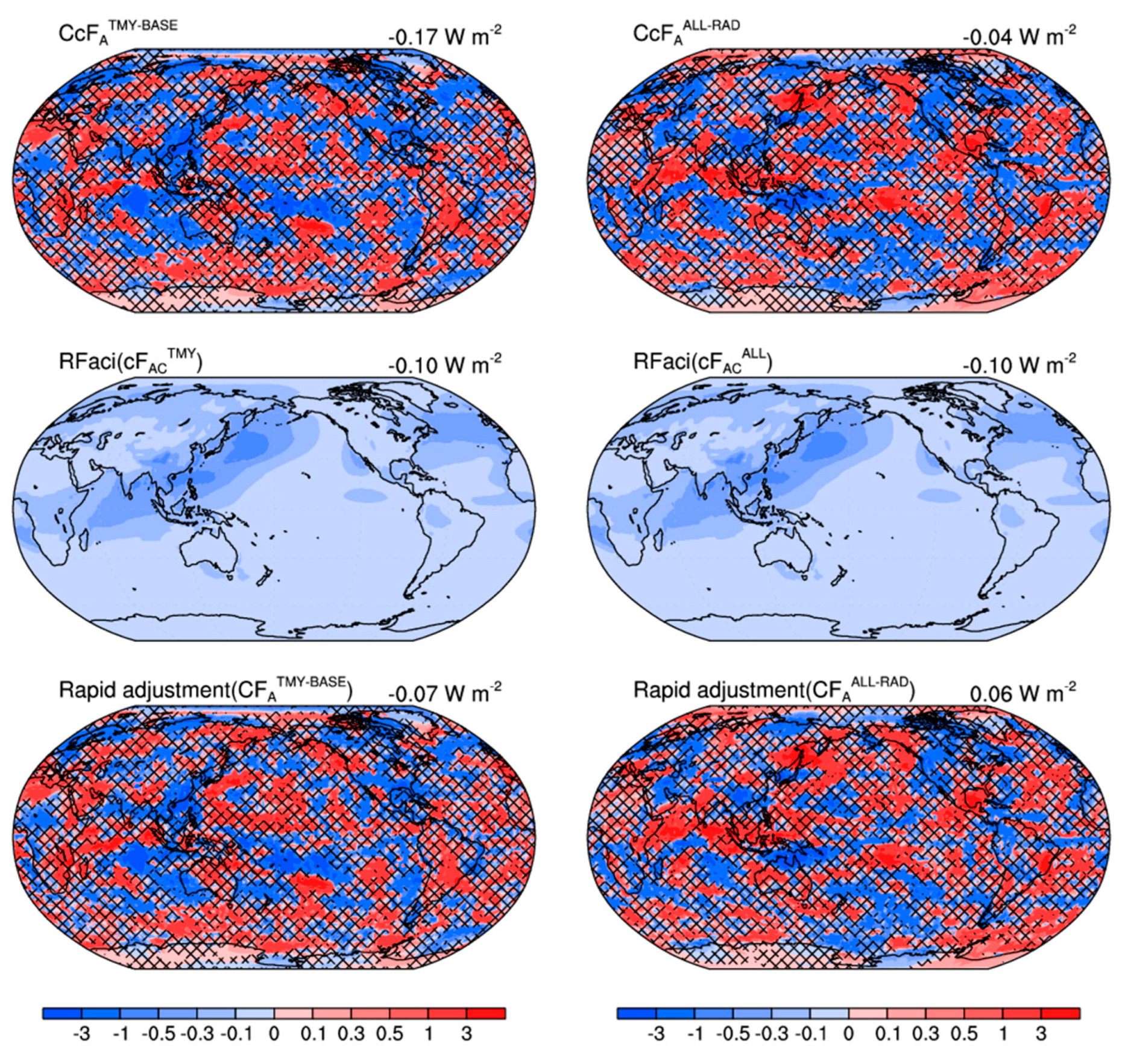
| CcF | −50.05 | −0.01 (0.19) | 0.12 (0.15) | −0.17 (0.17) | −0.04 (0.18) | −0.05 (0.14) | −0.06 (0.15) |
| CcFA | −47.22 | −0.01 (0.18) | 0.12 (0.15) | −0.17 (0.16) | −0.04 (0.17) | −0.05 (0.13) | −0.05 (0.14) |
| CFAa | −47.22 | 0.23 (0.18) | 0.35 (0.15) | −0.07 (0.16) | 0.06 (0.17) | 0.29 (0.13) | 0.27 (0.14) |
| CFA | −47.22 | −0.01 (0.18) | 0.12 (0.15) | −0.07 (0.16) | 0.06 (0.17) | 0.05 (0.13) | 0.04 (0.14) |
| cFAaC | 0 (0) | −0.10 (0) | −0.10 (0) | −0.10 (0) | −0.09 (0) | ||
| cFAC | 0 (0) | −0.10 (0) | −0.10 (0) | −0.10 (0) | −0.09 (0) |
References
- Eyring, V.; Bony, S.; Meehl, G.A.; Senior, C.A.; Stevens, B.; Stouffer, R.J.; Taylor, K.E. Overview of the Coupled Model Intercomparison Project Phase 6 (CMIP6) experimental design and organization. Geosci. Model Dev. 2016, 9, 1937–1958. [Google Scholar] [CrossRef]
- Myhre, G.; Myhre, C.E.L.; Samset, B.H.; Storelvmo, T. Aerosols and their Relation to Global Climate and Climate Sen-sitivity. Nature 2013, 4, 7. [Google Scholar]
- Stouffer, R.J.; Eyring, V.; Meehl, G.A.; Bony, S.; Senior, C.; Stevens, B.; Taylor, K.E. CMIP5 Scientific Gaps and Recommendations for CMIP6. Bull. Am. Meteorol. Soc. 2017, 98, 95–105. [Google Scholar] [CrossRef]
- Pincus, R.; Forster, P.M.; Stevens, B. The Radiative Forcing Model Intercomparison Project (RFMIP): Experimental protocol for CMIP6. Geosci. Model Dev. 2016, 9, 3447–3460. [Google Scholar] [CrossRef]
- Sanchez, K.J.; Roberts, G.C.; Calmer, R.; Nicoll, K.; Hashimshoni, E.; Rosenfeld, D.; Ovadnevaite, J.; Preissler, J.; Ceburnis, D.; O’Dowd, C.; et al. Top-down and bottom-up aerosol–cloud closure: Towards understanding sources of uncertainty in deriving cloud shortwave radiative flux. Atmos. Chem. Phys. Discuss. 2017, 17, 9797–9814. [Google Scholar] [CrossRef]
- Fiedler, S.; Stevens, B.; Mauritsen, T. On the sensitivity of anthropogenic aerosol forcing to model-internal variability and parameterizing a twomey effect. J. Adv. Model. Earth. Sy. 2017, 9, 1325–1341. [Google Scholar] [CrossRef]
- Stevens, B.; Fiedler, S.; Kinne, S.; Peters, K.; Rast, S.; Müsse, J.; Smith, S.J.; Mauritsen, T. MACv2-SP: A parameterization of anthropogenic aerosol optical properties and an associated Twomey effect for use in CMIP6. Geosci. Model Dev. 2017, 10, 433–452. [Google Scholar] [CrossRef]
- Boucher, O.; Randall, D.; Artaxo, P.; Bretherton, C.; Feingold, G.; Forster, P.; Kerminen, V.M.; Kondo, Y.; Liao, H.; Lohmann, U.; et al. Clouds and Aerosols. In Climate Change 2013: The Physical Science Basis; Cambridge University Press: Cambridge, UK, 2013. [Google Scholar]
- Ghan, S.J. Technical Note: Estimating aerosol effects on cloud radiative forcing. Atmos. Chem. Phys. Discuss. 2013, 13, 9971–9974. [Google Scholar] [CrossRef]
- Sherwood, S.C.; Bony, S.; Boucher, O.; Bretherton, C.S.; Forster, P.M.; Gregory, J.M.; Stevens, B. Adjustments in the Forcing-Feedback Framework for Understanding Climate Change. Bull. Am. Meteorol. Soc. 2015, 96, 217–228. [Google Scholar] [CrossRef]
- Bellouin, N.; Quaas, J.; Gryspeerdt, E.; Kinne, S.; Stier, P.; Watson-Parris, D.; Boucher, O.; Carslaw, K.S.; Christensen, M.; Daniau, A.; et al. Bounding Global Aerosol Radiative Forcing of Climate Change. Rev. Geophys. 2020, 58, 1–69. [Google Scholar] [CrossRef] [PubMed]
- Boucher, O.; Lohmann, U. The sulfate-CCN-cloud albedo effect: A sensitivity study with two general circulation models. Tellus 1995, 47, 281–300. [Google Scholar] [CrossRef]
- Fiedler, S.; Kinne, S.; Huang, W.T.K.; Räisänen, P.; O’Donnell, D.; Bellouin, N.; Stier, P.; Merikanto, J.; Van Noije, T.; Makkonen, R.; et al. Anthropogenic aerosol forcing–insights from multiple estimates from aerosol-climate models with reduced complexity. Atmos. Chem. Phys. Discuss. 2019, 19, 6821–6841. [Google Scholar] [CrossRef]
- Shi, X.; Zhang, W.; Liu, J. Comparison of Anthropogenic Aerosol Climate Effects among Three Climate Models with Reduced Complexity. Atmosphere 2019, 10, 456. [Google Scholar] [CrossRef]
- Smith, S.J.; Van Aardenne, J.; Klimont, Z.; Andres, R.J.; Volke, A.; Arias, S.D. Anthropogenic sulfur dioxide emissions: 1850–2005. Atmos. Chem. Phys. Discuss. 2011, 11, 1101–1116. [Google Scholar] [CrossRef]
- Shindell, D.T.; Lamarque, J.F.; Schulz, M.; Flanner, M.; Yoon, J.H. Radiative forcing in the ACCMIP historical and future climate simulations. Atmos. Chem. Phys. 2013, 13, 2939–2974. [Google Scholar] [CrossRef]
- Li, L.; Dong, L.; Xie, J.; Tang, Y.; Xie, F.; Guo, Z.; Liu, H.; Feng, T.; Wang, L.; Pu, Y.; et al. The GAMIL3: Model Description and Evaluation. J. Geophys. Res. Atmos. 2020, 125, 125. [Google Scholar] [CrossRef]
- Twomey, S. The Influence of Pollution on the Shortwave Albedo of Clouds. J. Atmos. Sci. 1977, 34, 1149–1152. [Google Scholar] [CrossRef]
- Yang, J.; Wang, B.; Guo, Y.; Wan, H.; Ji, Z. Comparison between GAMIL, and CAM2 on interannual variability simulation. Adv. Atmos. Sci. 2007, 24, 82–88. [Google Scholar] [CrossRef]
- Li, L.; Wang, Y.; Wang, B.; Zhou, T. Sensitivity of the Grid-point Atmospheric Model of IAP LASG (GAMIL1.1.0) climate simulations to cloud droplet effective radius and liquid water path. Adv. Atmos. Sci. 2008, 25, 529–540. [Google Scholar] [CrossRef]
- Zhang, K.; Wan, H.; Wang, B.; Zhang, M. Consistency problem with tracer advection in the Atmospheric Model GAMIL. Adv. Atmos. Sci. 2008, 25, 306–318. [Google Scholar] [CrossRef]
- Li, L.; Lin, P.; Yu, Y.; Wang, B.; Zhou, T.; Liu, L.; Liu, J.; Bao, Q.; Xu, S.; Huang, W.; et al. The flexible global ocean-atmosphere-land system model, Grid-point Version 2: FGOALS-g2. Adv. Atmos. Sci. 2013, 30, 543–560. [Google Scholar] [CrossRef]
- Shi, X.; Wang, B.; Liu, X.; Wang, M. Two-moment bulk stratiform cloud microphysics in the grid-point atmospheric model of IAP LASG (GAMIL). Adv. Atmos. Sci. 2013, 30, 868–883. [Google Scholar] [CrossRef]
- Briegleb, B.P. Delta-Eddington approximation for solar radiation in the NCAR community climate model. J. Geophys. Res. Space Phys. 1992, 97, 7603. [Google Scholar] [CrossRef]
- Collins, W.D. A global signature of enhanced shortwave absorption by clouds. J. Geophys. Res. Space Phys. 1998, 103, 31669–31679. [Google Scholar] [CrossRef]
- Kinne, S. Aerosol radiative effects with MACv2. Atmos. Chem. Phys. Discuss. 2019, 19, 10919–10959. [Google Scholar] [CrossRef]
- Myhre, G.; Samset, B.H.; Schulz, M.; Balkanski, Y.; Bauer, S.; Berntsen, T.K.; Bian, H.; Bellouin, N.; Chin, M.; Diehl, T.; et al. Radiative forcing of the direct aerosol effect from AeroCom Phase II simulations. Atmos. Chem. Phys. Discuss. 2013, 13, 1853–1877. [Google Scholar] [CrossRef]
- Carslaw, K.S.; Gordon, H.; Hamilton, D.S.; Johnson, J.S.; Regayre, L.A.; Yoshioka, M.; Pringle, K.J. Aerosols in the Pre-industrial Atmosphere. Curr. Clim. Chang. Rep. 2017, 3, 1–15. [Google Scholar] [CrossRef] [PubMed]


| Names (W m–2) | Natural Aerosol Optical Properties (“A”) | Anthropogenic Aerosol Optical Properties (“a”) | Cloud Optical Properties with the Twomey Effect (“Cc”) | Background Cloud Optical Properties (“C”) |
|---|---|---|---|---|
| FAaCc | Х | Х | Х | |
| FAa | Х | Х | ||
| FACc | Х | Х | ||
| FA | Х | |||
| FaCc | Х | Х | ||
| Fa | Х | |||
| FCc | Х | |||
| F | ||||
| FAaC | Х | Х | Х | |
| FAC | Х | Х |
| Names | Description | Equation |
|---|---|---|
| AaFCc | Shortwave total aerosol RF | AaFCc = FAaCc − FC |
| AaF | Clear-sky AaFCc | AaF = FAa − F |
| aFACc | Shortwave anthropogenic aerosol RF | aFACc = FAaCc − FACc. |
| aFA | Clear-sky aFACc | aFA = FAa − FA |
| aFCc | aFACc without natural aerosol radiative effect | aFCc = FaCc − FCc. |
| aF | Clear-sky aFCc | aF = Fa − F |
| aFAC | aFACc excluding Twomey effect | aFAC = FAaC − FAC. |
| aFCcdA | Impact of natural aerosol on calculating aFCc | aFCcdA = aFACc − aFCc |
| aFdA | Clear-sky aFCcdA | aFdA = aFA − aF |
| CcFAa | Shortwave cloud forcing | CcFAa = FAaCc − FAa |
| CcF | CcFAa without total aerosol radiative effect | CcF = FCc − F |
| CcFA | CcFAa without anthropogenic aerosol radiative effect | CcFA = FACc − FA |
| CFAa | CcFAa excluding Twomey effect | CFAa = FAaC − FAa |
| CFA | CcFA excluding Twomey effect | CFA = FAC − FA |
| cFAaC | Twomey effect on cloud forcing | cFAaC = CcFAa − CFAa = FAaCc − FAaC |
| cFAC | cFAaC without anthropogenic aerosol radiative effect | cFAC = CcFA − CFA = FACc − FAC |
| Names | Anthropogenic Aerosol Radiative Forcing (“a”) | Anthropogenic Aerosol Twomey Effect (“c”) |
|---|---|---|
| BASE | None | None |
| RAD | Year 2000 | None |
| TMY | None | Year 2000 |
| ALL | Year 2000 | Year 2000 |
| PAT | Year 1975 | Year 1975 |
Publisher’s Note: MDPI stays neutral with regard to jurisdictional claims in published maps and institutional affiliations. |
© 2021 by the authors. Licensee MDPI, Basel, Switzerland. This article is an open access article distributed under the terms and conditions of the Creative Commons Attribution (CC BY) license (http://creativecommons.org/licenses/by/4.0/).
Share and Cite
Shi, X.; Li, C.; Li, L.; Zhang, W.; Liu, J. Estimating the CMIP6 Anthropogenic Aerosol Radiative Effects with the Advantage of Prescribed Aerosol Forcing. Atmosphere 2021, 12, 406. https://doi.org/10.3390/atmos12030406
Shi X, Li C, Li L, Zhang W, Liu J. Estimating the CMIP6 Anthropogenic Aerosol Radiative Effects with the Advantage of Prescribed Aerosol Forcing. Atmosphere. 2021; 12(3):406. https://doi.org/10.3390/atmos12030406
Chicago/Turabian StyleShi, Xiangjun, Chunhan Li, Lijuan Li, Wentao Zhang, and Jiaojiao Liu. 2021. "Estimating the CMIP6 Anthropogenic Aerosol Radiative Effects with the Advantage of Prescribed Aerosol Forcing" Atmosphere 12, no. 3: 406. https://doi.org/10.3390/atmos12030406
APA StyleShi, X., Li, C., Li, L., Zhang, W., & Liu, J. (2021). Estimating the CMIP6 Anthropogenic Aerosol Radiative Effects with the Advantage of Prescribed Aerosol Forcing. Atmosphere, 12(3), 406. https://doi.org/10.3390/atmos12030406