Article

Investigation of Aerosol Direct Effect over China under El Niño and Its Spatial Distribution Using WRF-Chem

1
School of Atmospheric Sciences, and Guangdong Province Key Laboratory for Climate Change and Natural Disaster Studies, Sun Yat-sen University, Guangzhou 510275, China
2
Southern Marine Science and Engineering Guangdong Laboratory, Zhuhai 519000, China
3
School of Geography and Tourism, Huizhou University, Huizhou 516000, China
*
Authors to whom correspondence should be addressed.
Atmosphere 2021, 12(1), 58; https://doi.org/10.3390/atmos12010058
Submission received: 26 November 2020 / Revised: 24 December 2020 / Accepted: 25 December 2020 / Published: 31 December 2020

Abstract

:
With rapid economic development and urbanization, the air pollution problem over China has drawn great attention. To explore the aerosol direct effect (ADE) over China, two simulations were conducted using WRF-Chem V3.5.1 in the summer of 2015. One was a control run (CTL) including aerosol effect and related physical and chemical processes, and the other one was a sensitivity simulation (SEN), the same as CTL except that aerosol-radiation interactions were turned off. The differences between two tests were analyzed, in particular over regions in South China (SC) and East China (EC). Results showed the following. (1) The large-scale circulation showed a strong El Niño signal, associated with cooling and wet anomalies over EC, while warming and dry anomalies over EC. (2) Due to ADE, there was a significant decrease in precipitation and an increase in AOD over SC and EC, albeit with different mechanisms. (3) In SC, ADE cooled the region reinforcing the El Niño impact and suppressing water vapor fluxes, which led to a more stable atmosphere and weakened water cycle. In EC, ADE caused vertical circulation anomalies opposing the El Niño impact. (4) ADE showed obvious land-sea difference in precipitation and shortwave radiation.

1. Introduction

Aerosols play an important role in climate change characterized by influencing the atmosphere directly and indirectly. The aerosol direct effect (ADE) refers to cooling at the surface and warming in the atmosphere via absorbing and scattering solar radiation [1,2,3]. The aerosol indirect effect is mainly by changing the microphysical processes in which aerosols serve to act as cloud condensation nuclei (CCN) or ice nuclei (CN) [4,5,6].
With increasing aerosol emission, the air pollution problems over China have drawn great attention. There are plenty of investigations on the aerosol influences on climate over China. For example, Huang et al. [7] conducted simulations to explore the aerosol direct effect (ADE) on climate over China and found that aerosols significantly contributed to warming in the atmosphere. Li et al. [8] investigated the aerosol effect on precipitation over the Pearl River Delta region which has large aerosol loading due to rapid urbanization. It is indicated that ADE tended to enhance the generation of rainwater while the aerosol indirect effect tended to weaken precipitation. To provide a valuable perspective on emission control policies, Zhou et al. [9] investigated the relationship between PM2.5 variability and aerosol-radiation interactions. The study pointed out that emission control was much more effective under heavy polluted conditions due to aerosol-radiation interactions.
As one of the most important drivers in the climate over East Asia, ENSO(El Niño–Southern Oscillation) has certain influence on aerosol-meteorology interactions. In Abish and Mohanakumar’s study [10], it was implied that during La Nina, aerosol loading was suppressed due to a weaker zonal circulation. Chang et al. [11] showed that El Niño events were in favor of exaggerating the pollution in winter over eastern China. Kim et al. [12] suggested that ADE can drastically modulate the ENSO impact especially over the Asia monsoon area as a response to climate change. Moreover, Bellouin et al. [13] indicated that with the decreasing trend of aerosol emission atmospheric warming due to ADE might be weakened. Although plenty of research has demonstrated the important role of ADE on the regional climate over China, few studies describe the spatial distribution of ADE and the underlying mechanism, particularly under the background of ENSO. The spatial heterogeneity of ADE can provide beneficial perspective for making effective pollution control policies. Therefore, a strong El Niño event was selected here to explore ADE over China during the summer of 2015.
In this paper, the descriptions of datasets, methods and experimental design are first presented in Section 2. Main results are presented in Section 3. In Section 3.1, the simulation results are comprehensively evaluated. In Section 3.2, a composite analysis is implemented to describe the spatial characteristics of the meteorological anomalies due to ENSO. Moreover, a variation analysis is conducted to indicate the unique anomalies in the summer 2015. After that, the differences between control (CTL) and sensitivity simulation (SEN) tests are presented to demonstrate ADE over China and the associated mechanism. Finally, the conclusion and discussion follow in Section 4.

2. Data and Methodology

2.1. Model Settings

Two experiments were conducted using a WRF(Weather Research and Forecasting) model version 3.5.1, coupled with a chemistry module (WRF-Chem V3.5.1; [14,15]). One was a control test (CTL), and the other one a sensitivity test (SEN). The simulated domain (Figure 1) covered the region, 60° W–150° E, 5° S–45° N, consisting of 180 × 290 grid cells, and no nesting was applied. The horizontal resolution was 30 km × 30 km along with 42 layers vertically. The physical and chemical schemes selected for the simulation were the Yonsei University planetary boundary layer scheme [16], the Kain–Fritsch cumulus parameterization scheme [17], and the longwave and shortwave radiation scheme of the Rapid Radiative Transfer Model for general circulation models [18] (RRTMG). The gas-phase chemistry model was based on the Regional Acid Deposition Model version 2 [19], while the Modal Aerosol Dynamics Model for Europe/Secondary Organic Aerosol Model [20,21] was chosen as the driver for aerosols [14]. As microphysical processes are critical for aerosol indirect effect, a double-moment scheme, the Morrison aerosol microphysics scheme [22,23] was applied. With the Kain-Fritsch cumulus scheme, there is no feedback from the parameterized convection to the atmospheric radiation and the photolysis schemes [24]. In previous studies on simulating the aerosol effect over China [25,26,27,28,29], the selected schemes were widely adopted, and their capabilities were sufficiently demonstrated. The simulated time period covered from 0000 UTC on 26 May to 0000 UTC on 31 August 2020, with the first five days as a spin-up time. The analysis was mainly focused on the time period from June to August (JJA). Sea surface temperature (SST), sea ice, vegetation fraction and albedo were updated every 6 h (sst_update = 1). Upper-air nudging was turned on to reduce the deviation between simulation and observation. Nudging was applied to the horizontal wind and temperature with a coefficient of 0.0003 s−1 and a frequency of 60 s. The model settings are summarized in Table 1.
In the SEN test, the model settings were the same as in CTL test. To exclude the aerosol radiation impact, the aerosol direct feedback was turned off. The experimental design is presented in Table 2.

2.2. Datasets and Methods

The National Centers for Environmental Prediction (NCEP) Final Operational Global Analysis data (https://rda.ucar.edu/datasets/ds083.2/) was used as the initial and boundary conditions of the simulation. The “Reanalysis of the Tropospheric chemical composition over the past 40 yr” (RETRO, http://retro.enes.org) was used for anthropogenic emissions.
To evaluate the control simulation results, comparison was made with ERA5, fifth generation of ECMWF atmospheric reanalysis dataset [30] on fundamental metrological variables such as temperature, geopotential height, wind, precipitation and specific humidity. The ERA5 dataset is consistent with the input dataset used for simulation, NCEP, in observation and data assimilation methods. It has a spatial resolution of 0.25° × 0.25°. A 3-hourly reanalysis dataset is applied for model evaluation in Section 3.1 while the monthly mean reanalysis dataset is used for composite analysis in Section 3.2. The evaluation was based on widely used statistical methods, abnormal correlation coefficient (ACC) and normalized root mean square error (NRMSE) [31]. The significance mentioned in the following text is calculated according to the Student’s t-test. The maximum value of ACC is 1.0. The simulation performance was considered robust when ACC reached 0.6 [32]. The calculation of ACC and NRMSE are as follows:
A C C = i N ( y i s y i s ¯ ) ( y i o y i o ¯ ) N 1 N i = 1 N ( y i s y i s ¯ ) 2 1 N i = 1 N ( y i o y i o ¯ ) 2
N R M S E = 1 N i = 1 N ( y i s y i o ) 2 1 N i = 1 N y i o
where y i s and y i o represent the simulation value and reanalysis value on grid cell i , respectively. y i s ¯ and y i o ¯ represent the mean values from simulation and reanalysis data on grid cell i , respectively. While calculating ACC, N is the total number of effective times on every grid, which results in a spatial distribution of ACC. While calculating NRMSE, N is the total grid number spatially.
The classification of El Niño years and La Nina years were based on the average multivariate ENSO Index from June to August [33] (MEI). From 1979–2015, the seven highest indexes were selected as El Niño years (1982, 1983, 1987, 1993, 1997, 2009, and 2015), and the seven lowest were selected as La Nina years (1988, 1989, 1999, 2007, 2010, 2011, and 2013).

3. Results

3.1. Model Evaluation

The simulation performance was evaluated based on the comparison between CTL test result and ERA5 datasets on temperature at 2 m, specific humidity at 700 hPa, precipitation rate, geopotential height and wind fields at 850 hPa and 500 hPa. The pattern correlations and NRMSEs of the JJA average fields between simulation and reanalysis data were calculated and are illustrated in Table 3. All the pattern correlations passed the significant test at a level of 99% and were higher than 0.7, indicating good performance of the simulation in reproducing the distributions of these meteorological variables, especially specific humidity, temperature and wind. The NRMSEs were generally small, with those of specific humidity, temperature and geopotential height less than 0.001, while those of precipitation rate and wind were relatively larger.
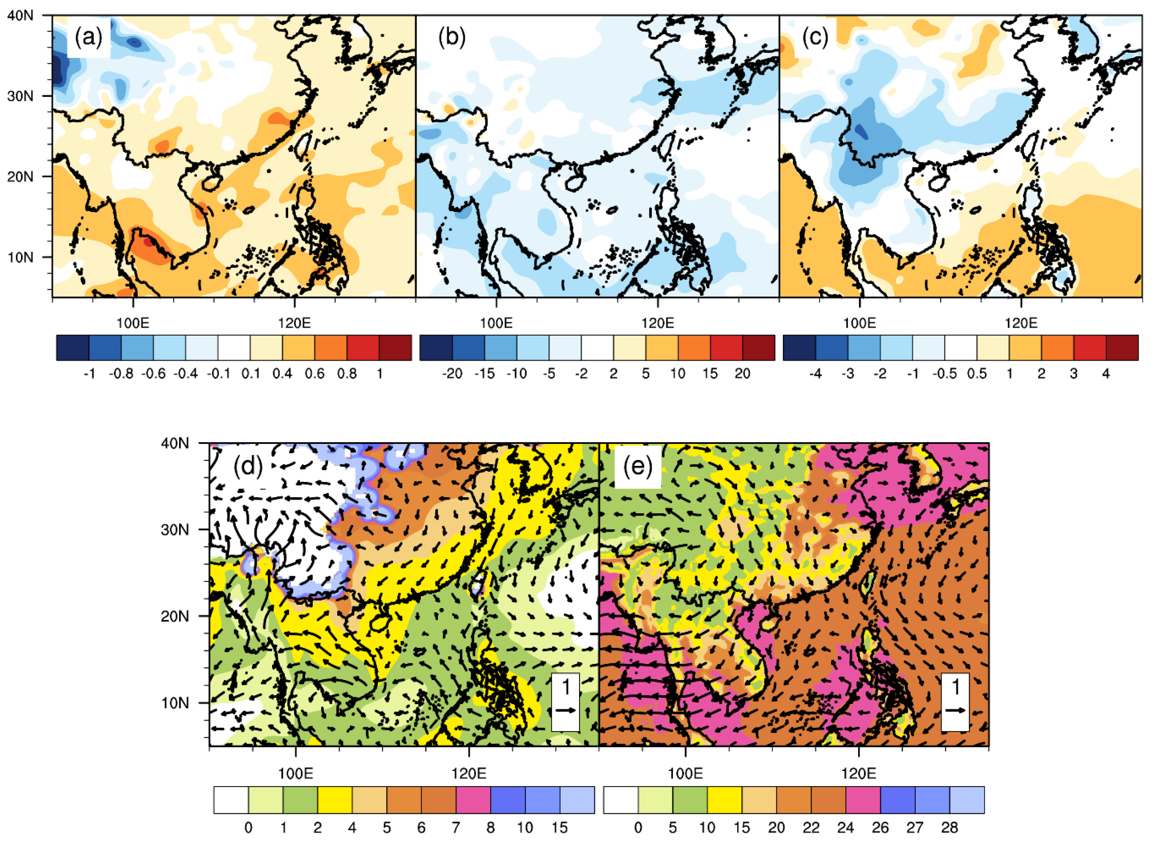
In Figure 2, the distributions of the deviations between simulation and reanalysis dataset are illustrated. The first row (Figure 2a–c) indicates the differences in the JJA average specific humidity at 700 hPa, precipitation rate and temperature at 2 m, respectively. The simulated specific humidity errors were relatively larger over China, especially over South China. However, the magnitude was almost negligible (around 10−4 kg/kg). The precipitation rate was generally smaller in the model than in reanalysis data. The temperature deviated slightly, in a range from −1 K to 1 K, over most China, except the Tibetan Plateau region. The second row indicates the deviations on the geopotential height and wind at 850 hPa and 500 hPa, respectively. The geopotential heights at both layers were generally overestimated in the model, with regional averaged extents of around 0.299% and 0.336% at 850 hPa and 500 hPa, respectively. It can be seen from Figure 2d,e that in the simulation, there were northeasterly wind anomalies at low layer and northwesterly wind anomalies at high layer over South China. The wind deviation was relatively large over the Tibetan Plateau region, which to a certain extent explains the specific humidity deviation over there as well. This is consistent with the negative deviation of precipitation, since the major water vapor sources over South China originate mainly from the Indian Ocean and the South China Sea (SCS) [34].
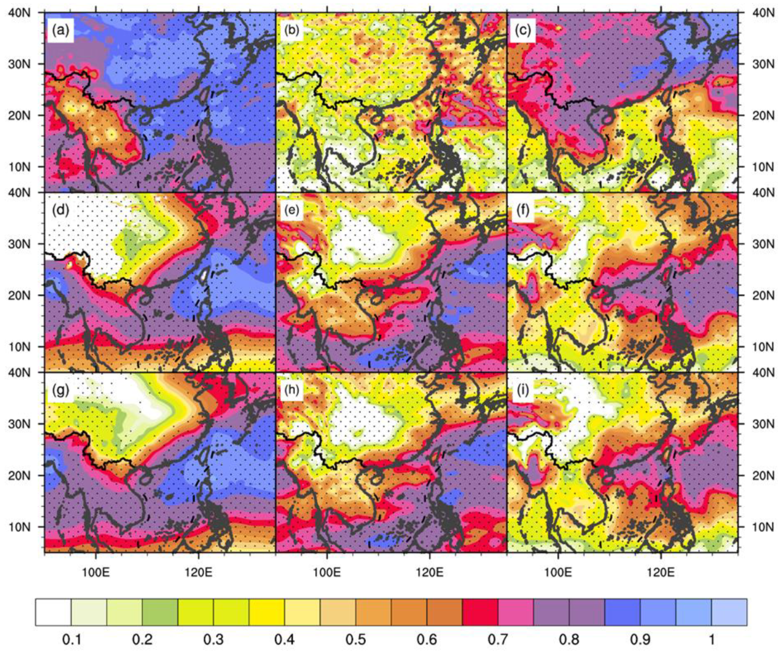
To further evaluate the simulation performance on a temporal scale, the ACC was computed based on the CTL test result and ERA5 reanalysis dataset at a time interval of 3 h. Figure 3 presents the distributions of ACC on the same variables as illustrated in Figure 2. The dotted area passed the significant test at a level of 90%. For the convenience of discussion, the confidence level was chosen in consideration of the spatial consistence and sample number of the results. The simulation performance on precipitation rate (Figure 3b) was relatively poorer than other variables, while those of specific humidity at 700 hPa (Figure 3a) and temperature at 2 m (Figure 3c) had the best performance among all. The simulations of geopotential height and wind were relatively consistent with reanalysis data temporally over South China (above 0.6).
Overall, the model reproduced well the major characteristics of the fundamental meteorological fields both spatially and temporally, which provides certain reliability for the following analysis.

3.2. Characteristerics of the Large-Scale Circulation in Summer 2015 under El Niño

As one of the main drivers of the climate over East Asia, ENSO events could cause enormous anomalies in large-scale circulation. In summer 2015, China was also strongly influenced by the El Niño event. Therefore, to depict the characteristics of the large-circulation changes in summer 2015, this section presents the composite analysis of El Niño years and La Nina years, and the variance analysis in 2015.
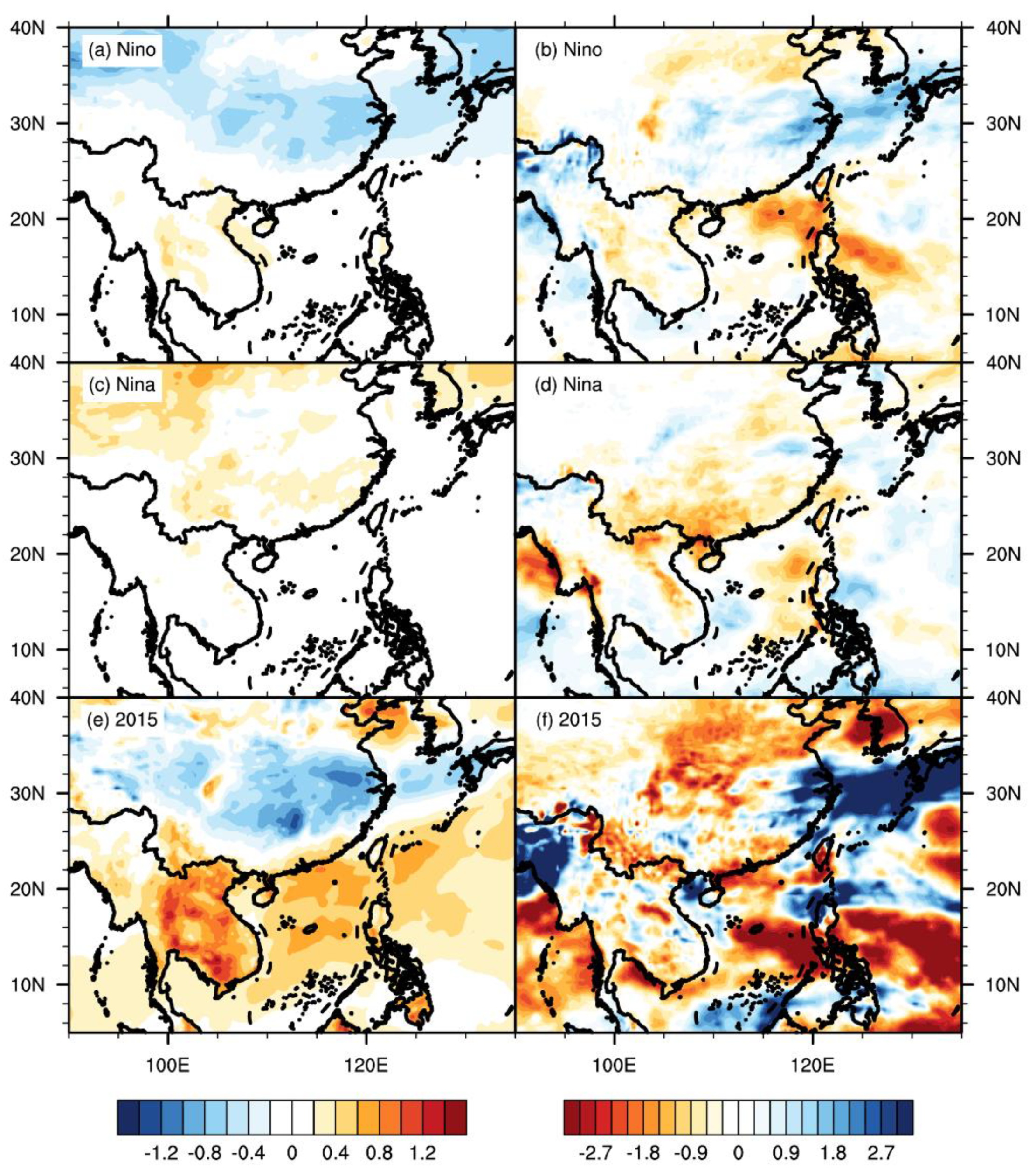
In Figure 4a–d, the composite analysis on JJA average temperature at 2m and precipitation rate in El Niño years and La Nina years are presented. An obvious inverse pattern between El Niño and La Nina was shown over China. Under El Niño (La Nina), the temperature over China was relatively lower (higher) while the precipitation rate was relatively higher (lower), particularly over East China. In Figure 4e,f, anomalies in 2015 were similar to those in Figure 4a,b, the mean state of El Niño years, but with a larger magnitude. The precipitation rate was higher over East China and lower over South China. As two regions incurring strong El Niño signal, they will be further discussed separately in the following sections.
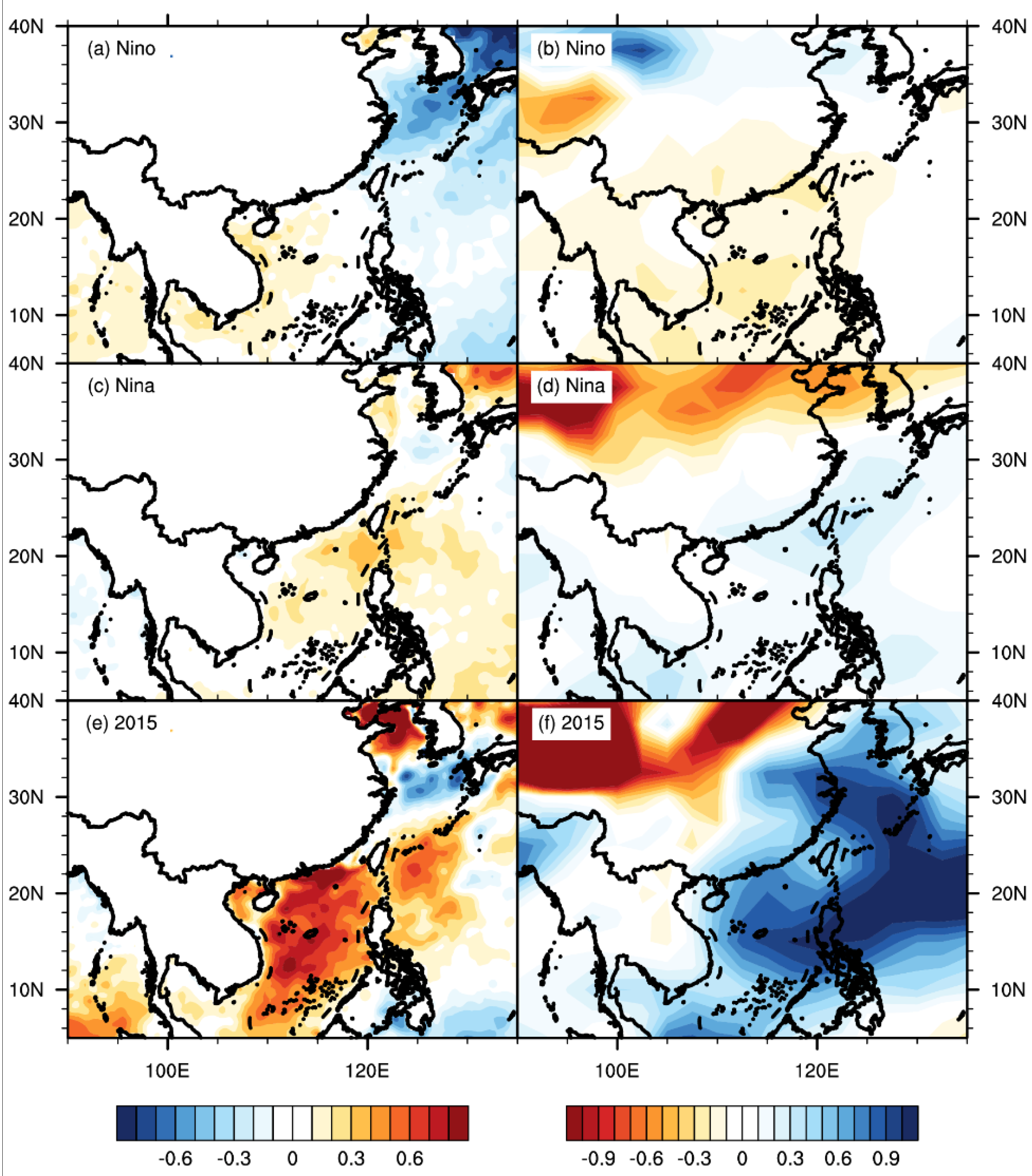
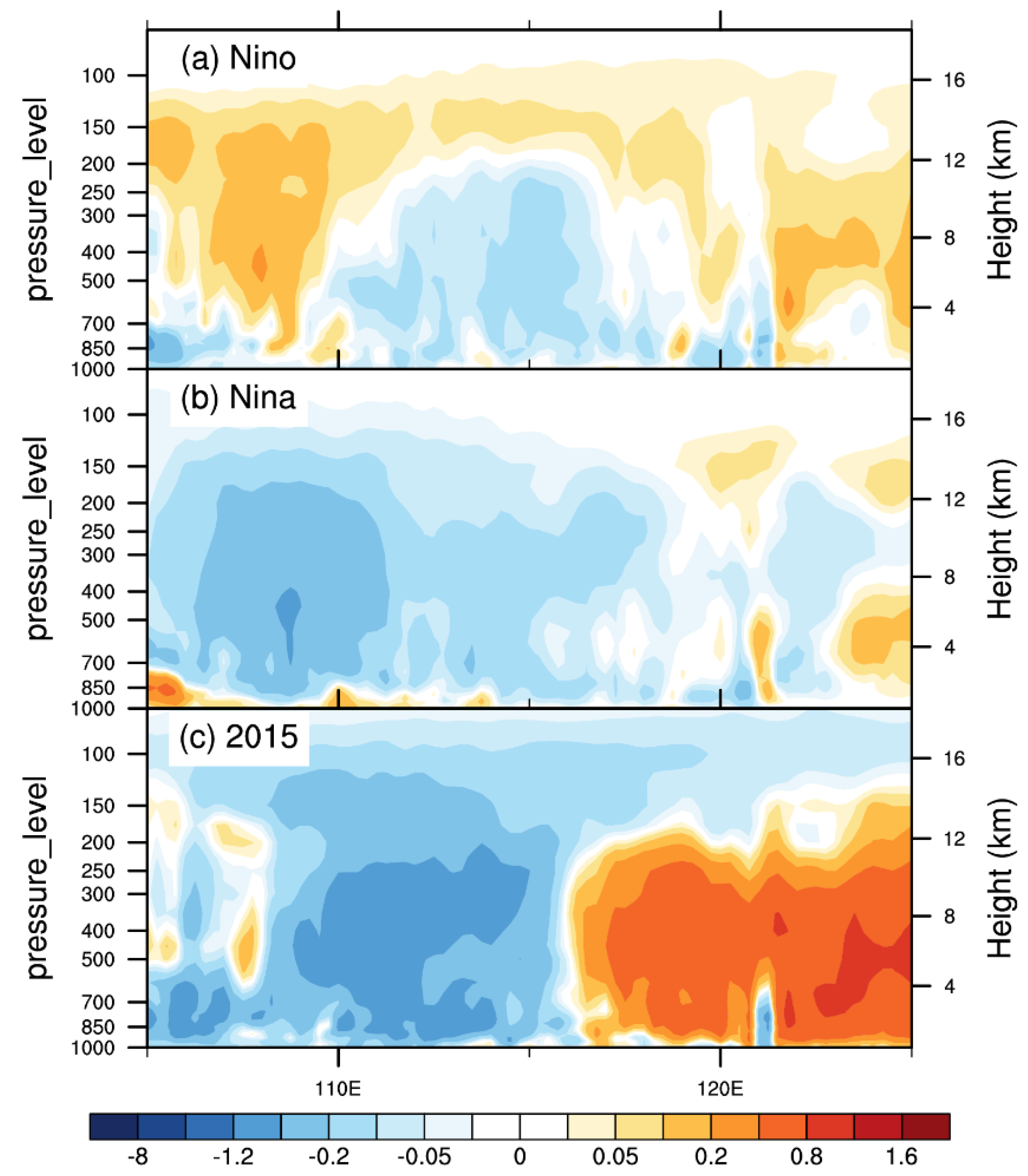
Figure 5 is same as Figure 4 but for anomalies of SST and 700-hPa specific humidity. In El Niño years, SST is relatively warmer over the Bay of Bengal, the west of SCS and the West Pacific Ocean, and cooler over the East Pacific Ocean. In La Nina years, the Pacific Ocean is mainly dominated with positive SST anomalies, especially over the east of SCS. In 2015, the positive anomalies over SCS were stronger. Compared with the mean state of El Niño, it was warmer over South China and cooler over East China. Influenced by the positive SST anomalies and the western Pacific subtropical high over the east, strong positive anomalies of specific humidity were seen over these two regions as well. It implies that the relatively higher temperature over SCS led to larger water vapor transport to East China, resulting in positive specific humidity anomalies. It can be seen from Figure 6a that there were abnormal upward motions over 105°–110° E and the West Pacific Ocean (120°–125° E) while downward motions over 110°–120° E under El Niño condition. By contrast, under La Nina condition, the area from 105° E to 120° E was dominated by downward motion anomalies, especially over South China (105°–110° E). Figure 6c shows that South China (105°–120° E) was dominated by the downward motion anomaly. However, East China (110°–125° E) was influenced by both downward motion and upward motion anomalies, which was in favor of circulation changes transporting water vapor from the Pacific Ocean and further enhancing the precipitation. This is consistent with the positive anomalies of precipitation rate over East China illustrated in Figure 4f.
Overall, the summertime anomalies in El Niño years and La Nina years exhibited distinct inverse patterns. El Niño caused cooling on land, especially over South China. Its impact on temperature showed a land-sea difference. Meanwhile, El Niño induced a decrease over South China and an increase over East China on precipitation. The distributions of the anomalies in 2015 resembled those in El Niño years but the magnitudes were larger. Stronger specific humidity anomalies in 2015 over East China and the Pacific Ocean indicated that positive SST anomalies over SCS and vertical circulation anomalies enhanced water vapor transport and subsequent convergence, especially over East China. In short, summer 2015 overall showed a stronger signal than the mean states of El Niño events.

3.3. Aerosol Direct Effect Impact on Precipitation

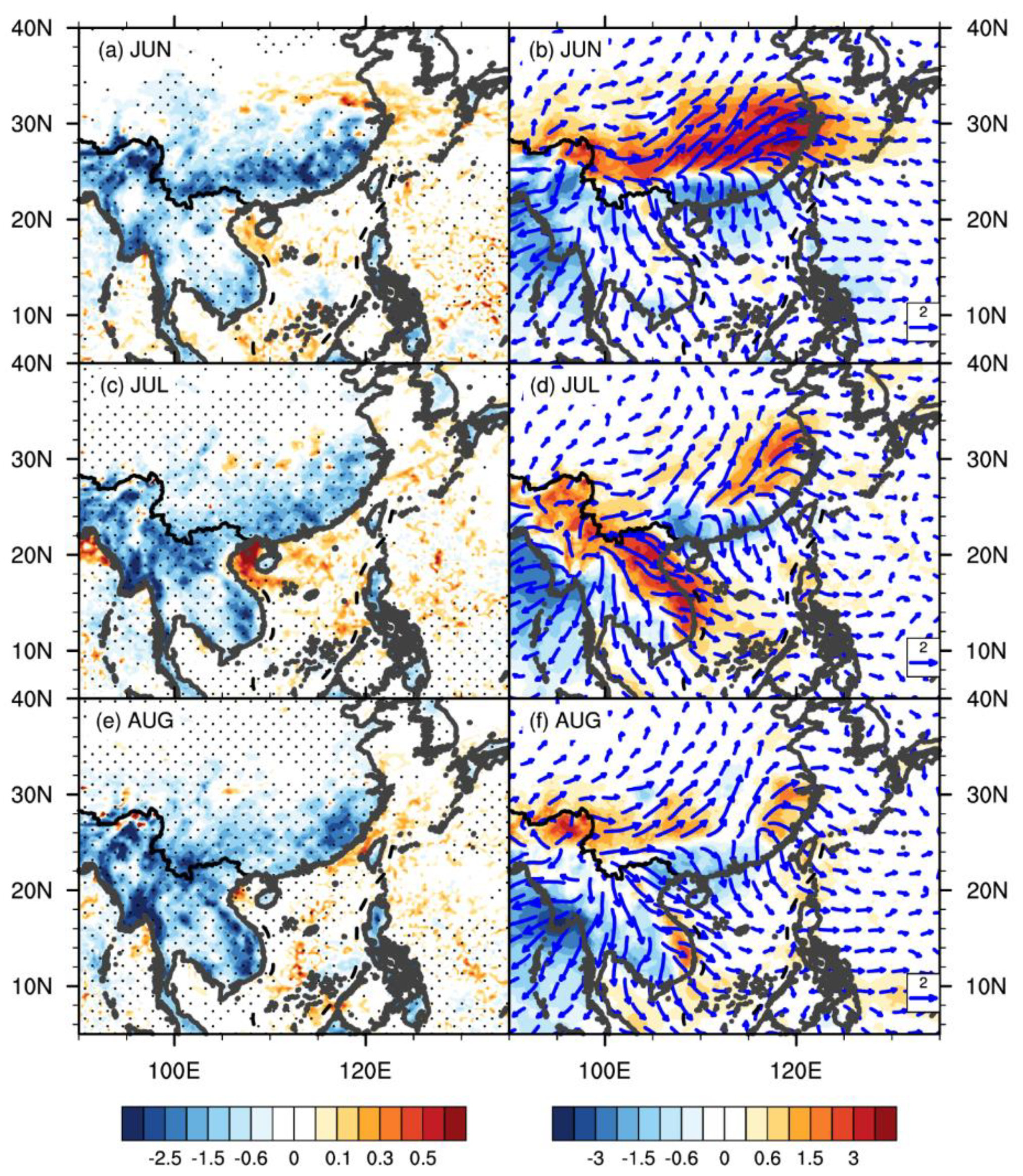
To examine the ADE, the differences between CTL and SEN test are presented in this section. Figure 7 shows the monthly average differences (CTL–SEN) in precipitation and water vapor fluxes. The anomalies of precipitation rate show obvious contrasts between land and sea, characterized by negative anomalies on land and relatively small positive anomalies over the sea. The domain average of precipitation rate reduction was −0.236 mm/day due to ADE. South China was one of the areas showing large anomalies, which passed the significant test at a level of 90%. From June to August, the distribution of precipitation rate differences remained similar with a decreasing trend over South China. In June, slight positive precipitation rate anomalies were seen over East China. In Figure 7b,d,f, water vapor transport anomalies were significantly different over South China and East China. Over South China, the water vapor flux anomalies were mainly transported by anomalous dry northerly winds, opposing the climatological water vapor originating from the SCS, the Indian Ocean and the Pacific Ocean [28]. Therefore, there were water vapor divergence anomalies leading to a precipitation decrease. By contrast, southwesterly water vapor flux anomalies prevailed over East China, which were especially strong in June and decreased in July and August.
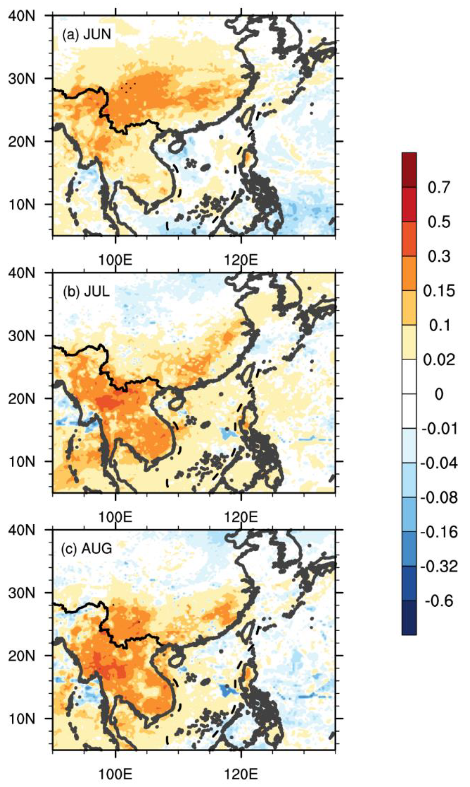
Summer is the season with relatively large aerosol optical depth (AOD), especially over areas with high urbanization and population such as South China and East China [35]. Figure 8 exhibits the difference in AOD (550 nm) due to ADE. Positive values indicate that AOD was higher in the CTL test than in the SEN test, which means the ADE increased AOD. In most of China, the ADE caused an increase in AOD, especially over the south showing a positive feedback [36]. The ADE induced an increase in AOD by 0.0285 on domain average. However, over North China, there existed a slight weakening effect. This implies that, the ADE was more significant over the populated areas with high aerosol emission. The distribution of the AOD difference is consistent with precipitation rate difference and its variation from June to August (Figure 7a,c,e).
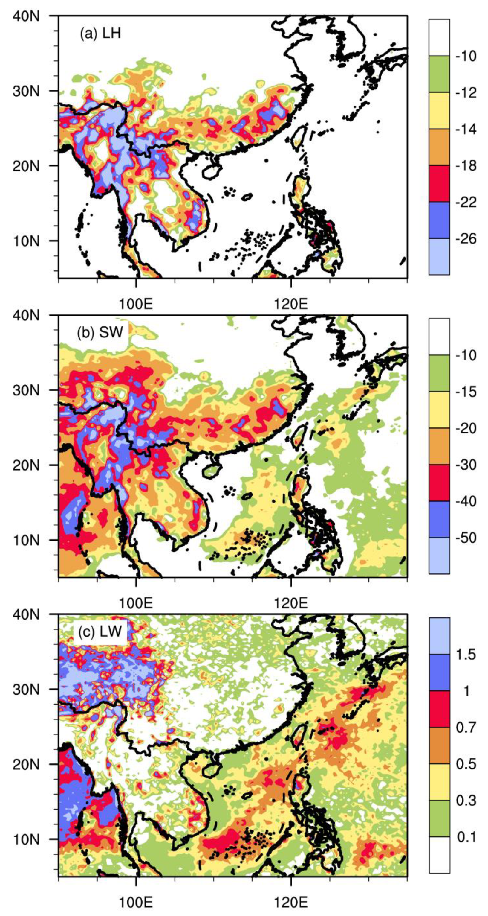
As ADE occurs mainly via the interactions of aerosol with radiation, the differences in latent heat flux (LH), downward shortwave radiation flux (SW) and downward longwave flux (LW) are summarized in Figure 9. ADE induced decreases in LH and SW and increases in LW. The scattering and absorbing effect of aerosol led to weakened SW, and further decreased LH. The domain average variations due to ADE were −2.855, −11.606, and 0.290 W/m2 for LH, SW, and LW, respectively. Most of the solar radiation absorbed by the ground surface (60–70%) was consumed via evaporation. The distributions of the changes in LH and SW showed land-sea difference similar to that of precipitation changes (Figure 7a,c,e), mainly over South and West China, which means ADE influenced the precipitation mainly through aerosol-radiation interaction. Considering the changes in temperature in Figure 4a,e, ADE was in phase with the El Niño impact over South China. The decrease in LH means weakened evaporation processes, which might suppress precipitation. The enhancing impact on LW due to ADE was relatively small compared with that on SW. However, ADE was, overall, in favor of a more stable atmosphere.
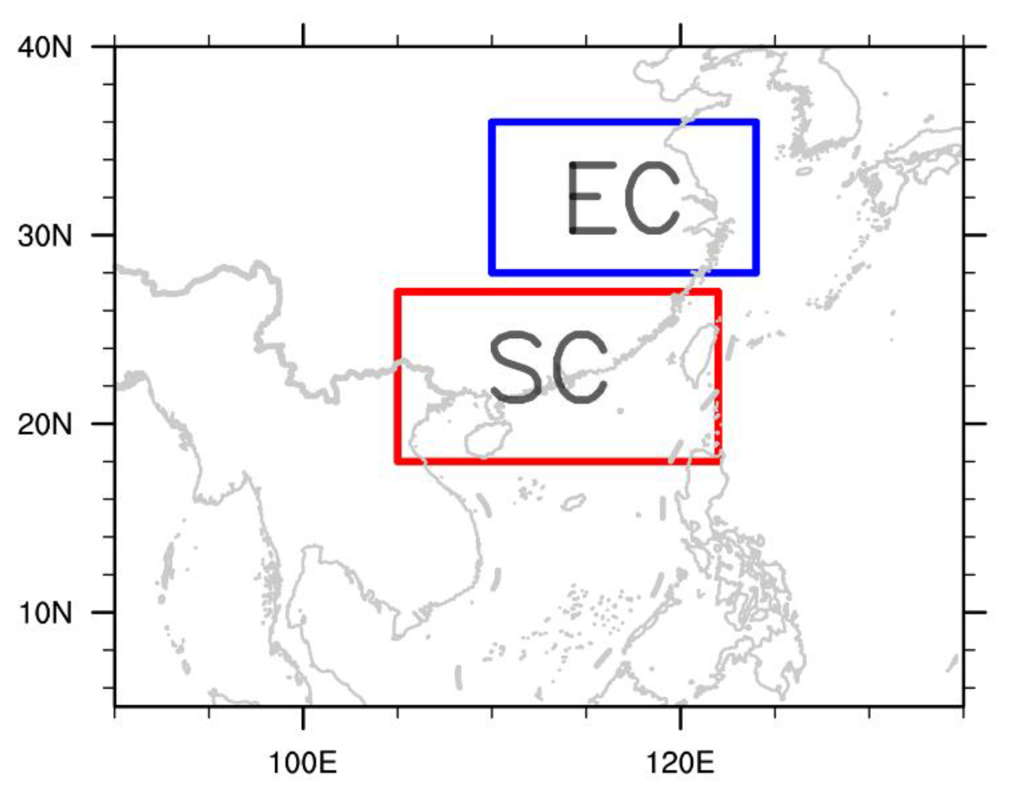
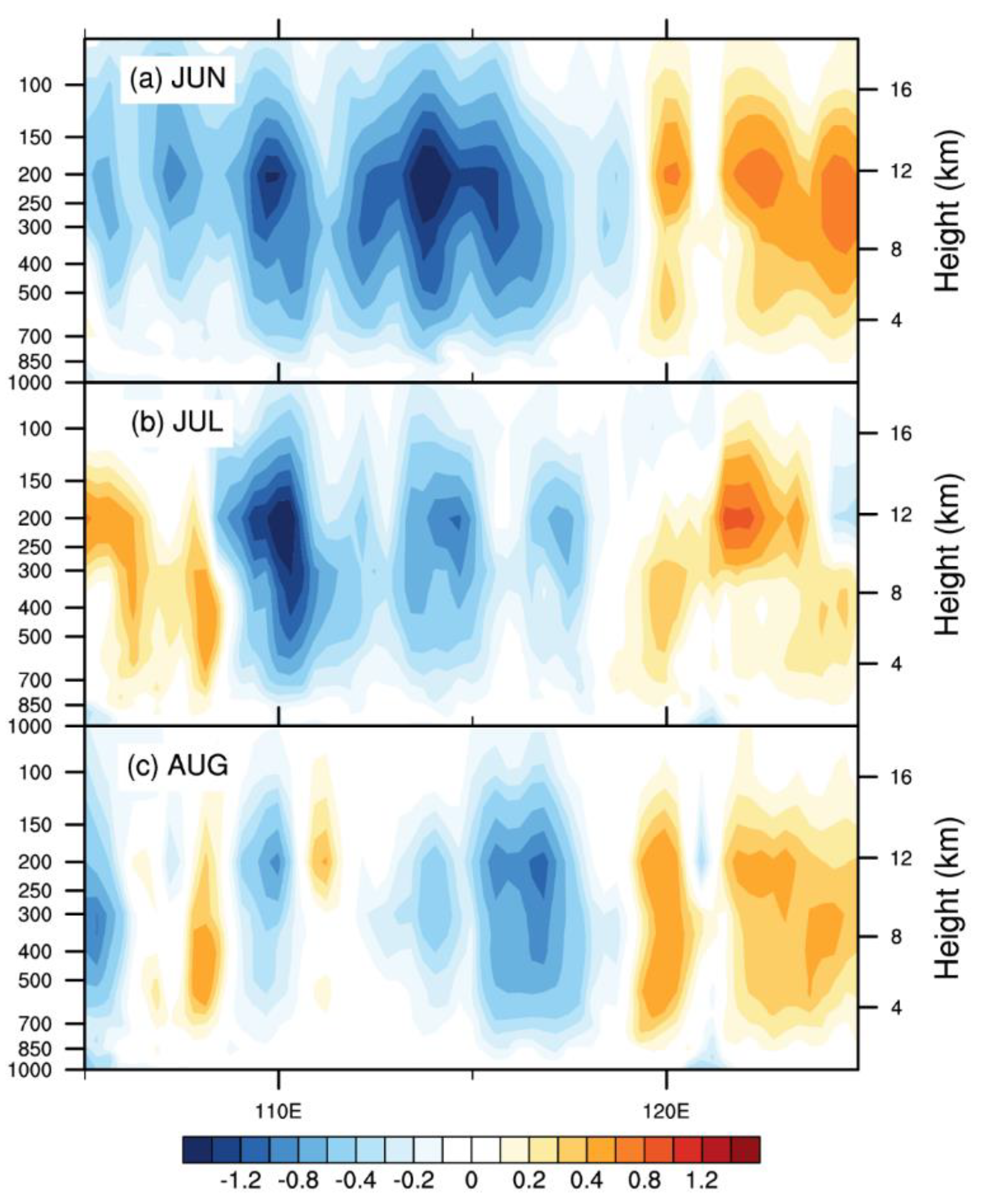
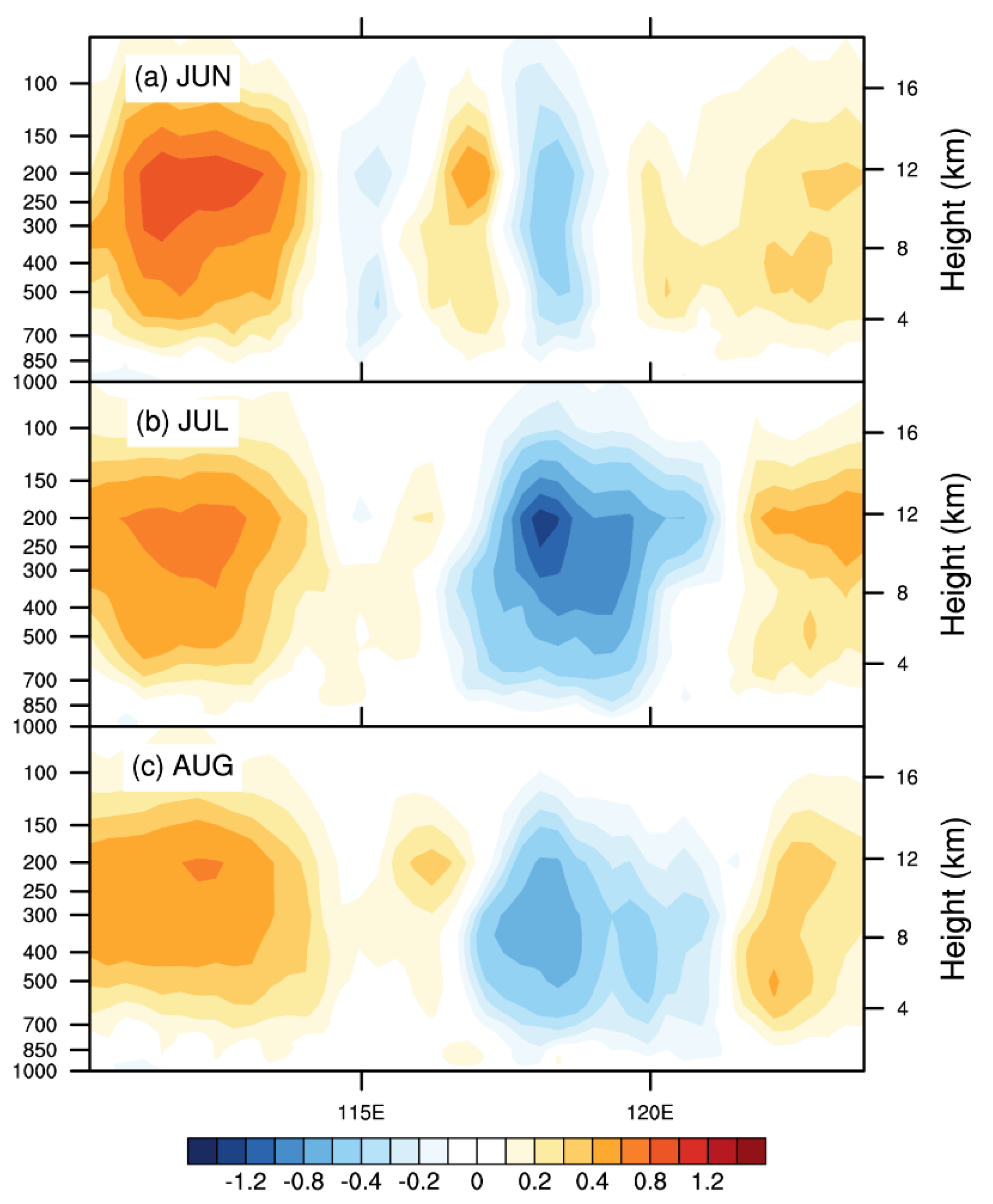
To better investigate the spatial variation of ADE, we select EC (East China; 28–36° N, 110–124° E) and SC (South China; 18–27° N, 105–122° E) as shown in Figure 10. Figure 11 and Figure 12 show the difference in vertical velocity due to ADE. Positive (negative) values indicate upward (downward) motion. In SC region, the vertical velocity anomalies induced by ADE were mostly downward motion, with stronger intensity in June. Circulation anomaly in favor of water vapor transport occurred in July and August, which was consistent with the weakening in the ADE-induced precipitation rate decrease (Figure 7c,e). However, it was relatively weak compared to effect on the radiation change.
In summary, ADE caused a reduction in precipitation rate and an increase in AOD over most of China. Interestingly, we found that the mechanism of ADE may differ over SC and EC regions. In SC, ADE caused stronger precipitation rate decrease (−0.646 mm/day) than that in EC (−0.240 mm/day). The water vapor flux was suppressed by ADE (−0.151 kg m−1 s−1) rather than enhanced (0.832 kg m−1 s−1) in EC. The radiation forcing was stronger than that in EC. SW was reduced by 16.659 W/m2 and 9.312 W/m2 averaged over SC and EC in JJA, respectively. LH was reduced by 7.678 W/m2 and 4.166 W/m2 averaged over SC and EC in JJA, respectively. LW changes were relatively insignificant over both regions. In SC, ADE decreased the shortwave radiation via scattering and absorbing effects, which cooled the region in phase with El Niño impact. This might result in increases in the pressure over land and a pressure gradient pointing from land to ocean. As a consequence, the water vapor transport towards SC was weakened in spite of the positive specific humidity anomalies in summer of 2015. This resulted in a more stable atmosphere that suppressed precipitation. In EC (Figure 12), besides the absorbing effect, ADE also enhanced the vertical circulation anomaly in contrast to that caused by the El Niño effect, which further suppressed precipitation. The suppressing effect was enhanced from June to August.

4. Conclusions and Discussion

In this study, two simulations were conducted using the WRF-Chem V3.5.1 model, with (CTL) and without (SEN) aerosol-radiation interaction. The differences between two tests were used to estimate ADE. We focused on two regions, South China and East China, which have high aerosol aerosols due to rapid urbanization and large populations. Although several publications have investigated ADE over China, few studies discuss the joint ENSO effect and ADE. With consideration of the specialty of the El Niño condition in summer 2015, ADE over China was studied and discussed above. Results of certain referential values are presented and can be summarized as follows:
  • As a strong El Niño event, summer 2015 showed similar signals as the mean state of El Niño years based on the composite analysis. The large-scale circulation changes of summer 2015 tended to induce cooling (warming) and wet (dry) conditions over East China (South China). Moreover, summer 2015 also showed additional features. For example, positive specific humidity anomalies were found over East China and the Pacific Ocean. This is because that the positive SST anomalies over SCS enhanced the water vapor transport eastwards. In addition, the upward motion anomalies over the West Pacific Ocean and downward motion anomalies over East China enhanced the circulation and water vapor transport from the ocean. However, the upward motion anomalies were relatively small over South China.
  • Including aerosol effect and their related physical and chemical processes, the CTL test reproduced well the main characteristics of the fundamental meteorological fields based on comparing with reanalysis.
  • ADE on precipitation rate showed obvious land-sea differences to those on SW. Over China, they were mainly negative, especially over SC. Aerosol scattering and absorbing effects led to decreases in SW and increases in LW, which further led to a weakened LH, a more stable atmosphere and a weakened water cycle.
  • The spatial heterogeneity of ADE was discussed. The water vapor transport was suppressed due to ADE over SC (−0.151 kg m−1 s−1) while strongly enhanced over EC (0.832 kg m−1 s−1). SW reduction due to ADE was more significant over SC (16.659 W/m2) than over EC (9.312 W/m2). This implies that aerosol radiative forcing was relatively stronger over SC than over EC.
  • In SC, ADE-induced precipitation reduction was mainly caused by radiative forcing and weakened water vapor transport, which enhanced atmospheric stability. The cooling effect of aerosol was consistent with the El Niño effect over SC. In EC, ADE-induced precipitation reduction was related to the vertical circulation anomalies that were contradictory with those caused by El Niño effect.
The investigation was mainly focused on China and Southeast Asia. The universality of the results needs to be further tested. This study only discusses a case occurring in summer 2015. However, ADE during La Nina and the boreal winter is also of great significance. Moreover, aerosol indirect effect over China and its interaction with ENSO background could be another meaningful topic in our future study.

Author Contributions

Conceptualization, J.L.; methodology, J.L. and B.J.; software, F.L. and B.J.; validation, F.L.; formal analysis, F.L.; investigation, F.L.; resources, J.L. and W.L.; data curation, F.L.; writing—original draft preparation, F.L.; writing—review and editing, J.L. and W.L.; visualization, F.L.; supervision, J.L. and W.L.; project administration, J.L. and W.L.; funding acquisition, W.L. All authors have read and agreed to the published version of the manuscript.

Funding

The study is funded by the National Key Research and Development Program of China [2018YFC1507402], National Natural Science Foundation of China (Grant No. 41875168 and No. 42075064), and Guangzhou Science and Technology Plan (201707010088).

Institutional Review Board Statement

Not applicable.

Informed Consent Statement

Not applicable.

Data Availability Statement

Data available in a publicly accessible repository that does not issue DOIs. Publicly available da-tasets were analyzed in this study. This data can be found here: https://rda.ucar.edu/datasets/ds083.2/; http://retro.enes.org; https://cds.climate.copernicus.eu/cdsapp#!/home.

Acknowledgments

We sincerely appreciate the free reanalysis datasets provided by National Centers for Environmental Prediction (NCEP), European Centre for Medium-Range Weather Forecasts (ECMWF), and National Center for Atmospheric Research (NCAR).

Conflicts of Interest

The authors declare no conflict of interest.

References

  1. Boucher, O.; Tanré, D. Estimation of the aerosol perturbation to the Earth’s Radiative Budget over oceans using POLDER satellite aerosol retrievals. Geophys. Res. Lett. 2000, 27, 1103–1106. [Google Scholar] [CrossRef]
  2. Carslaw, K.S.; Boucher, O.; Spracklen, D.V.; Mann, G.W.; Rae, J.G.L.; Woodward, S.; Kulmala, M. A review of natural aerosol interactions and feedbacks within the Earth system. Atmos. Chem. Phys. 2010, 10, 1701–1737. [Google Scholar] [CrossRef] [Green Version]
  3. Heald, C.L.; Ridley, D.A.; Kroll, J.H.; Barrett, S.R.H.; Cady-Pereira, K.E.; Alvarado, M.J.; Holmes, C.D. Contrasting the direct radiative effect and direct radiative forcing of aerosols. Atmos. Chem. Phys. 2014, 14, 5513–5527. [Google Scholar] [CrossRef] [Green Version]
  4. Andreae, M.O.; Rosenfeld, D. Aerosol–cloud–precipitation interactions. Part 1. The nature and sources of cloud-active aerosols. Earth-Sci. Rev. 2008, 89, 13–41. [Google Scholar] [CrossRef]
  5. Ghan, S.J.; Liu, X.; Easter, R.C.; Zaveri, R.; Rasch, P.J.; Yoon, J.-H.; Eaton, B. Toward a Minimal Representation of Aerosols in Climate Models: Comparative Decomposition of Aerosol Direct, Semidirect, and Indirect Radiative Forcing. J. Clim. 2012, 25, 6461–6476. [Google Scholar] [CrossRef]
  6. Ghan, S.J. Technical Note: Estimating aerosol effects on cloud radiative forcing. Atmos. Chem. Phys. 2013, 13, 9971–9974. [Google Scholar] [CrossRef] [Green Version]
  7. Huang, X.; Song, Y.; Zhao, C.; Cai, X.; Zhang, H.; Zhu, T. Direct Radiative Effect by Multicomponent Aerosol over China. J. Clim. 2015, 28, 3472–3495. [Google Scholar] [CrossRef]
  8. Li, J.; Yang, Y.; Li, F.; Lin, W. Simulated influence of air pollution and aerosols on summer precipitation over the Pearl River Delta region. Meteorol. Z. 2020, 29, 41–53. [Google Scholar] [CrossRef]
  9. Zhou, M.; Zhang, L.; Chen, D.; Gu, Y.; Fu, T.M.; Gao, M.; Zhao, B. The impact of aerosol-radiation interactions on the effectiveness of emission control measures. Environ. Res. Lett. 2019, 14, 024002. [Google Scholar] [CrossRef]
  10. Abish, B.; Mohanakumar, K. Absorbing aerosol variability over the Indian subcontinent and its increasing dependence on ENSO. Glob. Planet. Chang. 2013, 106, 13–19. [Google Scholar] [CrossRef]
  11. Chang, L.; Xu, J.; Tie, X.; Wu, J. Impact of the 2015 El Niño event on winter air quality in China. Sci. Rep. 2016, 6, 1–6. [Google Scholar] [CrossRef] [PubMed]
  12. Kim, M.; Lau, W.K.M.; Kim, K.-M.; Sang, J.; Kim, Y.H.; Lee, W.-S. Amplification of ENSO effects on Indian summer monsoon by absorbing aerosols. Clim. Dyn. 2016, 46, 2657–2671. [Google Scholar] [CrossRef] [Green Version]
  13. Bellouin, N.; Boucher, O.; Haywood, J.; Reddy, M.S. Global estimate of aerosol direct radiative forcing from satellite measurements. Nature 2005, 438, 1138–1141. [Google Scholar] [CrossRef] [PubMed]
  14. Grell, G.A.; Peckham, S.E.; Schmitz, R.; McKeen S., A.; Frost, G.; Skamarock, W.C.; Eder, B. Fully coupled “online” chemistry within the WRF model. Atmos. Environ. 2005, 39, 6957–6975. [Google Scholar] [CrossRef]
  15. Skamarock, W.C.; Klemp, J.B.; Dudhia, J.; Gill, D.O.; Barker, D.M.; Duda, M.G.; Huang, X.-Y.; Wang, W.; Powers, J.G. A description of the advanced research WRF version 3. In NCAR Technical Note; National Center for Atmospheric Research: Boulder, CO, USA, 2008. [Google Scholar]
  16. Hong, S.Y.; Noh, Y.; Dudhia, J. A new vertical diffusion package with an explicit treatment of entrainment processes. Monthly Weather Rev. 2006, 134, 2318–2341. [Google Scholar] [CrossRef] [Green Version]
  17. Kain, J.S.; Fritsch, J.M. Convective parameterization for mesoscale models: The Kain–Fritsch scheme. The Representation of Cumulus Convection in Numerical Models. Amer. Meteor. Soc. 1993, 165–170. [Google Scholar]
  18. Iacono, M.J.; Delamere, J.S.; Mlawer, E.J.; Shephard, M.W.; Clough, S.A.; Collins, W.D. Radiative forcing by long-lived greenhouse gases: Calculations with the AER radiative transfer models. J. Geophys. Res. Atmos. 2008, 113. [Google Scholar] [CrossRef]
  19. Stockwell, W.R.; Middleton, P.; Chang, J.S.; Tang, X. The second generation regional acid deposition model chemical mechanism for regional air quality modeling. J. Geophys. Res. Atmos. 1990, 95, 16343–16367. [Google Scholar] [CrossRef]
  20. Ackermann, I.J.; Hass, H.; Memmesheimer, M.; Ebel, A.; Binkowski, F.S.; Shankar, U.M.A. Modal aerosol dynamics model for Europe: Development and first applications. Atmos. Environ. 1998, 32, 2981–2999. [Google Scholar] [CrossRef]
  21. Schell, B.; Ackermann, I.J.; Hass, H.; Binkowski, F.S.; Ebel, A. Modeling the formation of secondary organic aerosol within a comprehensive air quality model system. J. Geophys. Res. Atmos. 2001, 106, 28275–28293. [Google Scholar] [CrossRef]
  22. Morrison, H.; Pinto, J.O. Mesoscale modeling of springtime Arctic mixed-phase stratiform clouds using a new two-moment bulk microphysics scheme. J. Atmos. Sci. 2005, 62, 3683–3704. [Google Scholar] [CrossRef]
  23. Morrison, H.; Thompson, G.; Tatarskii, V. Impact of cloud microphysics on the development of trailing stratiform precipitation in a simulated squall line: Comparison of one- and two-moment schemes. Monthly Weather Rev. 2009, 137, 991–1007. [Google Scholar] [CrossRef] [Green Version]
  24. Peckham, S.E.; Grell, G.; McKeen, S.A.; Ahmadov, R.; Fast, J.D.; Gustafson, W.I.; Ghan, S.J.; Zaveri, R.; Easter, R.C.; Barnard, J. WRF-Chem Version 3.5.1 User’s Guide; National Oceanic and Atmospheric Administration: Washington, DC, USA, 2013. [Google Scholar]
  25. Du, Q.; Zhao, C.; Zhang, M.; Dong, X.; Chen, Y.; Liu, Z.; Hu, Z.; Zhang, Q.; Li, Y.; Yuan, R.; et al. Modeling diurnal variation of surface PM 2.5 concentrations over East China with WRF-Chem: Impacts from boundary-layer mixing and anthropogenic emission. Atmos. Chem. Phys. 2020, 20, 2839–2863. [Google Scholar] [CrossRef] [Green Version]
  26. Guo, J.; He, J.; Liu, H.; Miao, Y.; Liu, H.; Zhai, P. Impact of various emission control schemes on air quality using WRF-Chem during APEC China 2014. Atmos. Environ. 2016, 140, 311–319. [Google Scholar] [CrossRef]
  27. Meng, L.; Yang, X.; Zhao, T.; He, Q.; Lu, H.; Mamtimin, A.; Huo, W.; Yang, F.; Liu, C. Modeling study on three-dimensional distribution of dust aerosols during a dust storm over the Tarim Basin, Northwest China. Atmos. Res. 2019, 218, 285–295. [Google Scholar] [CrossRef]
  28. Wang, P.; Qiao, X.; Zhang, H. Modeling PM2. 5 and O3 with aerosol feedbacks using WRF/Chem over the Sichuan Basin, southwestern China. Chemosphere 2020, 254, 126735. [Google Scholar] [CrossRef]
  29. Wei, W.; Lv, Z.F.; Li, Y.; Wang, L.T.; Cheng, S.; Liu, H. A WRF-Chem model study of the impact of VOCs emission of a huge petro-chemical industrial zone on the summertime ozone in Beijing, China. Atmos. Res. 2018, 175, 44–53. [Google Scholar] [CrossRef]
  30. Copernicus Climate Change Service (C3S). ERA5: Fifth generation of ECMWF atmospheric reanalyses of the global climate. Copernicus Climate Change Service Climate Data Store (CDS). 2017. Available online: https://cds.climate.copernicus.eu/cdsapp#!/home (accessed on 28 December 2020).
  31. Joliffe, I.T.; Stephenson, D.B. Forecast Verification: A Practitioner’s Guide in Atmospheric Science; John Wiley and Son: New York, NY, USA, 2003; p. 240. [Google Scholar]
  32. Wang, Y.; Qian, H.; Song, J.-J.; Jiao, M.-Y. Verification of the T213 global spectral model of China National Meteorology Center over the East-Asia area. J. Geophys. Res. 2008, 113, 1–7. [Google Scholar] [CrossRef] [Green Version]
  33. Wolter, K.; Timlin, M.S. El Niño/Southern Oscillation behaviour since 1871 as diagnosed in an extended multivariate ENSO index (MEI. ext). Int. J. Climatol. 2011, 31, 1074–1087. [Google Scholar] [CrossRef]
  34. Li, F.; Lin, W.; Li, J. ENSO-related impact on the vapor sources of China based on case simulations of summer 2015 and 2010. J. Atmos. Sol. Terr. Phys. 2020, 211, 105489. [Google Scholar] [CrossRef]
  35. De Leeuw, G.; Sogacheva, L.; Rodriguez, E.; Kourtidis, K.; Georgoulias, A.K.; Alexandri, G.; Amiridis, V.; Proestakis, E.; Marinou, E.; Xue, Y.; et al. Two decades of satellite observations of AOD over mainland China using ATSR-2, AATSR and MODIS/Terra: Data set evaluation and large-scale patterns. Atmos. Chem. Phys. 2018, 18, 1573. [Google Scholar] [CrossRef] [Green Version]
  36. Liu, Z.; Yim, S.H.; Wang, C.; Lau, N.C. The impact of the aerosol direct radiative forcing on deep convection and air quality in the Pearl River Delta region. Geophys. Res. Lett. 2018, 45, 4410–4418. [Google Scholar] [CrossRef]
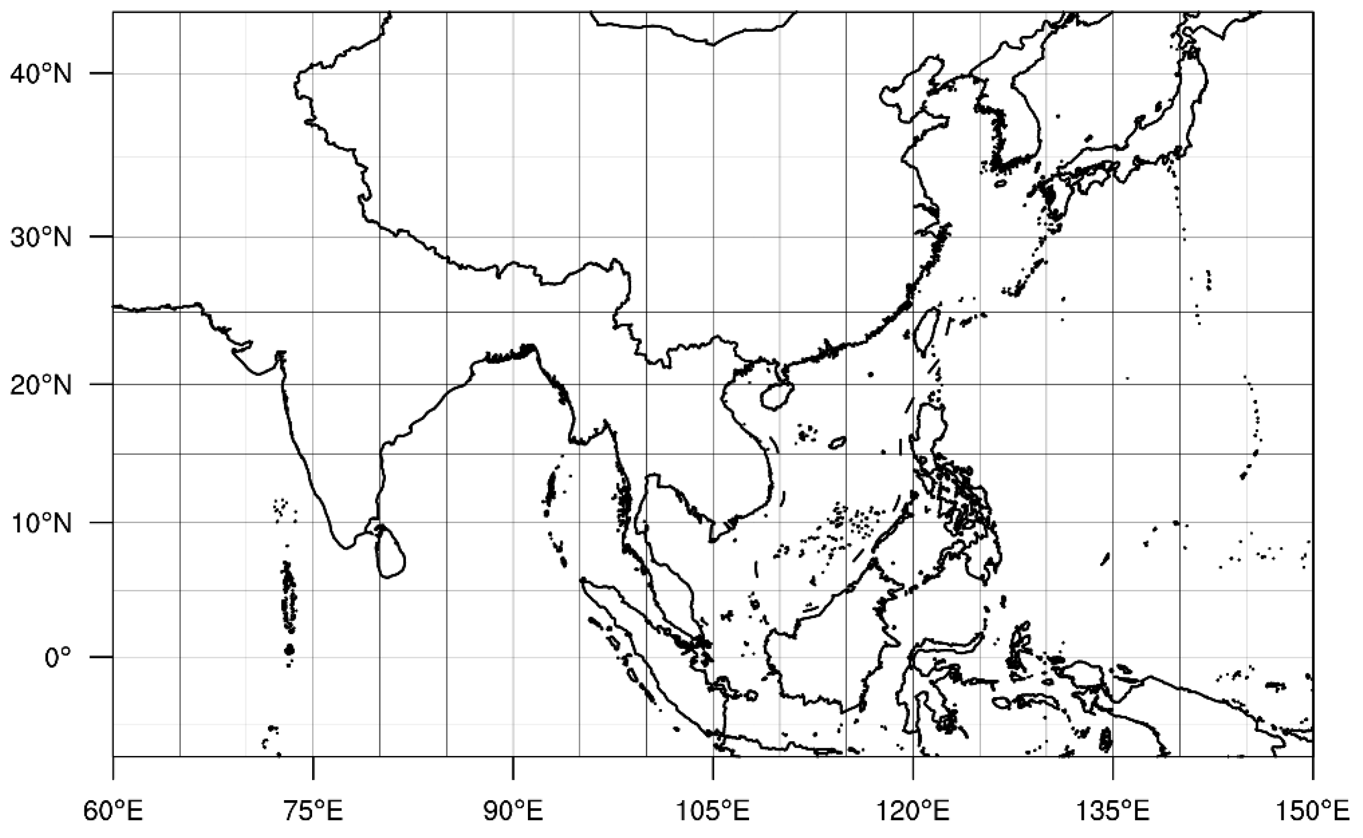
Figure 1. The simulated region (60° W–150° E, 5° S–45° N).
Atmosphere 12 00058 g001
Figure 2. Differences between simulation from CTL test and ERA5 reanalysis datasets averaged from June to August 2015 on (a) specific humidity at 700 hPa (unit: 10−3 kg/kg), (b) precipitation rate (unit: mm/day), (c) temperature at 2 m (unit: K), (d) the geopotential height (contour; unit: gpm) and wind (vector; unit: m/s) at 850 hPa, and (e) 500 hPa.
Atmosphere 12 00058 g002
Figure 3. The temporal ACC (contour) of simulation from CTL test and ERA5 reanalysis datasets on (a) specific humidity at 700 hPa (unit: 10−3 kg/kg), (b) precipitation rate (unit: mm/day), (c) temperature at 2 m (unit: K), (d,g) the geopotential height (unit: gpm), (e,h) zonal wind, and (f,i) meridional wind at 850 hPa (the second row) and 500 hPa (the third row). Dotted area indicate that the values passed the significant test at a level of 90%.
Atmosphere 12 00058 g003
Figure 4. Average temperature at 2m (left; unit: K) and precipitation rate (right; unit: mm/day) anomalies of JJA in (a,b) El Niño years, (c,d) La Nina years, and (e,f) 2015 from ERA5 reanalysis datasets.
Atmosphere 12 00058 g004
Figure 5. Average sea surface temperature (left; unit: K) and specific humidity at 700 hPa (right; unit: kg/kg) anomalies of JJA in (a,b) El Niño years, (c,d) La Nina years, and (e,f) 2015 from ERA5 reanalysis datasets.
Atmosphere 12 00058 g005
Figure 6. JJA average anomalies of the zonal mean vertical velocity (unit: Pa/s; the values are increased by −50 times) from 20° N–30° N in (a) El Niño years, (b) La Nina years, and (c) 2015 from ERA5 reanalysis datasets. Left axis stands for pressure levels (unit: hPa) and right axis stands for the height (unit: km).
Atmosphere 12 00058 g006
Figure 7. Monthly average differences due to ADE (CTL-SEN test) in precipitation rate (unit: mm/day; dotted area indicate that the values passed the significant test at a level of 90%.) on (a) June, (c) July, and (e) August; and in the vertical integral of moisture flux (vector; unit: kg m−1 s−1) and its absolute value (contour; unit: kg m−1 s−1) on (b) June, (d) July, and (f) August.
Atmosphere 12 00058 g007
Figure 8. Monthly average difference in aerosol optical depth (AOD, 550 nm) due to ADE (CTL-SEN test) on (a) June, (b) July, and (c) August.
Atmosphere 12 00058 g008
Figure 9. JJA average differences (unit: W/m2) due to ADE (CTL-SEN test) in (a) latent heat flux, (b) downward shortwave radiation flux, and (c) downward longwave radiation flux.
Atmosphere 12 00058 g009
Figure 10. Selected regions. Red box (18–27° N, 105–122° E) indicates SC, South China; blue box indicates EC (28–36° N, 110–124° E), East China.
Atmosphere 12 00058 g010
Figure 11. Monthly average difference due to ADE (CTL-SEN test) in the zonal mean vertical velocity (unit: m/s) over SC region on (a) June, (b) July, and (c) August. Left axis stands for pressure levels (unit: hPa) and right axis stands for the height (unit: km).
Atmosphere 12 00058 g011
Figure 12. Same as Figure 11 but over EC region.
Atmosphere 12 00058 g012
Table 1. WRF-Chem configuration options for the experiment. YSU, Yonsei University; RADM2, Regional Acid Deposition Model version 2.
Atmospheric ProcessWRF-Chem Option
Cloud microphysicsMorrison scheme
Longwave and shortwave radiationRapid Radiative Transfer Model
Surface layerMonin-Obukhov scheme
Land surface modelNoah Land-Surface model
Planetary boundary layerYSU scheme
CumulusKain–Fritsch scheme
PhotolysisFast-J photolysis
Gas phase chemistryRADM2
Aerosol chemistryMADE/SORGAM including some aqueous reactions
Anthropogenic emissionsRETRO
Table 2. Experimental design.
TestDescriptionNamelist Options
CTLControl experiment including aerosol effect.aer_ra_feedback = 1
SENSame as CTL except excluding ADE.aer_ra_feedback = 0
Table 3. Evaluation of the simulated meteorological fields (average fields from June to August 2015). NRMSE: normalized root mean square error.
Variables (Unit)Pattern Correlation 1NRMSE1
Temperature at 2 m (K)0.9980.0002
Specific humidity (kg/kg)0.9990.0002
Precipitation rate (mm/day)0.7920.0032
Geopotential height at 850 hPa (gpm)0.7820.00006
Geopotential height at 500 hPa (gpm)0.9870.00002
U wind at 850 hPa (m/s)0.9930.0012
V wind at 850 hPa (m/s)0.9710.0022
U wind at 500 hPa (m/s)0.9910.0012
V wind at 500 hPa (m/s)0.9620.0180
1 The pattern correlations passed the significant test at a level of 99%. 2 NRMSE stands for the normalized root mean square error.
Publisher’s Note: MDPI stays neutral with regard to jurisdictional claims in published maps and institutional affiliations.