High–Resolution Modeling of Airflows and Particle Deposition over Complex Terrain at Sakurajima Volcano

Abstract

The realistic representation of atmospheric pollutant dispersal over areas of complex topography presents a challenging application for meteorological models. Here, we present results from high–resolution atmospheric modeling in order to gain insight into local processes that can affect ash transport and deposition. The nested Weather Research and Forecasting (WRF) model with the finest resolution of 50 m was used to simulate atmospheric flow over the complex topography of Sakurajima volcano, Japan, for two volcanic eruption cases. The simulated airflow results were shown to compare well against surface observations. As a preliminary application, idealized trajectory modeling for the two cases revealed that accounting for local circulations can significantly impact volcanic ash deposition leading to a total fall velocity up to 2–3 times the particle’s terminal velocity depending on the size. Such a modification of the estimated particle settling velocity over areas with complex topography can be used to parametrize the impact of orographic effects in dispersal models, in order to improve fidelity.

1. Introduction

The transport and deposition of atmospheric pollutants over regions of complex topography is dictated by local–scale circulations enforced by the terrain, turbulent mixing within the planetary boundary layer (PBL), and the physical properties of the pollutants [1,2,3,4]. The successful reproduction of observed patterns hinges on the correct estimation of the involved particles’ fall velocities [5]. This can be especially challenging in the case of volcanic ash, as it is introduced in a range of particle sizes (from 2 mm down to a few microns) with disparate particle characteristics (i.e., density, sphericity), and a large range of particle terminal velocities O(10^–2–10¹ m s^–1).

The simulation of volcanic ash transport and deposition (VATD) is especially challenging in the proximal region to the vent ($~$5 km) owing to a combination of unresolved volcanogenic effects [6,7,8] and the impact of the volcano’s orography. An orographic flow is the result of the atmosphere impinging on a topographic maximum and critically depends on atmospheric stability and the kinetic energy of the incoming flow. Under stable conditions, internal gravity waves (or mountain waves) [9] and strong downslope winds [10] can be triggered on the lee–side. These involve vertical velocities comparable to the horizontal wind speed and can play a vital role in ash deposition by modifying the particle fall velocities. However, the overall deposition distances typically studied ($~$100 km) [11,12] only allow for computational modeling using relatively coarse resolutions (horizontal grid spacing, $\Delta x$, over 2 km [13,14,15,16,17]), leading to a negligible resolved vertical velocity range and particle fall velocities approximately equal to the particle’s terminal velocity along the whole deposition path.

Recently, a number of studies employing mesoscale modeling have shown that at least partially resolving orographic effects can be important for VATD modeling [18,19], but no attempt was made to quantify the effect. Additionally, the use of horizontal grid spacings within the turbulence gray area [20], i.e., the resolution range in which the dominant length of the flow is comparable to resolution, typically between 100–1000 m [21], was a limiting factor, as it comes with the risk of introducing convection generated by numerical noise [22] or numerical artefacts such as unrealistic oscillations in the output [23,24].

Fully resolving orographic effects from isolated mountains necessitates a large–eddy simulation (LES) approach, which allows for the direct resolution of the largest energy–carrying eddies. This approach has been successfully used to resolve the detailed forcing of complex topography [25,26] or urban terrain [27,28,29,30,31] and to study the transport of atmospheric pollutants [32,33]. LES modeling applied to real case studies commonly uses mesoscale models for initialization profiles [33,34], but most LES studies include some degree of idealization; limiting the atmospheric structure, assuming horizontal homogeneity, and using periodic lateral boundary conditions.

In recent years, efforts are made to bridge a gap between mesoscale and LES modeling. Using LES models as the basis, this involves using increasingly realistic conditions such as a temporally varying forcing [35,36,37]. An alternative approach is multiscale modeling, which has been used to bridge the synoptic and local scales [24,34,38,39]. In multiscale modeling, a coarse LES is carried out concurrent to mesoscale modeling, skipping gray zone resolutions. The Weather Research and Forecasting (WRF) model [40] has been used in this way in a number of cases, including the study of orographic processes over complex topography [24,41,42,43,44] and pollutant transport [2]. Despite the relatively coarse resolution compared to traditional LES modeling, multiscale modeling provides a flexible approach to study real cases without the high degree of idealization.

Here, the WRF model is employed in a multiscale setting to study the airflow and particle movement in the planetary boundary layer (PBL) over the area surrounding the Aira caldera and Sakurajima volcano, located on the island of Kyushu, southern Japan (Figure 1). In this area, multiple peaks form an elongated ridge along the south–north direction, with a half–width of approximately 2 km and a maximum height of 1117 m and with a number of ridges formed along the western side, creating a challenging topography for numerical modeling. Current activity from the volcano is characterized by small plume heights (typically 1–3 km above ground level (agl) [19]), that are strongly influenced by the PBL structure (for example see Figure 2a) and orographic effects (Figure 2b). Thus, the aim of the study is two–fold: (i) to assess the WRF model’s capability of providing realistic simulations over the volcano, and (ii) to explore the possible impact of the resolved flow on the fall velocity of the ash particles.

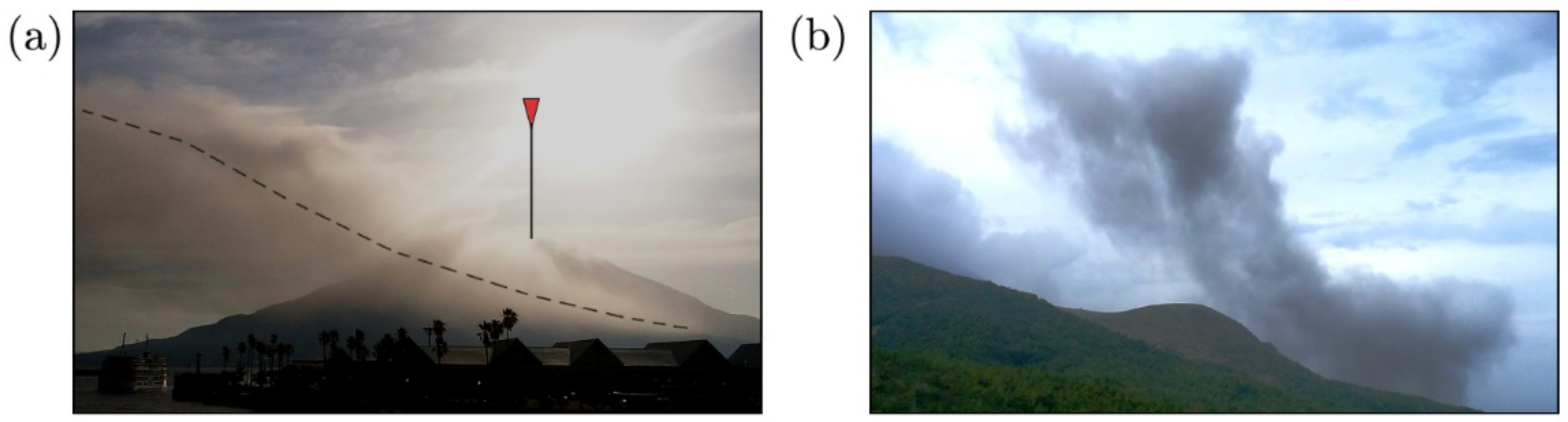
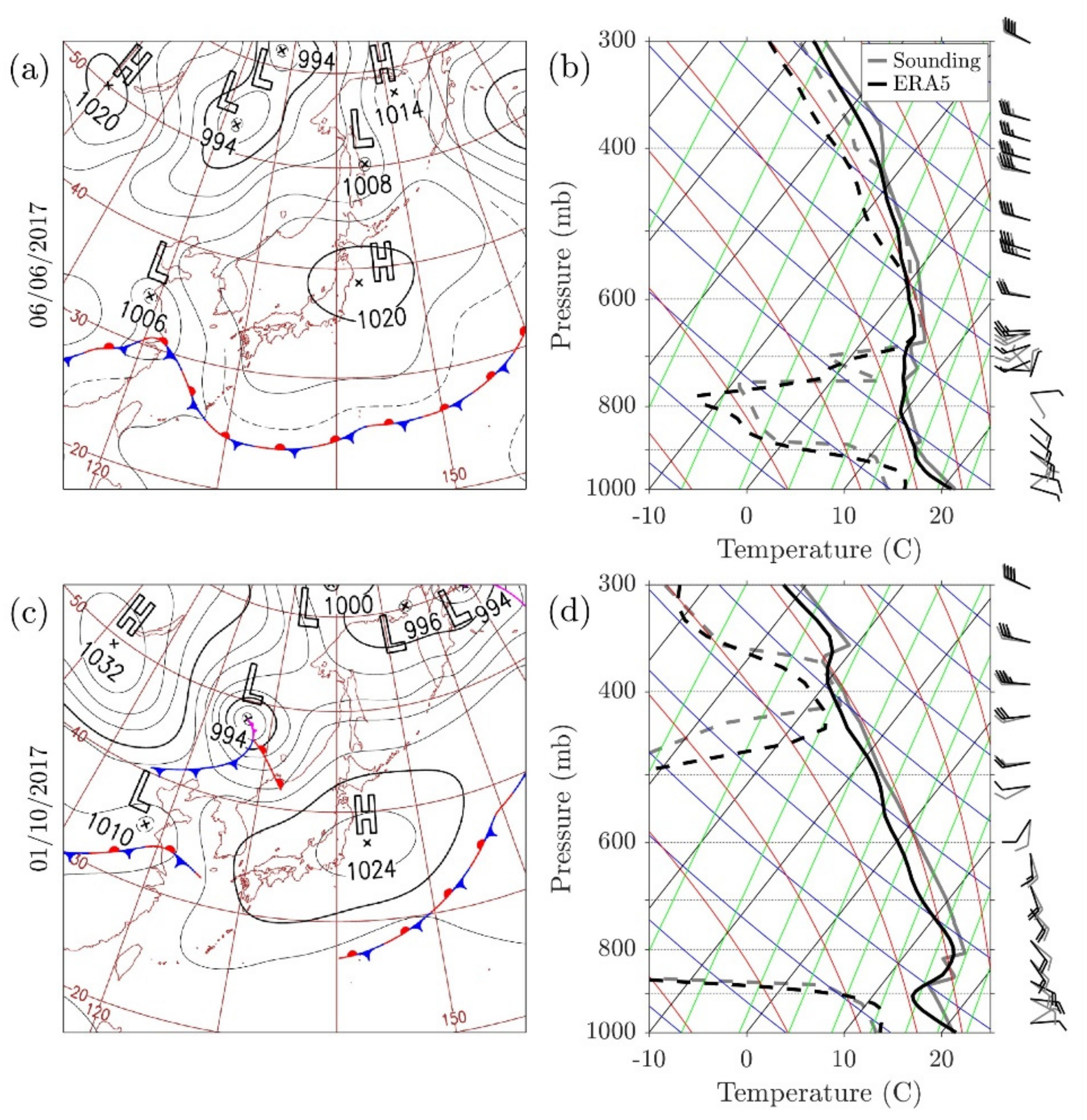
2. General Description of Case Study Days

The study focuses on the early morning hours of two days marked with volcanic eruptions: 6 June 2017 and 1 October 2017. The June eruption occurred at 0756 Japan Standard Time (JST; JST = UTC + 9 h), with a short initial phase (1–3 min; ash ejected over 3 km and concealed by cloud cover), followed by intermittent emissions a few hundred meters agl over the following hour. Ash from the initial phase was transported eastwards, while ash from the second phase was transported westwards, owing to the synoptic conditions (Figure 3a). On the day of the eruption, the Japan Meteorological Agency (JMA) reported that Kyushu entered the rainy season, a weather pattern dominated by the Baiu front; a stationary warm front south–southeast of the Japanese islands caused by the interaction of near–surface cool polar masses and warm tropical masses from the southwest. This is evident in the vertical structure of the atmosphere (Figure 3b). Close to the surface, wind direction is northeasterly, with the wind turning geostrophic at approximately 900 hPa. The two air masses are mixed between 800–700 hPa, leading to a layer of significant directional shear, which is capped with a temperature inversion and a cloud layer at 700 hPa. Above the inversion, wind direction is westerly, and the moisture content is increased.

The October eruption occurred at 0613 JST and lasted for $~1$ h, featuring a volcanic plume height of $~1$ km agl that was transported towards the west, with the effect of vertical wind shear apparent due to the significant fanning of the ash cloud (Figure 2a). The synoptic conditions were very similar to the June case, with circulation dictated by a combination of a high–pressure system to the east and a low–pressure system to the west (Figure 3c). Close to the surface observed wind directions were northeasterly, with the wind turning geostrophic at approximately 800 hPa, accompanied by a temperature inversion. Unlike the June case, wind direction was southerly with height, turning westerly above 600 hPa owing to the influence of the subtropical jet stream [45].

The vertical structure for both days is captured well in the European Reanalysis 5 (ERA5) [46] dataset (shown in black in Figure 3b,d). Despite the overall match between the ERA5 and sounding data, significant disagreement can be seen close to the surface (with the ERA5 data failing to reproduce the northeasterly surface flow) and below the change to the westerly flow ($~800$ hPa in Figure 3b and $~600$ hPa in Figure 3d). Other than wind direction, in the October case, the ERA5 data overestimate the temperature lapse rate close to the surface. For both days, the wind shear structure is consistent between 0400–0900JST. Up to 1 km above sea level (asl), the wind shear profile for both days is very similar, albeit with a $~15°$ difference (Figure 4). Differences between the two profiles are evident above 1 km asl as the sharp turn in wind direction is evident in the June case (Figure 4a) while in the October case, wind direction stays between 110–150$°$ (Figure 4b).

On both days, a Doppler lidar was placed on the west (lee with respect to low–level flow) side of the volcano (see Figure 1b and Section 3.1). For both cases, the perturbation part of vertical velocity (based on a 30 min moving average) revealed oscillations captured between $~100–300$ m agl (Figure 5). During the June case, these oscillations were mainly concentrated around a period ($T$) of 10 min (Figure 5a), while in the October case, the main peak in amplitude is associated $T=3$ min (Figure 5c). Waveforms presumed to be associated with gravity waves can be clearly seen in the signal (Figure 5b,d) after a moving average of $T/3$ (i.e., 3 and 1 min, respectively) has been applied. At an average advection speed 3.4 and 7 m s^–1 for the June and October cases, respectively, these values lead to a length scale of 2040 and 1260 m ($\approx O\left(1 \mathrm{km}\right)$), which are comparable to the volcano’s geometrical characteristics.

3. Methodology

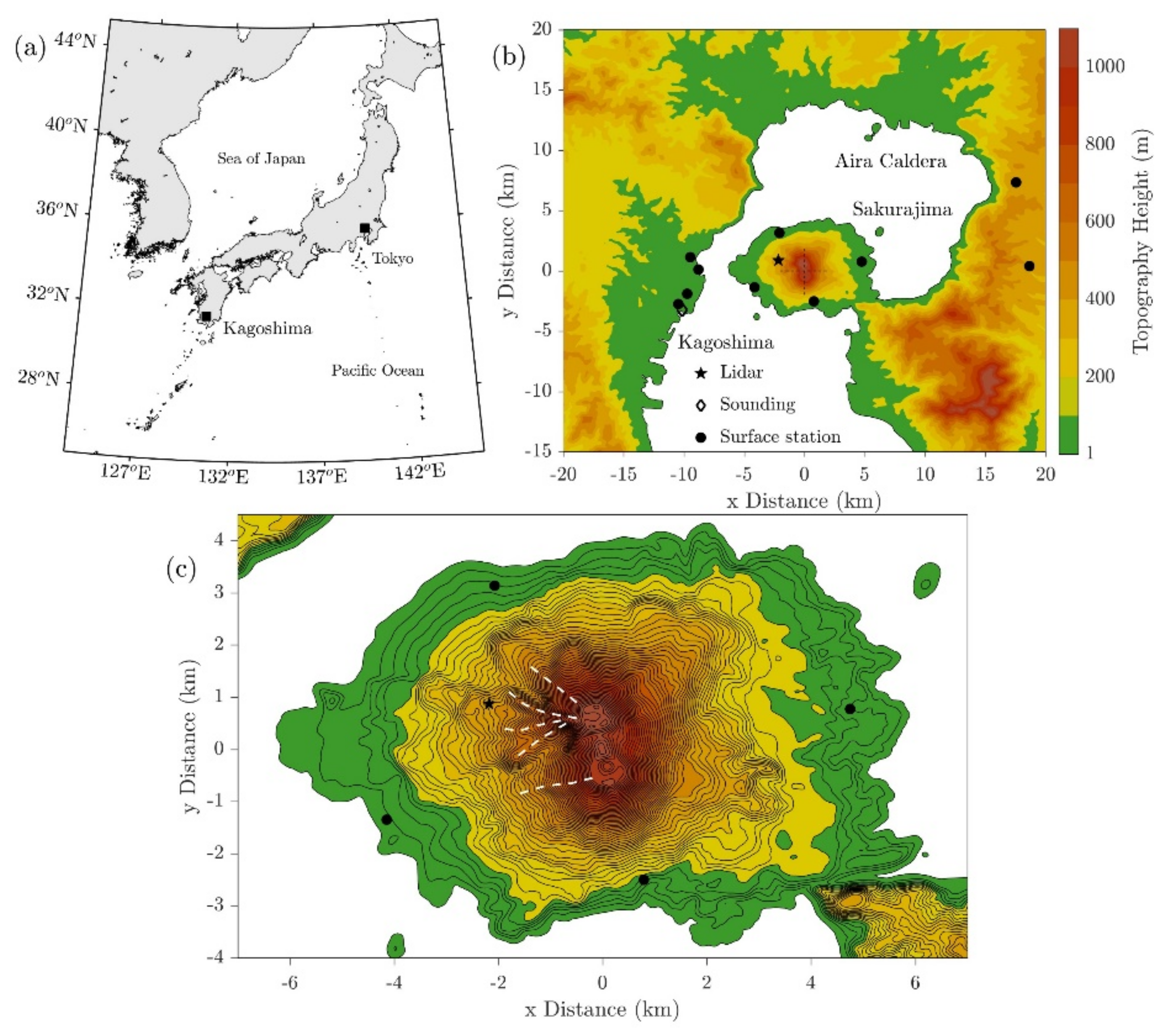
3.1. Observational Equipment

Acquisition of in–situ data over mountainous terrain is always a challenge [47] and volcanic activity further complicates the issue [48]. Owing to the long–lasting activity of the Sakurajima volcano (since 1955) and the health concerns for the residents in the vicinity [49], an automated observational network is operated near the volcano. In order to minimize ambiguity in the atmospheric state rawinsonde data, surface station and averaged Doppler lidar data were used to characterize the stationary response of the flow, while instantaneous Doppler lidar data are used to assess instantaneous winds and the magnitude of turbulence.

Surface wind speed and direction are measured by two nation–wide systems (circle markers in Figure 1b): seven stations from the Ministry of Environment’s (MoE) Atmospheric Environmental Regional Observation System (AEROS or Soramame in Japanese, http://soramame.taiki.go.jp/ (accessed date 25 February 2021); see [3] for details) and three stations from the Automated Meteorological Data Acquisition System (AMeDAS, https://www.jma.go.jp/jma/en/Activities/amedas/amedas.html (accessed date 25 February 2021)). All data are hourly, but AEROS data are instantaneous while AMeDAS data are 10–min averages of the values before the observation. For both systems, wind direction data are limited to 16 directions (i.e., have $\pm 11.25°$ error). Rawinsondes are launched twice daily from the meteorological station in the city of Kagoshima (31.55$°$ N/130.55$°$ E, World Meteorological Organization (WMO) code: 47827; diamond marker in Figure 1b) at 0900 and 2100JST.

Doppler lidars have been commonly used to measure wind speed and turbulence characteristics in a number of cases in mountainous terrain [50,51] and in harsh environments [52,53]. An optical–fiber Doppler lidar (LR–07F type III S; Mitsubishi Electric Corporation, Japan) is continuously operating on Sakurajima [54], located near the top of Mt. Haruta (31.59$°$ N/130.63$°$ E; star marker in Figure 1b). The wavelength is 1.5–1.6 $\mathsf{\mu }\mathrm{m}$, and the lidar is set pointing upwards, with a vertical resolution of 30 m between 30–600 m agl. Usable data usually lie within a thinner layer between 100–300 m agl ($~$500–700 m asl). The laser pulse width is 200 ns and the pulse repetition rate is 4 kHz. This leads to an effective frequency of $~$0.1667 Hz (i.e., $~$1 measurement per 6 s). Here, a 30–sec moving average was applied to remove noise from the data and values were then resampled to one observation per minute ($~$0.0167 Hz).

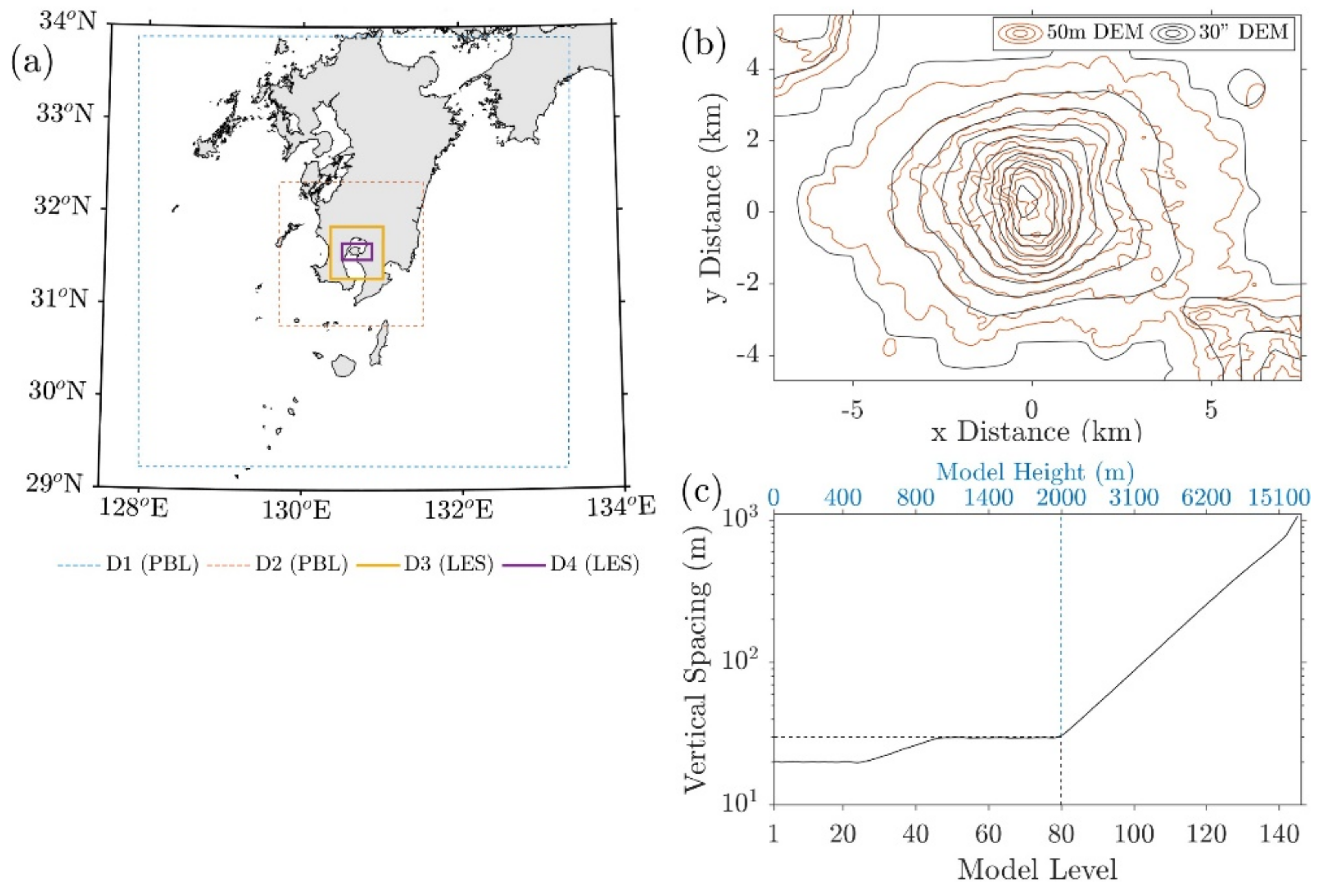
3.2. WRF Model Settings

Simulations were carried out using WRF version 4 [40]. As noted in Section 2, the dominant length scale for a stable PBL is unresolvable here. Instead, the horizontal grid spacings for the LES domains were chosen to represent gravity wave related instabilities, with dominant length scales of a few hundred meters [21]. Four one–way nested domains were used in total, progressively focusing over the volcano (Figure 6). For the two outermost domains, D1 and D2 (Figure 6a), with both 166 by 166 horizontal grid points at $\Delta x$ = 3150 and 1050 m, respectively, a PBL parametrization scheme [55] was utilized, while for the two innermost domains, D3 and D4 (Figure 6a), with 421 by 421 horizontal grid points at $\Delta x$ = 150 and 721 by 394 horizontal grid points at $\Delta x$ = 50 m, respectively, an LES scheme [56] was used. No turbulence–seeding technique [34,39] was used, as turbulence seeded at the boundaries is expected to diminish with distance. The reason why one–way nesting is used is because the horizontal sizes of the inner domains are limited and, thus, any resolved features in the inner domains will be quickly wiped out by the incoming flows at the lateral boundaries or the effects of the feedback from an inner domain to its direct parent domain will be limited.

In the vertical, 147 levels were used for all domains (80 levels within the lowest 2 km, 50 hPa model top; Figure 6c). Vertical grid spacing increases from $~$20 to 30 m within the lower 2 km and up to 1 km near the model top (Figure 6c) A Rayleigh damping layer with an inverse time scale was used for the top 5 km to reduce errors from gravity waves reflected at the domain top [57], while sixth–order monotonic horizontal diffusion (coefficient value of 0.12) was applied to minimize spurious behavior at poorly resolved scales [58]. Other physical parametrization schemes used were the RRTMG scheme [59] for radiative transfer, the MM5 surface layer scheme [60], and the Noah land surface model [61].

For all simulations, the topography was based on the Geospatial Information Authority of Japan (GSI) 50 m digital elevation model (DEM). Simulations were carried out using the model’s default terrain following coordinates, with a minimal amount of smoothing to ensure numerical stability over steep slopes. Even after smoothing, the DEM is able to represent the topographical features, such as the ridges of the west side of the volcano, well (Figure 6b; orange lines). As complex terrain is usually the reason for computational instabilities, which necessitate small time steps, a sensitivity simulation was also carried out for the June case using the default Global 30″ elevation (GTOPO30) DEM (Figure 6b; gray lines). After this sensitivity run, we have set the time step for D4.

Because of the complex features of the model topography generated by the high–resolution DEM data, the time steps of the temporal integration from D1 to D4 are set to 18, 6, 0.1, and 0.033 s, respectively.

The simulations were initialized using the ERA5 reanalysis data ($\Delta x~$31 km, 137 vertical levels). The outermost domain boundaries were specified using ERA5 hourly data. The simulations for the PBL domains for both cases started at 1200 UTC (2100 JST) of the previous day and were run for a total of 12 h to allow for the model spin–up. Simulations for the LES domains were initialized a later point to minimize computational time: six hours in the simulation for D3 (three hours of spin–up time) and eight hours for D4 (1 h spin–up time to allow for the main flow to travel from the lateral boundaries past the main study area). Data were output every minute.

3.3. Particle Trajectory Modeling

In order to quantify the magnitude of the impact the detailed airflow over the complex volcanic terrain has on the fall speed of particles near the volcano, idealized particle fall calculations were carried out over the 3 h average wind fields (0600–0900JST). Initially, 100 particles were randomly introduced in the domain using an ellipsoid distribution.

Idealized particles trajectories were calculated here. Calculations were carried out for two vertical velocity fields: (i) $W_0=-U_T$, where $-U_T$ is the terminal velocity of the particle, representing the case of particles falling unperturbed, and (ii) $W_{Pert}=\overline{w}-U_T$, where $\overline{w}$ (the WRF vertical velocity output) was added to represent the influence of detailed topography. In both cases, calculations were carried out using the model output for the horizontal wind fields. Five terminal velocities were chosen: 8, 4, 2, 1, and 0.3 m s^–1, to represent typical sizes and types of ash particles based on the formula [5], corresponding to 1, 0.5, 0.25, 0.125, and 0.063 mm for single particles (density ρ_A = 2500 kg m^–3) and 2, 1, 0.5, 0.25, and 0.125 mm for an aggregate (ρ_A = 750 kg m^–3).

It is noted that the effects of heating of the atmosphere from volcanic eruption are not incorporated in the present trajectory modeling. How to formulate the effects of heating due to volcanic eruption in the trajectory modeling will be an interesting topic; however, this study does not take into account this heating effect, because the central focus here is placed on the influences of the complex topography on airflows and particle transport and sedimentation.

4. Results

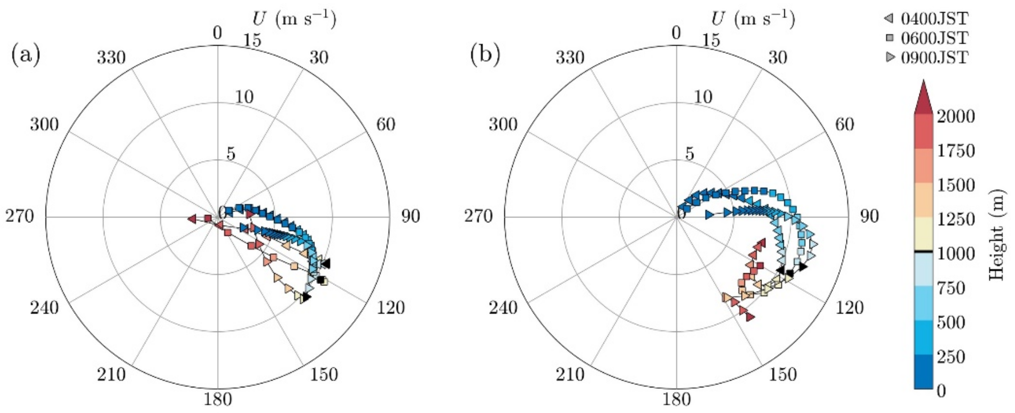
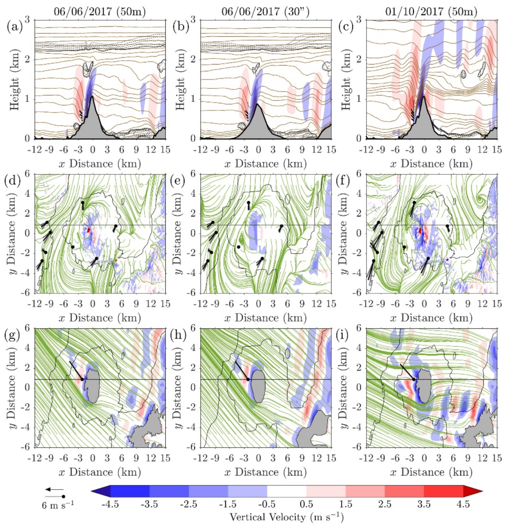
4.1. Stationary Flow Characteristics

Output from the innermost WRF model domain (D4) is shown as 3–h averages in Figure 7. In the June simulations (Figure 7a,b) flow is from the east (i.e., right side) up until the flow reversal point at 2 km. Mountain waves are triggered over the ridge to the east of the domain and in the lee side of the volcano, but are damped with distance due to the effect of the boundary layer acting as a sponge layer [62]. The location of the upwards component of the wave on the volcano lee matches the lidar observations (shown as black wind vectors). Gravity wave activity is also completely damped above the flow reversal point. A layer of flow reversal can be seen between the eastern ridge and the volcano up to 250 m from the surface, and a lee–side vortex can be seen immediately to the lee of the volcano. Finally, two isolated areas of flow reversal can be seen between the gravity waves and the westerly flow layer, from 1.6–2 km. Simulations using different DEMs are qualitatively similar.

Gravity wave activity is also dominant in the October simulation (Figure 7c). Over the eastern ridge, gravity waves are triggered over the inversion layer, with two rotors forming between the waves and the inversion (seen as areas of flow reversal). Over the volcano, the flow response is a hydraulic jump. Lidar observations match with the position of the upwards component of the wave and show an increased magnitude over the June case.

The wind direction shear and multiple topographic maxima combination leads to a complicated surface flow for both days, as visualized by streamlines. Despite significant differences in the vertical structure above $~$1 km, common elements can be seen for both case study days (Figure 7d–f). Inside the Aira caldera, the general flow is to the southwest, interrupted by the volcano causing flow divergence. A stagnation point can be seen for both days in the west side of the volcano (at approximately $x=0$ km, $y=3$ km) and an extended area of lee–vortices can be identified in the south–western side of the volcano. In an idealized setting, flow stagnation points are expected to be along the same axis as the lee vortices, but this is not the case here, owing to the wind direction shear. As with the vertical cross–section, using a 30″ DEM results in a qualitatively similar flow (Figure 7d,e).

The resolved flow is also in agreement with most surface observations that show a northeasterly flow. The location of the lee vortex is captured well, as seen by the station in the southwest of the volcano, which has a very small wind speed reading. Subtle changes in the wind direction owing to flow splitting are seen, although in the June case flow stagnation is overestimated in the western side of the volcano ($~x=5$ km, $y=1$ km). The single worst–matching point is located over the southern part of Kagoshima ($~x=10$ km, $y=-2$ km), which recorded an almost constant southeasterly wind, in contrast to the northeasterly wind recorded by the other stations in the city.

At 600~m asl, the flow is less complicated, with southeasterly winds in the June simulations (Figure 7g,h) with a more pronounced easterly component in the October case (Figure 7i). Streamlines show significant diversion as the flow meets the volcano. On the lee side, the gap created by the diverted flow is filled with the downslope wind seen in Figure 7a–c. A comparison against the lidar data at this height shows that the average wind direction is captured well in the lee of the volcano.

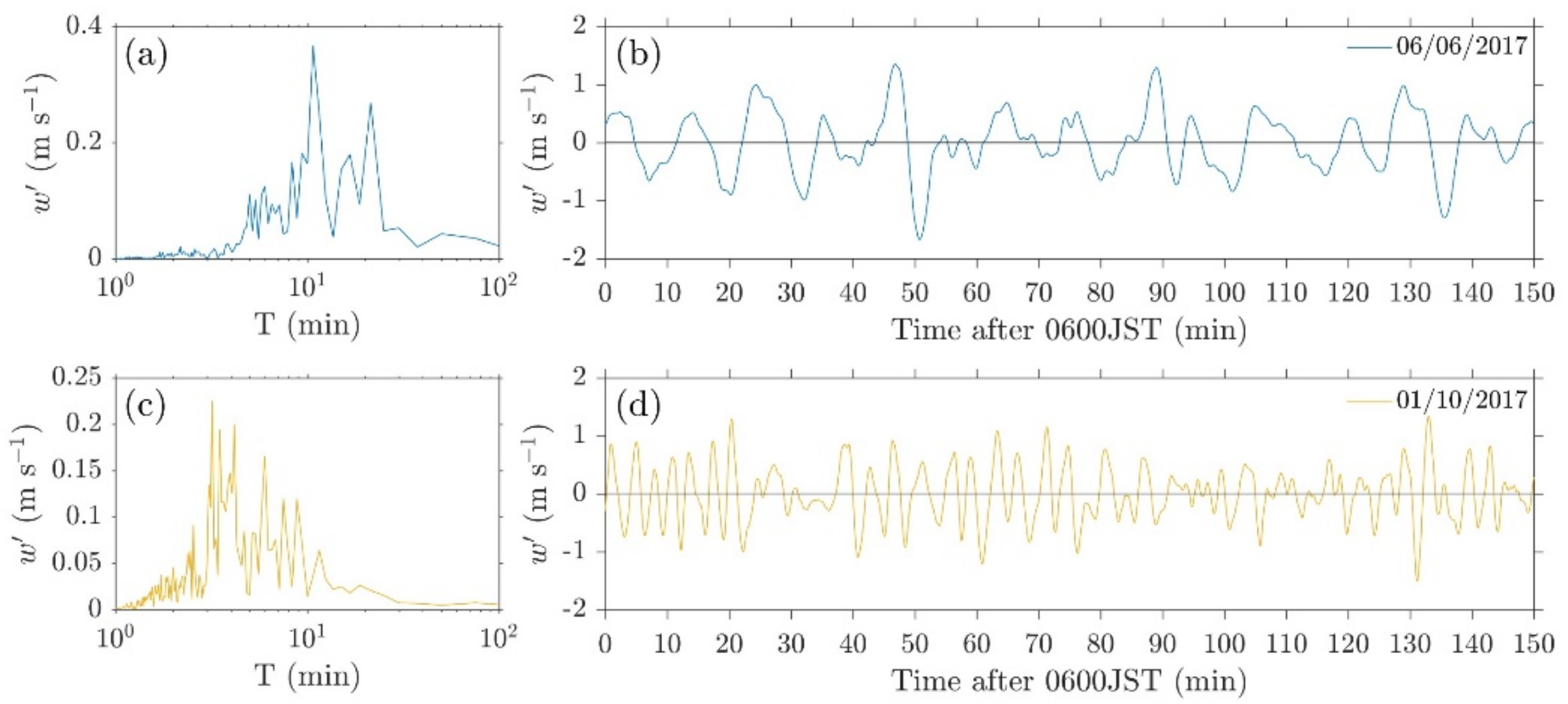
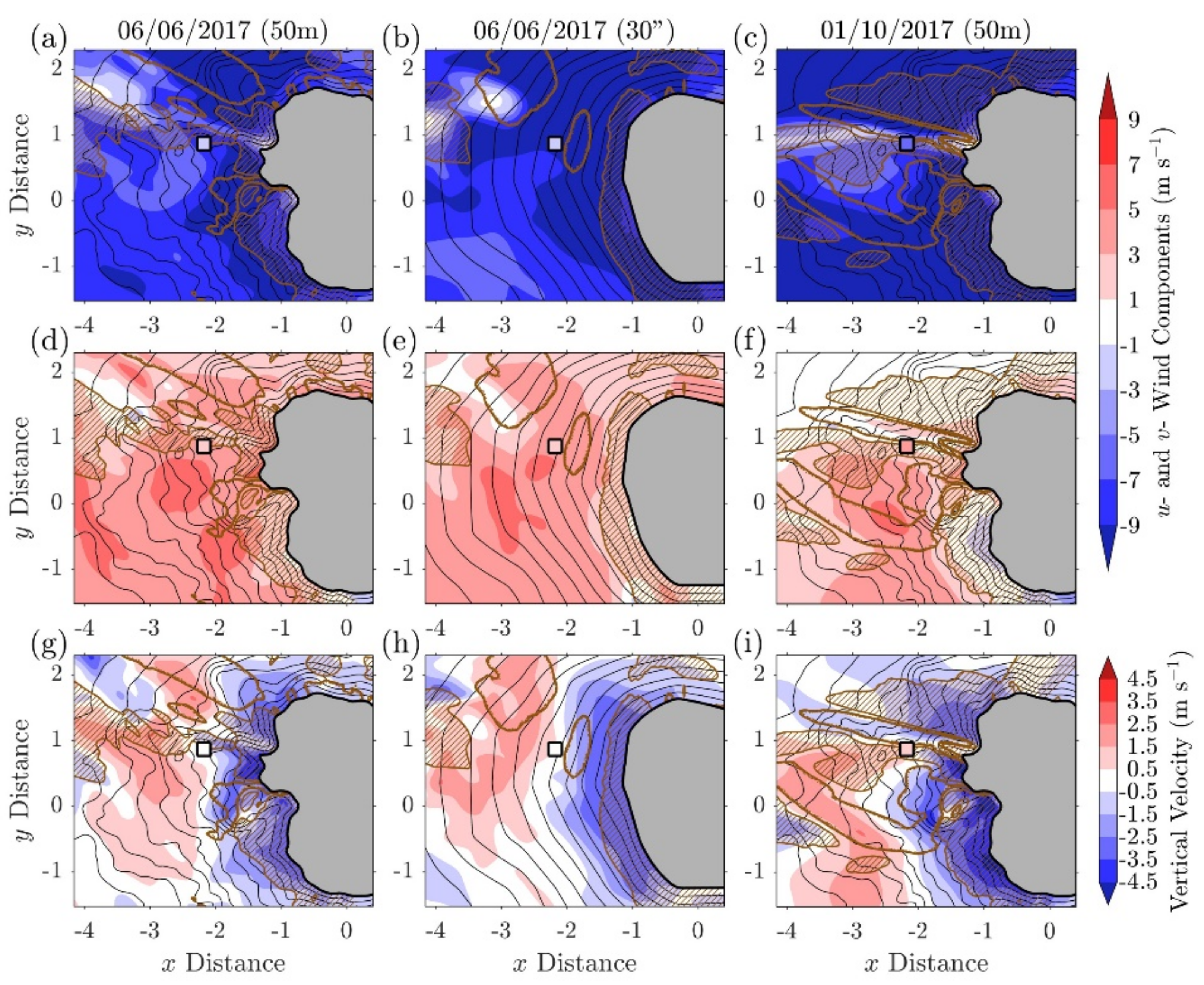
4.2. Lee–Side Turbulence Characteristics

The position of the Doppler lidar in the lee of the volcano provides an opportunity to compare the way mountain waves were modeled and the related turbulence characteristics. As the lidar was only able to consistently provide observations over a thin layer, results presented are averages between 500–700 m asl (centered at 600~m asl).

Figure 8 shows average values for the three wind components around the lidar side between 0600–0830 JST. Areas of significant absolute vorticity are also shown. A narrow wake region can be identified in the area between changing signs of absolute vorticity.

The wake region can also be identified as a local minimum in the $u$ component. In the case of the two 50 m DEM simulations (Figure 8a,c), the wake is generated by the lee–side ridges via a streak: vorticity is generated over the ridge as small changes in the wind direction lead to a downslope flow to either the left or the right side of the ridge. In the 30″ DEM simulations, the wake region is isolated (Figure 8b) and vorticity is generated due to the flow around the volcano (e.g., as in [63]). In the case of the June simulations, a series of weak vortices can be seen as changes between positive and negative values of both the $v$ and $w$ components (Figure 8d,g). The resolved wave pattern as seen through the averaged vertical velocity values (Figure 8g–i) closely mirrors the shape of the topography depending on the incident angle.

In the June (50 m DEM) simulation, a strict comparison against the lidar observations shows an overestimation of the $u$ and $v$ components (Figure 8a,d) and a correct representation of the $w$ component (Figure 8g). On the other hand, most values are represented appropriately in the October case, with only a small underestimation of the $v$ component (Figure 8f). In the case of less intricate topography (e.g., the volcano in the 30″ DEM simulation), the lee side patterns of all wind components are considerably smoother (and provide a worse match between lidar observations). As such, considering the proximity of the lidar location to the lee–side ridges and their connection to the low velocity streaks, it can be assumed that such errors in the spatial representation are tied to the complexity of the terrain and are inevitable to a certain degree.

The wake region is also associated with increased resolved turbulence kinetic energy ($k$) and low–period (high–frequency) oscillations in the vertical (Figure 9). Specifically, maxima in the $k$ distribution can be identified along areas of absolute vorticity sign change (Figure 9a–c). In the two 50 m DEM simulations, the area of increased $k$ intersects the volcano, while in the 30″ case it is disconnected from the topography. The June simulations show extended areas of $k>0.4$ m² s^–2, while in the October case, high $k$ values are only resolved across a narrow area in the lee of the volcano. Turbulence kinetic energy calculated based on the Doppler lidar measurements was 1.6 m² s^–2 for the June case and 2.3 m² s^–2 for the October case. The maximum resolved $k$ in the model in both 50 m DEM cases is 1.5 m² s^–2, showing that a significant part of the observed wave–related turbulence was resolved. In the October case, the area of increased $k$ overlaps with the Doppler lidar site; however, in the June case, the maximum values are located $~1$ km away from the site. This mirrors the spatial error seen in Figure 8.

Oscillations in the perturbation part of the vertical velocity component are dominated by high–period (low–frequency) areas (Figure 9d–f). However, areas of increased $k$ tend to be associated with low–period oscillations, similar to those seen in the Doppler lidar signal (Figure 8). In the June simulations, areas of low period can be identified scattered across the volcano lee–side, while in the October case, they closely mirror the area of increased $k$. In both cases, observed maxima in the $w^{\prime }$ distribution (10 and 3 min for the June and October cases, respectively) are resolved in the model, over (October) or near (June, 50 m) the Doppler lidar site.

As discussed in previous studies [64,65,66], the effects of turbulence on flow and dispersion are important in high–resolution simulations. In the present study, we intend to reproduce flow fluctuations generated by complex topography with the use of high–resolution DEM data. From the results shown in Figure 9, we are able to capture the turbulent flows observed by Doppler lidar in a certain degree. Because this study does not employ turbulence generation method at the lateral boundaries like those used in a turbulence recycling approach [34], fully turbulent flows such as seen in flows over rough surfaces would not develop. Complete LES modeling with a proper turbulent generation method at the lateral boundaries may be necessary to represent fully turbulent flows.

4.3. Sensitivity to Resolution

The WRF model is able to reproduce the vertical structure of the atmosphere reasonably well, as seen by a comparison against atmospheric sounding observations (Figure 10). The associated root mean square errors (RMSE) for all domains are small and generally decrease with an increase in resolution. At the innermost domain, the final RMSE values for wind speed and direction range between 1.2–2.4 m s^–1 and 11–13$°,$ respectively (Figure 10a,b). Although the error in wind direction decreases with increased resolution for the October case, this is not true for the June case, where RMSE values oscillate from 11–13$°$. WRF output also shows significant improvement in the representation of dynamic stability (shown by Richardson number, Ri; Figure 10c). In the June case, increased resolution leads to a small decrease in fidelity in relative humidity (1% increase over the outermost domains). Comparing the two June simulations shows a very small decrease in fidelity when using the 30″ DEM (star markers). Note that calculations were carried out from 0–10 km and as averages over a 31 km area at a single time (0900JST).

A comparison between average wind speed and wind direction values for each domain is also shown in detail in Figure 11. Increase in wind speed fidelity with increased resolution is mainly caused by the better representation of very low wind speed values, i.e., less than 2.5 m s^–1 (Figure 11a–d). In the June case, as most of the wind speed observations are small and as such resolved better in the innermost domain. On the other hand, the October case features a wider range of wind speed values, between 1–5 m s^–1. Increased model resolution in this case leads to a better match over the lower end of the range but underestimation at some points in the higher end (i.e., between 2.5–5 m s^–1).

Changes in wind direction do not exhibit a similar systematic improvement (Figure 10e–h). In all cases, wind direction away from the volcano is associated with small errors, while the stations over the volcano present a more significant challenge, especially in the June case that features overall lower wind speeds. As the surface flow has the largest amount of parameterized turbulence, results here point towards the existence of a minimum error with the current modeling approach.

Note that RMSE values shown for the AEROS stations (i.e., the instantaneous value output stations) are the minimum RMSE for that point in the domain at the time of the observations $\pm 7$ min. The time window was chosen to allow for a fair representation of the inherent turbulence that is included in the observations and was decided as the average time period for which the distribution of the perturbation part of the horizontal wind component differed less than 10% when compared to a 1 h average (i.e., the minimum time required to get a representative sample of randomness in the model output).

The resolved $w$ extrema (i.e., maximum and minimum) in the lee of the volcano ($x=\left[-4, -1\right]$ km, $y=\left[-1,2\right]$ km in e.g., Figure 8) for each domain are shown in Figure 12. At $\Delta x=~$3–1 km, D1 and D2 represent the high–end of common VATD resolutions. A small obstacle like Sakurajima is underestimated ($H_{max}=192$ and 602 m for D1 and D2, respectively), leading to maximum $w$ values of $O\left(0.1 {\mathrm{m}\mathrm{s}}^{-1}\right)$ for D1 and $O\left(1 {\mathrm{m}\mathrm{s}}^{-1}\right)$ for D2—negligible compared to the horizontal wind speed. However, the range increases considerably with increased resolution, up to $O\left(10 {\mathrm{m}\mathrm{s}}^{-1}\right)$ in the innermost domain, showing that in cases of such complex topography, the vertical velocity component can locally dominate the flow. Furthermore, these values are comparable to terminal velocities even for large particles. Simulations using the 30″ DEM (Figure 12b) show a significantly smaller range of vertical velocity values, showing that resolving the actual topography plays a vital role in the formation of the gravity wave response. Despite the increase in horizontal wind speed between the June and October cases, the resolved vertical velocity range is similar in both cases, although in the October simulation the extrema of the 3–h average are closer to the extrema based on the instantaneous values (Figure 12c).

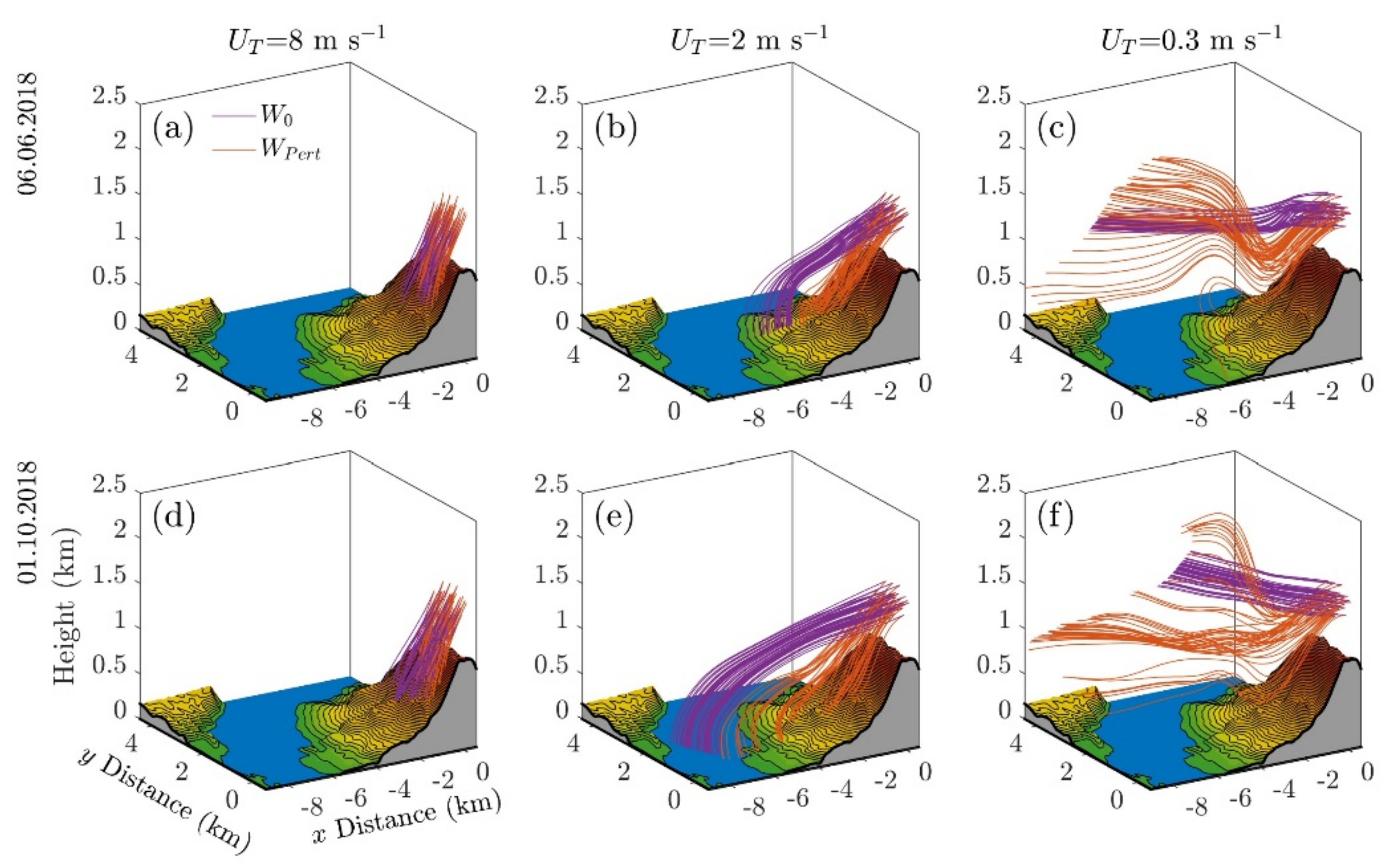
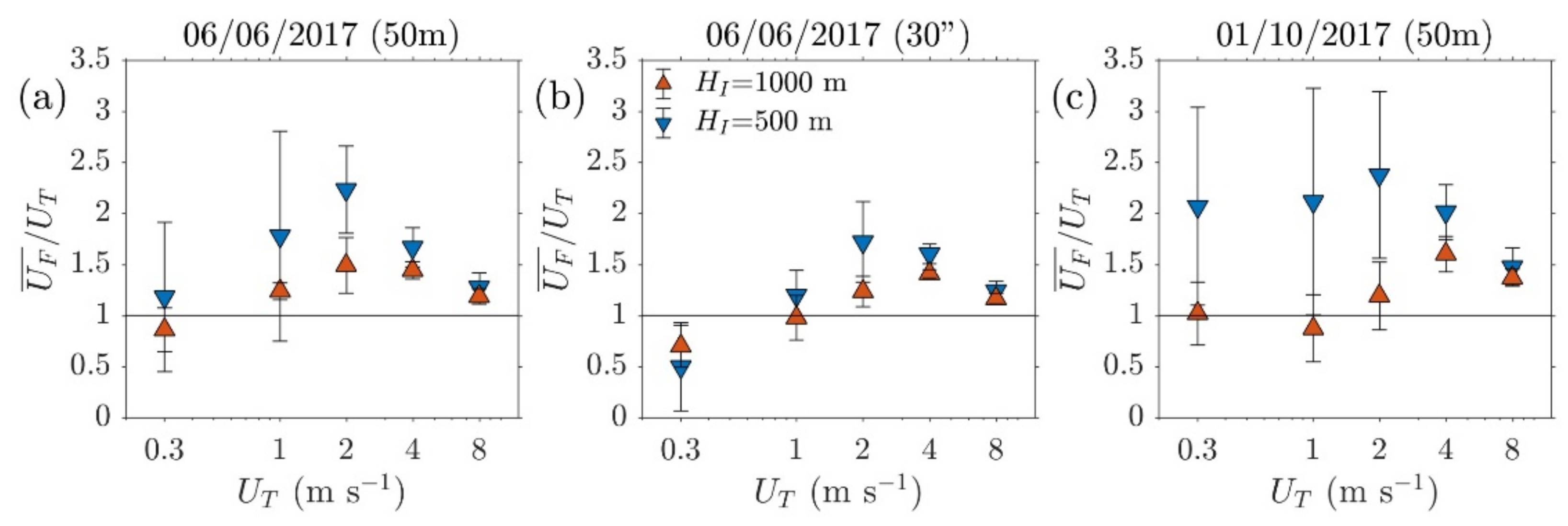
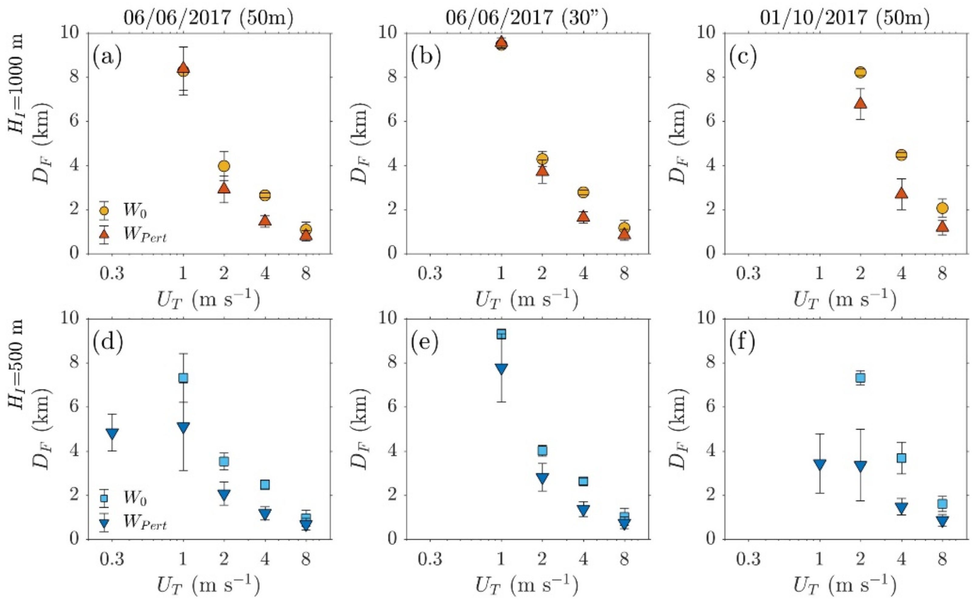
4.4. Particle Fall Trajectory Analysis

Overall, considering the complexity of the topography and vertical structure the model performs well even at coarse resolutions. Results show a consistent increase in fidelity and the range of $w$ was shown to significantly increase for the innermost domain. Although a comparison with Doppler lidar measurements revealed spatial inconsistencies, the resolved values were seen to be realistic for all three wind components. As such, results from D4 are used here to provide a basis for the idealized particle fall trajectory calculations of small to large particles ($U_T=$ 0.3, 1, 2, 4, and 8 m s^–1). As a first step, 3–h average wind field values are used to provide an order of magnitude evaluation. More precise calculations necessitate the use of a specialized transport model, further complicating the study. As such, simulating ash dispersal for the events will be the point of a future effort.

Example trajectories for the $W_0$ (no vertical velocity component) and $W_{Pert}$ (WRF vertical velocity added) are shown for an injection height of 500 m and three particle categories in Figure 13. In all cases, including the vertical velocity component leads to visibly different trajectories. In the $W_{Pert}$ calculations, large particles ($U_T=8$ and 2 m s^–1; Figure 13a,b,d,e) are captured by the downslope wind, which holds the trajectories close to the volcano’s slope (as seen in Figure 2b) and enforces deposition closer to the release location. In the intermediate case ($U_T=2$ m s^–1; Figure 13b,e), inclusion of the vertical velocity component leads to markedly different trajectories, with the deposition of particles occurring over the entire lee side of the volcano. The effect of the wind shear is also visible in all calculations, in a similar manner to Figure 2a. Finally, in the case of small particles, gravity wave activity mainly results in the vertical displacement of particle trajectories. Between the two days (first and second rows in Figure 13), results are similar; however, the differences between the $W_0$ and $W_{Pert}$ calculations are emphasized in the October case due to the larger horizontal wind component.

The impact of the gravity waves on the fall speed is shown via the ratio between the average fall speed to the terminal velocity (i.e., the unperturbed fall velocity), with values away from 1 showing a large deviation (Figure 14). In this sense, the impact is most notable for intermediate particles ($U_T=$ 1–4 m s–1; medium–sized ash particles). A comparison between the June and October simulations (Figure 14a,c) shows that the effect is emphasized in the case of more energetic flow conditions (i.e., the October case), while a comparison between the 50 m and 30″ DEM simulations (Figure 14a,b) shows that the smoother flow simulated using the 30″ DEM leads to a decreased impact on the fall speed. Finally, the injection height of the particles can also have a direct impact: in all cases, injecting particles at a 1000 m agl leads to ratios closer to 1.

A secondary characteristic is the range exhibited due to the random nature of the particle placement, which increases significantly for smaller terminal velocities (i.e., smaller particle sizes). Specifically in the case of $U_T$ in the June simulation (Figure 14a), although the ratio is close to 1, the standard deviation shows ratios constrained within a factor of 2, with values less than 1 showing particles that fall slower than their terminal velocity. This is due to the vertical displacement of the particle trajectories that was previously seen when discussing Figure 13c,f.

Finally, the impact of detailed airflow can be seen as a change in the deposition distance of the particles (Figure 15). As the perturbed fall velocities are, on average, higher than the terminal velocities, the deposition distance is generally smaller in the case of the $W_{Pert}$ calculations. For an injection height of 1000 m (Figure 15a–c), the effect on the distance is O(100 m) in the case of large ($U_T=8$ m s^–1) or small ($U_T=1$ m s^–1) particles, and O(1 km) for the intermediate sizes ($U_T=1, 2$ m s^–1), with the effect being more significant in the October case. Terminal velocity bins with no corresponding values indicate particles that did not get deposited within 10 km of the injection point.

In the case of an injection height of 500 m (Figure 15d–f), the difference in deposition distance becomes more pronounced for lighter particles, i.e., $U_T<2$ m s^–1, with a maximum difference of 3 km in the June case ($U_T=1$ m s^–1) and up to 4 km in the October case ($U_T=2$ m s^–1). Furthermore, in both June and October cases, 2–9% of the particles were forcedly deposited due to downslope winds; at $U_T=0.3$ m s^–1 for the June case and $U_T=1$ m s^–1 for the October case. In both cases, the average deposition distance is similar to that of the immediately larger particle size category (i.e., 0.3, 1 m s^–1 for the June case and 1, 2 m s^–1 for the October case).

5. Discussion and Conclusions

The WRF model was used in a multi–scale setting in order to conduct high–resolution simulations for two cases with a similar, complex vertical structure in the atmosphere. The Sakurajima volcano, Japan, was used as the study location due to the observational network around it and the need of detailed simulation data in order to understand the dynamics of transport of pollutants from the volcano. Four domains were used, with the outer domain initialized ERA5 reanalysis data. The two outermost domains employed a PBL parameterization, while the innermost two employed an LES scheme. The atmospheric motions resolved were seen to have two major components, a quasi–steady state response dominated by gravity waves, overlaid with localized turbulent perturbations in the wake regions of the various topographic maxima.

The overall steady–state flow pattern was resolved well in all domains, agreeing both with theoretical expectations (e.g., flow splitting, mountain wave generation, lee–side wake) as well as surface, near–surface, and synoptic data. Although the majority of surface wind observations were represented well in the model, misrepresentation of wind direction was also seen over some of the observation locations. In the most severe cases, a 120–140$°$ error in wind direction persisted even at the innermost domain. Misrepresentation of surface values of wind direction is a known issue with WRF: it was shown [67] that, especially in the case of complex topography, the associated error of wind direction correlates with wind speed—low wind speeds leading to large wind direction errors, which was also partially true for simulations shown here. Results here show that issues raised for simulations over coarser resolutions can be maintained even after the resolution allows for a faithful representation of the topography, highlighting limitations of the approach used.

Turbulent fluctuations were studied in detail for the lee–side of the volcano and it was seen that a realistic orographic flow response was resolved in the innermost (LES) domains. On average, the model was able to reproduce the observed characteristics of the flow response, both at the surface (flow splitting and surface rotors) and aloft (wake region). A comparison against Doppler lidar observations showed that a qualitative match was generally achieved in the simulations (i.e., location and magnitude of the various orographic phenomena); however, issues were noted concerning the spatial fidelity of the representation. The complexity in the topography of the western side of the volcano (lee–side in the cases studied here) is suspected to be a main cause of the mismatch.

Turbulence aloft was increased over a wake region and tied with gravity waves (a well–known connection); via changes in the absolute vorticity of the flow [68,69]. Turbulence generation was seen to occur as a combination of the large–scale flow around the volcano (resolved both in simulations using the detailed 50 m DEM as well as the smooth topography of the 30″ DEM), overlaid with a region of increased turbulence caused by the small–scale changes in the flow over the ridges on the lee–side of the volcano (resolved on when using the 50 m DEM). Due to the sensitivity of the orographic response to small changes in the wind speed and wind direction [70], it is assumed that over highly complex topography, a perfect spatial match would be difficult to achieve without data assimilation. Simulations using the 30″ DEM were shown to produce a smoother response on the lee–side. As such, it can be assumed that a spatial match might be more easily achievable in simulations over a location with smoother topography.

Results from the 30″ DEM simulation, although qualitatively very similar to those of the high–resolution (50 m) DEM, showed that the correct representation of topography can have a large impact on fidelity. Simulations using the 50 m DEM showed a consistent increase in fidelity in the representation of surface wind direction (by 6.5$°$), using the 30″ DEM led to a deteriorating match, with an increase in the associated error for wind direction (by 10.7$°$). Smoothing techniques are often employed in computational modeling over complex terrain, but results here show that taken to a relative extreme (as in the case presented here) smoothing can have a deteriorating effect on the output of high–resolution simulations. Similar results were noted in a model inter–comparison study [71], which studied rainfall and wind patterns over Kyushu in typhoon conditions and concluded that the way topography is resolved in the models had a significant effect in the results. The importance of using high–resolution DEM data in high–resolution atmospheric simulations was also emphasized in a heavy rainfall case [72] and in a strong wind case [73].

The proper representation of the detailed airflow is known to play a vital role in the proper simulations of pollutant transport [18,45,73,74]. Under stable conditions (common for Sakurajima volcano; [45]) and for particles that are either introduced close to the surface or, in the case of large eruptions, have fallen from a large height and are captured by orographic flows generated by distal mountains (for example as in the case discussed in [75]), the impact of localized airflows was noticeable even for heavy particles ($~20$% change in speed and up to 1 km difference in deposition distance). For particles that were not directly deposited, gravity wave activity was shown to force vertical displacement. As expected, the impact was seen to lessen with an increased injection height and can be expected to be negligible for particle transport a few kilometers above the surface. The calculation of particle settling velocity is a critical process in VATD models [12] and results here illustrate that modifying the calculated velocity over topographic maxima would be an easily implementable approach to parameterize the impact of orographic effects and improve accuracy both in VATD models, as well as backward trajectory calculations that are often performed on the field [75].

The main reason why this study used of an off–line model in the trajectory calculations is that in a volcanology viewpoint we would like to conduct a large number of sensitivity tests and follow a probabilistic approach due to uncertainties in the eruption source conditions. A fully coupled atmosphere–chemistry–aerosol model such as the WRF–chem performs favorably for a single deterministic simulation (and as emissions are handled internally it makes full use of WRF calculations on subgrid effects), but repeating the meteorological calculations after that can be significantly expensive in most volcanological settings (especially in the case of LES). Thus, the present off–line modeling framework should be useful in examining possible flow and dispersion patterns with some assumed eruptions conditions.

Overall, results further highlight the difficulties of accurately simulating volcanic ash deposition in the proximal region. Even using the modeling presented here, spatial fidelity was shown to be limited within a factor of O(100 m) due to the sensitivity of the resulting orographic effects on the inherent errors in the initialization data [70] as well as due to unresolved turbulence. In the case of VATD modeling, meteorological data are used along with estimated eruption source parameters (e.g., erupted mass, volcanic plume height, duration, ejected particle grain size) in order to estimate both the plume characteristics (e.g., shape, radius [76], as well as the transport of volcanic ash [77]). This leads to such applications being especially sensitive to systematic errors in the meteorological data as it affects both the initial condition (i.e., plume shape) as well as the transport. In order to counteract this effect in cases of high–resolution secondary modeling applications, an ensemble method could be used with slightly different initialization times to account for the randomness in the turbulence, or in cases where this is inapplicable, an empirical increase in horizontal and vertical diffusion. Recognizing these issues will contribute to deepen the understanding of atmospheric transport of volcanic ash with the use of a fully coupled atmosphere–chemistry–aerosol model such as the WRF–chem modeling system [18,78].

References

1. Steyn, D.G.; De Wekker, S.F.J.; Kossman, M.; Martilli, A. Boundary layers and air quality in mountainous terrain. In Mountain Weather Research and Forecasting; Springer: New York, NY, USA, 2013; pp. 261–289. [Google Scholar]
2. Cece, R.; Bernard, D.; Brioude, J.; Zahibo, N. Microscale anthropogenic pollution modelling in a small tropical island during weak trade winds: Lagrangian particle dispersion simulations using real nested LES meteorological fields. Atmos. Environ. 2016, 139, 98–112. [Google Scholar] [CrossRef]
3. Poulidis, A.P.; Takemi, T.; Shimizu, A.; Iguchi, M.; Jenkins, S.F. Statistical analysis of dispersal and deposition patterns of volcanic emissions from Mt. Sakurajima, Japan. Atmos. Environ. 2018, 179, 305–320. [Google Scholar] [CrossRef]
4. Vosper, S.; Ross, A.; Renfrew, I.; Sheridan, P.; Elvidge, A.; Grubisic, V. Current challenges in orographic flow dynamics: Turbulent exchange due to low–level gravity–wave processes. Atmosphere 2018, 9, 361. [Google Scholar] [CrossRef] [Green Version]
5. Bonadonna, C.; Ernst, G.G.J.; Sparks, R.S.J. Thickness variations and volume estimates of tephra fall deposits: The importance of particle Reynolds number. J. Volcanol. Geotherm. Res. 1998, 81, 173–187. [Google Scholar] [CrossRef]
6. Bonadonna, C.; Costa, A. Observational techniques: Sampling the mountain atmosphere. In Modeling Volcanic Processes: The Physics and Mathematics of Volcanism; Fagents, S.A., Gregg, T.K.P., Lopes, R.M.C., Eds.; Cambridge Academic Press: Cambridge, UK, 2013; pp. 173–202. [Google Scholar]
7. Manzella, L.; Bonadonna, C.; Phillips, J.C.; Monnard, H. The role of gravitational instabilities in deposition of volcanic ash. Geology 2015, 43, 211–214. [Google Scholar] [CrossRef] [Green Version]
8. Scollo, S.; Bonadonna, C.; Manzella, I. Settling–driven gravitational instabilities associated with volcanic clouds: New insights from experimental investigations. Bull. Volcanol. 2017, 79, 30. [Google Scholar] [CrossRef] [Green Version]
9. Smith, R.B. Linear theory of stratified hydrostatic flow past an isolated mountain. Tellus 1980, 32, 348–364. [Google Scholar] [CrossRef] [Green Version]
10. Durran, D.R. Mountain waves and downslope winds. In Atmospheric Processes Over Complex Terrain; Meteorological Monographs; American Meteorological Society: Boston, MA, USA, 1990; pp. 59–81. [Google Scholar]
11. Armienti, P.; Macedonio, G.; Pareschi, M.T. A numerical model for simulation of tephra transport and deposition: Applications to May 18, 1980, Mount St. Helens eruption. J. Geophys. Res. 1988, 93, 6463–6476. [Google Scholar] [CrossRef]
12. Folch, A. A review of tephra transport and dispersal models: Evolution, current status, and future perspectives. J. Volcanol. Geotherm. Res. 2012, 235, 96–115. [Google Scholar] [CrossRef]
13. Folch, A.; Jorba, O.; Viramonte, J. Volcanic ash forecast–application to the May 2008 Chaiten eruption. Nat. Hazards Earth Syst. Sci 2008, 8, 927–940. [Google Scholar] [CrossRef]
14. Corradini, S.; Merucci, L.; Folch, A. Volcanic ash cloud properties: Comparison between MODIS satellite retrievals and FALL3D transport model. IEEE Geosci. Remote Sens. 2011, 8, 248–252. [Google Scholar] [CrossRef]
15. Osores, M.S.; Folch, A.; Collini, E.; Villarosa, G.; Durant, A.; Pujol, G.; Viramonte, J.G. Validation of the FALL3D model for the 2008 Chaiten eruption using field and satellite data. Andean Geol. 2013, 40, 262–276. [Google Scholar] [CrossRef] [Green Version]
16. Steensen, T.; Stuefer, M.; Webley, P.; Grell, G.; Freitas, S. Qualitative comparison of Mount Redoubt 2009 volcanic clouds using the PUFF and WRF–Chem dispersion models and satellite remote sensing data. J. Volcanol. Geotherm. Res. 2013, 259, 235–247. [Google Scholar] [CrossRef]
17. Hasegawa, Y.; Sugai, A.; Hayashi, Y.; Hayashi, Y.; Saito, S.; Shimbori, T. Improvements of volcanic ash fall forecasts issued by the Japan Meteorological Agency. J. Appl. Volcanol. 2015, 4, 2. [Google Scholar] [CrossRef] [Green Version]
18. Poulidis, A.P.; Takemi, T.; Iguchi, M.; Renfrew, I.A. Orographic effects on the transport and deposition of volcanic ash: A case study of Mt. Sakurajima, Japan. J. Geophys. Res. Atmos. 2017, 122, 9332–9350. [Google Scholar] [CrossRef]
19. Poulidis, A.P.; Phillips, J.C.; Renfrew, I.A.; Barclay, J.; Hogg, A.; Jenkins, S.F.; Robertson, R.; Pyle, D.M. Meteorological controls on local and regional volcanic ash dispersal. Sci. Rep. 2018, 89, 6873. [Google Scholar] [CrossRef]
20. Wyngaard, J.C. Toward numerical modeling in the “terra incognita”. J. Atmos. Sci. 2004, 61, 1816–1826. [Google Scholar] [CrossRef]
21. Zhou, B.; Chow, F.K. Nested large–eddy simulations of the intermittently turbulent stable atmospheric boundary layer over real terrain. J. Atmos. Sci. 2014, 71, 1021–1039. [Google Scholar] [CrossRef]
22. Ching, J.; Rotunno, R.; Lemone, M.; Martilli, A.; Kosovic, B.; Jimenez, P.A.; Dudhia, J. Convectively induced secondary circulations in fine–grid mesoscale numerical weather prediction models. Mon. Weather Rev. 2014, 142, 3284–3302. [Google Scholar] [CrossRef]
23. Takemi, T.; Rotunno, R. The effects of subgrid model mixing and numerical filtering in simulations of mesoscale cloud systems. Mon. Weather Rev. 2003, 131, 2085–2101. [Google Scholar] [CrossRef]
24. Rai, R.K.; Berg, L.K.; Kosovic, B.; Mirocha, J.D.; Pekour, M.S.; Shaw, W.J. Comparison of measured and numerically simulated turbulence statistics in a convective boundary layer over complex terrain. Bound. Layer Meteorol. 2017, 163, 69–89. [Google Scholar] [CrossRef]
25. Sauer, J.A.; Munoz-Esparza, D.; Canfield, J.M.; Costigan, K.R.; Linn, R.R.; Kim, Y.-J. A large–eddy simulation study of atmospheric boundary layer influence on stratified flows over terrain. J. Atmos. Sci. 2016, 73, 2615–2632. [Google Scholar] [CrossRef]
26. Ma, Y.; Liu, H. Large–eddy simulations of atmospheric flows over complex terrain using the immersed–boundary method in the weather research and forecasting model. Bound. Layer Meteorol. 2017, 165, 421–445. [Google Scholar] [CrossRef]
27. Xie, Z.-T.; Castro, I.P. Large–eddy simulation for flow and dispersion in urban streets. Atmos. Environ. 2009, 43, 2174–2185. [Google Scholar] [CrossRef] [Green Version]
28. Lundquist, K.A.; Chow, F.K.; Lundquist, J.K. An immersed boundary method enabling large–eddy simulations of flow over complex terrain in the WRF model. Mon. Weather Rev. 2012, 140, 3936–3955. [Google Scholar] [CrossRef]
29. Yoshida, Y.; Takemi, T.; Horiguchi, M. Large–eddy–simulation study of the effects of building–height variability on turbulent flows over an actual urban area. Bound. Layer Meteorol. 2018, 168, 127–153. [Google Scholar] [CrossRef] [Green Version]
30. Takemi, T.; Yoshida, T.; Horiguchi, M.; Vandebauwhede, W. Large–eddy–simulation analysis of airflows and strong wind hazards in urban areas. Urban Clim. 2020, 32, 100625. [Google Scholar] [CrossRef]
31. Duan, G.; Takemi, T. Gustiness in thermally–stratified urban turbulent boundary–layer flows and the influence of surface roughness. J. Wind Eng. Ind. Aerodyn. 2021, 208. [Google Scholar] [CrossRef]
32. Nakayama, H.; Takemi, T.; Nagai, H. Large–eddy simulation of turbulent winds during the Fukushima Daiichi Nuclear Power Plant accident by coupling with a meso–scale meteorological simulation model. Adv. Sci. Res. 2015, 12, 127–133. [Google Scholar] [CrossRef] [Green Version]
33. Nakayama, H.; Takemi, T.; Nagai, H. Development of local–scale high–resolution atmospheric dispersion model using large–eddy simulation. Part 5: Detailed simulation of turbulent flows and plume dispersion in an actual urban area under real meteorological conditions. J. Nucl. Sci. Tech. 2016, 53, 887–908. [Google Scholar] [CrossRef]
34. Nakayama, H.; Takemi, T.; Nagai, H. Large–eddy simulation of urban boundary–layer flows by generating turbulent inflows from mesoscale meteorological simulations. Atmos. Sci. Lett. 2012, 13, 180–186. [Google Scholar] [CrossRef]
35. Neggers, R.A.J.; Siebesma, A.P.; Heus, T. Continuous single–column model evaluation at a permanent meteorological supersite. Bull. Amer. Meteor. Soc. 2012, 93, 1389–1400. [Google Scholar] [CrossRef] [Green Version]
36. Endo, S.; Fridlind, A.M.; Lin, W.; Vogelmann, A.M.; Toto, R.; Ackerman, A.S.; McFarquhar, G.M.; Jackson, R.C.; Jonsson, H.H.; Liu, Y. RACORO continental boundary layer cloud investigations: 2. Large–eddy simulations of cumulus clouds and evaluation with in situ and ground–based observations. J. Geophys. Res.—Atmospheres. 2015, 120, 5993–6014. [Google Scholar] [CrossRef] [Green Version]
37. Heinze, R.; Moseley, C.; Boske, C.M.; Muppa, S.; Maurer, V.; Raasch, S.; Stevens, B. Evaluation of large–eddy simulations forced with mesoscale model output for a multi–week period during a measurement campaign. Atmos. Chem. Phys. 2017, 17, 7083–7109. [Google Scholar] [CrossRef] [Green Version]
38. Talbot, C.; Bou–Zeid, E.; Smith, J. Nested mesoscale large–eddy simulations with WRF: Performance in real test cases. J. Hydrometeorol. 2012, 13, 1421–1441. [Google Scholar] [CrossRef]
39. Munoz–Esparza, D.; Kosovic, B.; Mirocha, J.; van Beeck, J. Bridging the transition from mesoscale to microscale turbulence in numerical weather prediction models. Bound. Layer Meteorol. 2014, 153, 409–440. [Google Scholar] [CrossRef]
40. Skamarock, W.C.; Klemp, J.B.; Dudhia, J.; Gill, D.O.; Liu, Z.; Berner, J.; Wang, W.; Powers, J.G.; Duda, M.G.; Barker, D.; et al. A Description of the Advanced Research WRF Model Version 4; NCAR/TN–556+STR: Boulder, CO, USA, 2019. [Google Scholar]
41. Chu, X.; Xue, L.; Geerts, B.; Rasmussen, R.; Breed, D. A case study of radar observations and WRF LES simulations of the impact of ground–based glaciogenic seeding on orographic clouds and precipitation. Part I: Observations and model validations. J. Appl. Meteorol. Clim. 2014, 53, 2264–2286. [Google Scholar] [CrossRef] [Green Version]
42. Nugent, A.D.; Watson, C.D.; Thompson, G.; Smith, R.B. Aerosol impacts on thermally driven orographic convection. J. Atmos. Sci. 2016, 73, 3115–3132. [Google Scholar] [CrossRef]
43. Xue, L.; Chu, X.; Rasmussen, R.; Breed, D.; Geerts, B. A case study of radar observations and WRF LES simulations of the impact of ground–based glaciogenic seeding on orographic clouds and precipitation. Part II: AgI dispersion and seeding signals simulated by WRF. J. Appl. Meteorol. Clim. 2016, 55, 445–646. [Google Scholar] [CrossRef]
44. Caccamo, M.T.; Castorina, G.; Colombo, F.; Insinga, V.; Maiorana, E.; Magazù, S. Weather forecast performances for complex orographic areas: Impact of different grid resolutions and of geographic data on heavy rainfall event simulations in Sicily. Atmos. Res. 2017, 198, 22–33. [Google Scholar] [CrossRef]
45. Poulidis, A.P.; Takemi, T. A 1998–2013 climatology of Kyushu, Japan: Seasonal variations of stability and rainfall. Int. J. Clim. 2017, 37, 1843–1858. [Google Scholar] [CrossRef] [Green Version]
46. Hersbach, H.; Bell, B.; Berrisford, P.; Hirahara, S.; Horányi, A.; Muñoz-Sabater, J.; Nicolas, J.; Peubey, C.; Radu, R.; Schepers, D.; et al. The ERA5 global reanalysis. Quart. J. Roy. Meteorol. Soc. 2020, 146, 1999–2049. [Google Scholar] [CrossRef]
47. Banta, R.B.; Shun, C.M.; Law, D.C.; Brown, W.; Reinking, R.F.; Hardesty, R.M.; Senff, C.J.; Brewer, W.A.; Post, M.J.; Darby, L.S. Observational techniques: Sampling the mountain atmosphere. In Mountain Weather Research and Forecasting; Chow, F.K., DeWekker, S.F.J., Snyder, B.J., Eds.; Springer: New York, NY, USA, 2013; pp. 409–530. [Google Scholar]
48. Barclay, J.; Johnstone, J.E.; Matthews, A.J. Meteorological monitoring of an active volcano: Implications for eruption prediction. J. Volcanol. Geotherm. Res. 2006, 150, 339–358. [Google Scholar] [CrossRef]
49. Hillman, S.E.; Horwell, C.J.; Densmore, A.L.; Damby, D.E.; Fubini, B.; Ishimine, Y.; Tomatis, M. Sakurajima volcano: A physico–chemical study of the health consequences of long–term exposure to volcanic ash. Bull. Volcanol. 2012, 74, 913–930. [Google Scholar] [CrossRef] [Green Version]
50. Eberhard, W.L.; Cupp, R.E.; Healy, K.R. Doppler lidar measurements of profiles of turbulence and momentum flux. J. Atmos. Ocean Tech. 1989, 6, 809–819. [Google Scholar] [CrossRef] [Green Version]
51. Lang, S.; McKeogh, E. LIDAR and SODAR measurements of wind speed and direction in upland terrain for wind energy purposes. Remote Sens. 2011, 3, 1871–1901. [Google Scholar] [CrossRef] [Green Version]
52. Argentini, S.; Petenko, I.; Viola, A.; Mastrantonio, G.; Pietroni, I.; Casasanta, G.; Genthon, C. The surface layer observed by a high–resolution sodar at DOME C., Antarctica. Ann. Geophys. 2013, 56, 5. [Google Scholar]
53. Casasanta, G.; Pietroni, I.; Petenko, I.; Argentini, S. Observed and modelled convective mixing–layer height at DOME C., Antarctica. Bound. Layer Meteorol. 2014, 151, 597–608. [Google Scholar] [CrossRef] [Green Version]
54. Shimura, T.; Inoue, M.; Tsujimoto, H.; Sasaki, K.; Iguchi, M. Estimation of wind vector profile using a hexa–rotor unmanned aerial vehicle and its application to meteorological observation up to 1000 m above surface. J. Atmos. Ocean. Tech. 2018, 35, 1621–1631. [Google Scholar] [CrossRef]
55. Shin, H.H.; Hong, S.-Y. Representation of the subgrid–scale turbulent transport in convective boundary layers at gray–zone resolutions. Mon. Weather Rev. 2015, 143, 250–271. [Google Scholar] [CrossRef]
56. Mirocha, J.D.; Lundquist, J.K.; Kosovic, B. Implementation of a nonlinear subfilter turbulence stress model for large–eddy simulation in the Advanced Research WRF Model. Mon. Weather Rev. 2010, 138, 4212–4228. [Google Scholar] [CrossRef]
57. Klemp, J.B.; Dudhia, J.; Hassiotis, A.D. An upper gravity–wave absorbing layer for NWP applications. Mon. Weather Rev. 2008, 136, 3987–4004. [Google Scholar] [CrossRef]
58. Knievel, C.C.; Bryan, G.H.; Hacker, J.P. Explicit numerical diffusion in the WRF Model. Mon. Weather Rev. 2007, 135, 3808–3824. [Google Scholar] [CrossRef]
59. Iacono, M.J.; Delamere, J.S.; Mlawer, E.J.; Shephard, M.W.; Clough, S.A.; Collins, W.D. Radiative forcing by long-lived greenhouse gases: Calculations with the AER radiative transfer models. J. Geohpys. Res. Atmos. 2008, 113, D13103. [Google Scholar] [CrossRef]
60. Beljaars, A.C.M. The parametrization of surface fluxes in large-scale models under free convection. Q. J. Meteorol. Soc. 1995, 12, 255–270. [Google Scholar] [CrossRef]
61. Tewari, M.; Chen, F.; Wang, W.; Dudhia, J.; LeMone, M.A.; Mitchell, K.; Ek, M.; Gayno, G.; Wegiel, J.; Cuenca, R.H. Implementation and verification of the unified NOAH land surface model in the WRF model. In Proceedings of the 20th Conference on Weather Analysis and Forecasting/16th Conference on Numerical Weather Prediction, Seattle, WA, USA, 10–15 January 2004; pp. 11–15. [Google Scholar]
62. Jiang, Q.; Doyle, J.D.; Smith, R.B. Interaction between trapped waves and boundary layers. J. Atmos. Sci. 2006, 63, 617–633. [Google Scholar] [CrossRef]
63. Rotunno, R.; Grubivsic, V.; Smolarkiewicz, P.K. Vorticity and potential vorticity in mountain wakes. J. Atmos. Sci. 1999, 56, 2796–2810. [Google Scholar] [CrossRef]
64. Joe, D.K.; Zhang, H.; DeNero, S.P.; Lee, H.-H.; Chen, S.-H.; McDonald, B.C.; Harley, R.A.; Kleeman, M.J. Implementation of a high–resolution Source–Oriented WRF/Chem model at the Port of Oakland. Atmos. Environ. 2014, 82, 351–363. [Google Scholar] [CrossRef]
65. Misenis, C.; Zhang, Y. An examination of sensitivity of WRF/Chem predictions to physical parameterizations, horizontal grid spacing, and nesting options. Atmos. Res. 2010, 97, 315–334. [Google Scholar] [CrossRef]
66. Antonelli, M.; Rotunno, R. Large–eddy simulation of the onset of the sea breeze. J. Atmos. Sci. 2007, 64, 4445–4457. [Google Scholar] [CrossRef] [Green Version]
67. Jimenez, P.A.; Dudhia, J. Improving the representation of resolved and unresolved topographic effects on surface wind in the WRF model. J. Appl. Meteorol. 2013, 52, 1610–1617. [Google Scholar] [CrossRef] [Green Version]
68. McIntyre, M.E. Potential–vorticity inversion and the wave–turbulence jigsaw: Some recent clarifications. Adv. Geosci. 2008, 15, 47–56. [Google Scholar] [CrossRef] [Green Version]
69. Sun, J.; Nappo, C.J.; Mahrt, L.; Beluvsic, D.; Grisogono, B.; Stauffer, D.R.; Pulido, M.; Staquet, C.; Jiang, Q.; Pouquet, A.; et al. Review of wave–turbulence interactions in the stable atmospheric boundary layer. Rev. Geophys. 2015, 53, 956–993. [Google Scholar] [CrossRef]
70. Poulidis, A.P.; Iguchi, M. Model sensitivities in the case of high–resolution Eulerian simulations of local tephra transport and deposition. Atmos. Res. 2021, 247, 105136. [Google Scholar] [CrossRef]
71. Oku, Y.; Takemi, T.; Ishikawa, H.; Kanada, S.; Nakano, M. Representation of extreme weather during a typhoon landfall in regional meteorological simulations: A model intercomparison study for Typhoon Songda (2004). Hydrol. Res. Lett. 2010, 4, 1–5. [Google Scholar] [CrossRef] [Green Version]
72. Takemi, T. Importance of terrain representation in simulating a stationary convective system for the July 2017 Northern Kyushu Heavy Rainfall case. Sci. Online Lett. Atmos. 2018, 14, 153–158. [Google Scholar] [CrossRef] [Green Version]
73. Takemi, T.; Ito, R. Benefits of high–resolution downscaling experiments for assessing strong wind hazard at local scales in complex terrain: A case study of Typhoon Songda (2004). Prog. Earth Planet. Sci. 2020, 7, 4. [Google Scholar] [CrossRef]
74. Eychenne, J.; Rust, A.C.; Cashman, K.V.; Wobrock, W. Distal enhanced sedimentation from volcanic plumes: Insights from the secondary mass maxima in the 1992 Mount Spurr fallout deposits. J. Geophys. Res. Solid Earth 2017, 122, 7679–7697. [Google Scholar] [CrossRef]
75. Bagheri, G.; Rossi, E.; Biass, S.; Bonadonna, C. Timing and nature of volcanic particle clusters based on field and numerical investigations. J. Volcanol. Geotherm. Res. 2016, 327, 520–530. [Google Scholar] [CrossRef] [Green Version]
76. Folch, A.; Costa, A.; Macedonio, G. FPLUME–1.0: An integral volcanic plume model accounting for ash aggregation. Geosci. Model Dev. 2016, 9, 431–450. [Google Scholar] [CrossRef] [Green Version]
77. Folch, A.; Costa, A.; Macedonio, G. FALL3D: A computational model for transport and deposition of volcanic ash. Comput. Geosci. 2009, 35, 1334–1342. [Google Scholar] [CrossRef]
78. Rizza, U.; Brega, E.; Caccamo, M.T.; Castorina, G.; Morichetti, M.; Munaò, G.; Passerini, G.; Magazù, S. Analysis of the ETNA 2015 Eruption Using WRF–Chem Model and Satellite Observations. Atmosphere 2020, 11, 1168. [Google Scholar] [CrossRef]
Figure 1. (a) Location of the study area (Kagoshima) in Japan. (b) Topographic map of the study area with the locations of Aira caldera, Sakurajima volcano, the city of Kagoshima, and observation points (shown as different markers). (c) Detailed topographic map over Sakurajima volcano. Topographic contours are shown shaded every 100 m, and with black contour lines every 20 m (Panel c). Ridges in the lee side of the volcano are shown with dashed lines.
Atmosphere 12 00325 g001
Figure 2. Influence of: (a) shear, and (b) orographic effects on the dispersal of volcanic ash from Sakurajima volcano. (a) Picture taken at 01/10/2017, 0728JST from the Sakurajima ferry terminal in Kagoshima (west of the volcano; 31.57 ° N, 130.56 ° E), showing dispersal to the north/north–west at approximately 2 km (top of the plume). Wind direction shear caused ash to be dispersed towards the south near the surface (shown with a black dashed line). The location of the crater and height of the eruption (2 km above sea level; asl) shown with a vertical black line and red triangle marker respectively. (b) Picture taken at 14/09/2017, 1729JST, from Mt. Haruta (130.63 N, 31.59 E; star marker in Figure 1), showing ash dispersal to the south–west (left to right) over a ridge in the west side of the volcano ( ~ 31.58 ° N, 130.63 ° E).
Atmosphere 12 00325 g002
Figure 3. (a,c) Synoptic map published by the Japan Meteorological Agency (JMA) and (b,d) Skew–T plot based on sounding (gray) and European Reanalysis 5 (ERA5) reanalysis (black) data at 0900JST on 06/06/2017 (June case; first row) and 01/10/2017 (October case; second row).
Atmosphere 12 00325 g003
Figure 4. ERA5 reanalysis data (single point over the study area) showing horizontal wind speed and direction from the surface up to 2 km (shaded) at three different times: two hours before the study period (0400 JST; left–pointing triangle marker), start of the study period (0600 JST; square marker), and at the end of the study period (0900 JST; right–pointing triangle marker). Data are shown for: (a) the June case and (b) the October case.
Atmosphere 12 00325 g004
Figure 5. Doppler lidar observations of perturbation vertical velocity ( w ) between 0600–0830 JST: (a,c), w amplitude against period ( T ), (b,d), w against time.
Atmosphere 12 00325 g005
Figure 6. (a) Placement of the Weather Research and Forecasting (WRF) planetary boundary layer (PBL) (D1,2) and large–eddy simulation (LES) (D3,4) domains. (b) Topographic height as resolved in D4 using the Geospatial Information Authority of Japan (GSI) 50 m digital elevation model (DEM), shown in orange contours, and using the default WRF 30″ DEM (gray contours). (c) Vertical spacing (left–hand y–axis) and model height (upper x–axis) against model level. Note that a logarithmic scale is used in the y–axis for Panel c.
Atmosphere 12 00325 g006
Figure 7. Simulated flow and observations (3–h averages between 0600–0900JST) for the three simulations: (a,d,g) June (50~m DEM), (b,e,h) June (30″ DEM), and (c,f,i) October (50 m DEM). First row: Vertical cross–sections along the Doppler lidar site (measuring range shown by the black vertical line) showing vertical velocity (shaded) overlaid with isentropes (brown) and wind vectors (black) based on lidar data. Flow is from the right, aside from areas of flow reversal (black speckled contours). Isentropes plotted every 1 K from 288 K. Second row: Surface flow (1st model level, terrain–following) showing vertical velocity (shaded), overlaid with streamlines (green) starting at every 1 km in both directions, based on horizontal wind components. Surface observations/errors shown as black/gray wind vectors. Third row: As the second, but showing results interpolated at 600 m above sea level. Wind vector based on lidar data. Note that the y–axis is exaggerated in all panels.
Atmosphere 12 00325 g007
Figure 8. Horizontal contour plots of u– (first row), v– (second row) horizontal wind components, and vertical velocity (third row), averaged between 0600–0900JST and between ~ 500–700 m asl, on the west side (i.e., lee–side) of the volcano for the simulations studied: (a,d,g) June (50 m), (b,e,h) June (30″), (c,f,i) October (50 m). The Doppler lidar averages are shown using a square marker. Topography contours shown every 50 m between 50–600 m (the gray shaded area shows the topography contour at 600 m). Positive (negative) values of absolute vorticity > 0.003 s–1 (<−0.003 s−1) are shown with a brown speckled (hatched) contour.
Atmosphere 12 00325 g008
Figure 9. As Figure 8 but for: (ac) average resolved turbulence kinetic energy, (df) period of maximum amplitude of the vertical velocity perturbation component.
Atmosphere 12 00325 g009
Figure 10. Root mean square error (RMSE) values comparing rawinsonde data against ERA5 and WRF output data from 0–10 km asl at 0900 JST against horizontal grid spacing ( Δ x ) for: (a) horizontal velocity (U), (b) wind direction (WD), (c) the logarithm of the Richardson number (log(Ri)), and (d) relative humidity (RH). Results from different simulations are shown using different markers are shown in the legend. WRF output data are averaged over a 31 km area for each domain. Note that a logarithmic scale is used in the x–axis.
Atmosphere 12 00325 g010
Figure 11. Scatter plots of WRF output against surface observations for horizontal wind speed (first row) and direction (second row) for: (a,e) D1, (b,f) D2, (c,g) D3, and (d,h) D4 for the three different simulations. Values shown are 3–h averages (0700–0900 JST). In the first row, the black diagonal line denotes a 1–1 match and the dashed lines denote a ± 1 m s–1 difference. In the second row, the black diagonal line denotes a 1–1 match, the gray shaded area shows the observation error ( ± 11.25 ° ), while the dashed and dotted lines denote a ± 30 ° and ± 180 ° difference, repectively.
Atmosphere 12 00325 g011
Figure 12. Vertical velocity extrema (minimum and maximum values) on the volcano lee–side against horizontal grid spacing for the: (a) June (50 m), (b) June (30″), and (c) October (50 m) simulations. Data shown based on 3–h averages (solid lines) and instantaneous values (dashed lines).
Atmosphere 12 00325 g012
Figure 13. Sample particle trajectories for an injection height ( H I ) of 500 m agl for the June (first row) and October (second row) cases, using different particle terminal velocities ( U T ): (a,d), 8 m s–1, (b,e), 2 m s–1, (c,f), 0.3 m s–1. Results are shown using a 0 m s–1 vertical velocity field ( W 0 ; purple lines) and the vertical velocity field output by WRF ( W P e r t ; red lines). Trajectories were calculated only using data from the Δ x = 50 m domain (D4).
Atmosphere 12 00325 g013
Figure 14. Ratio of average fall speed to particle terminal velocity ( U F / U T ) against U T , averaged for all particles for the: (a) June (50 m), (b) June (30″), and (c) October (50 m) simulations and for two injection heights, H I = 1000 and 500 m agl (red and blue markers, respectively). Standard deviation values are shown using error bars.
Atmosphere 12 00325 g014
Figure 15. Deposition distance averaged for all particles for the: (a,d) June (50 m), (b,e) June (30″), and (c,f) October (50 m) simulations, for H I = 1000 m (first row) and 500 m (second row). Values using a zero vertical velocity field and the WRF output are shown with different markers. Standard deviation values are shown using error bars.
Atmosphere 12 00325 g015
Publisher’s Note: MDPI stays neutral with regard to jurisdictional claims in published maps and institutional affiliations.