
Carbonaceous Aerosol in Polar Areas: First Results and Improvements of the Sampling Strategies

 ,
, 
 , , , , , , ,
  , ,
, , 
Abstract
1. Introduction
2. Sampling
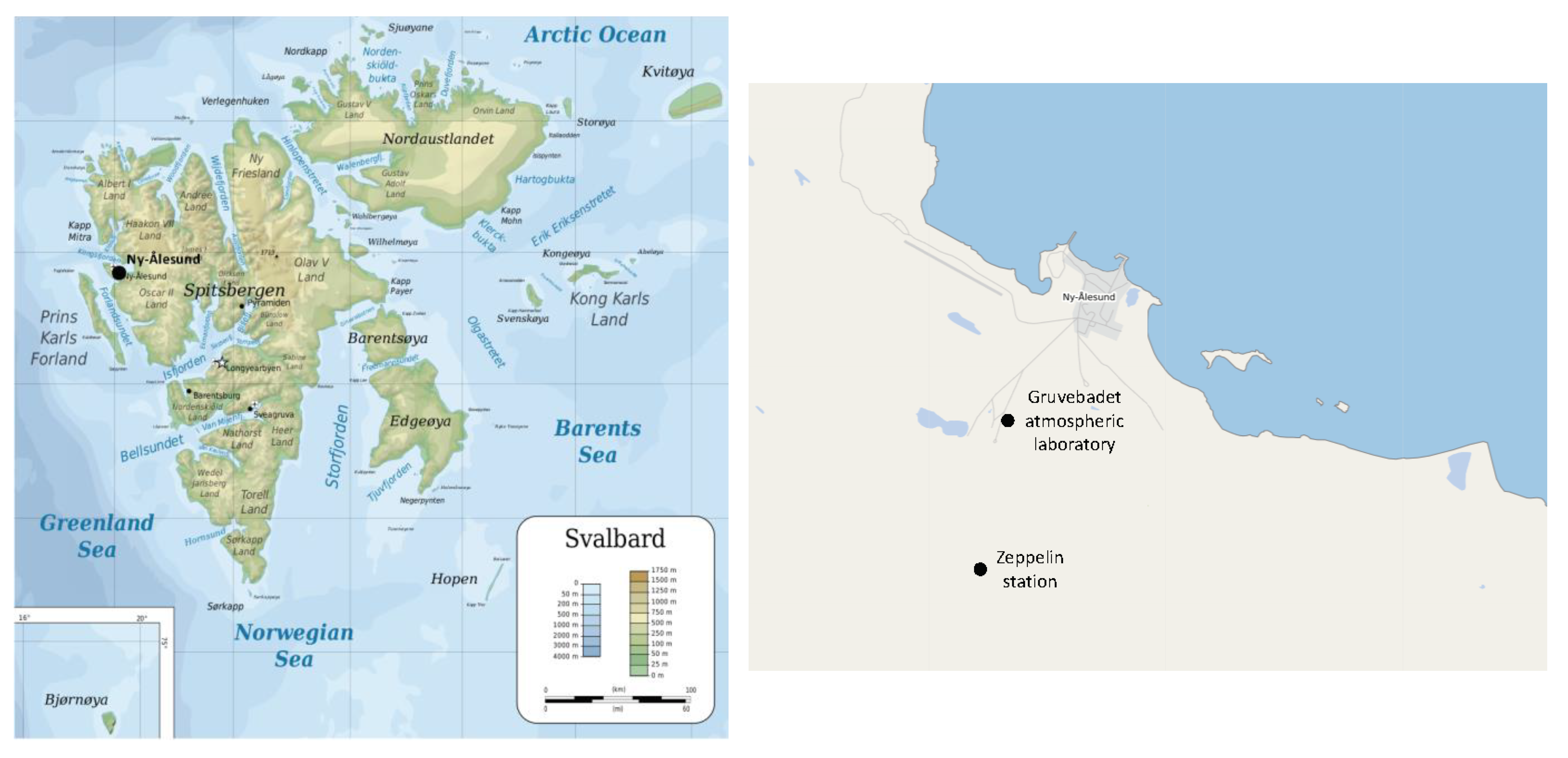
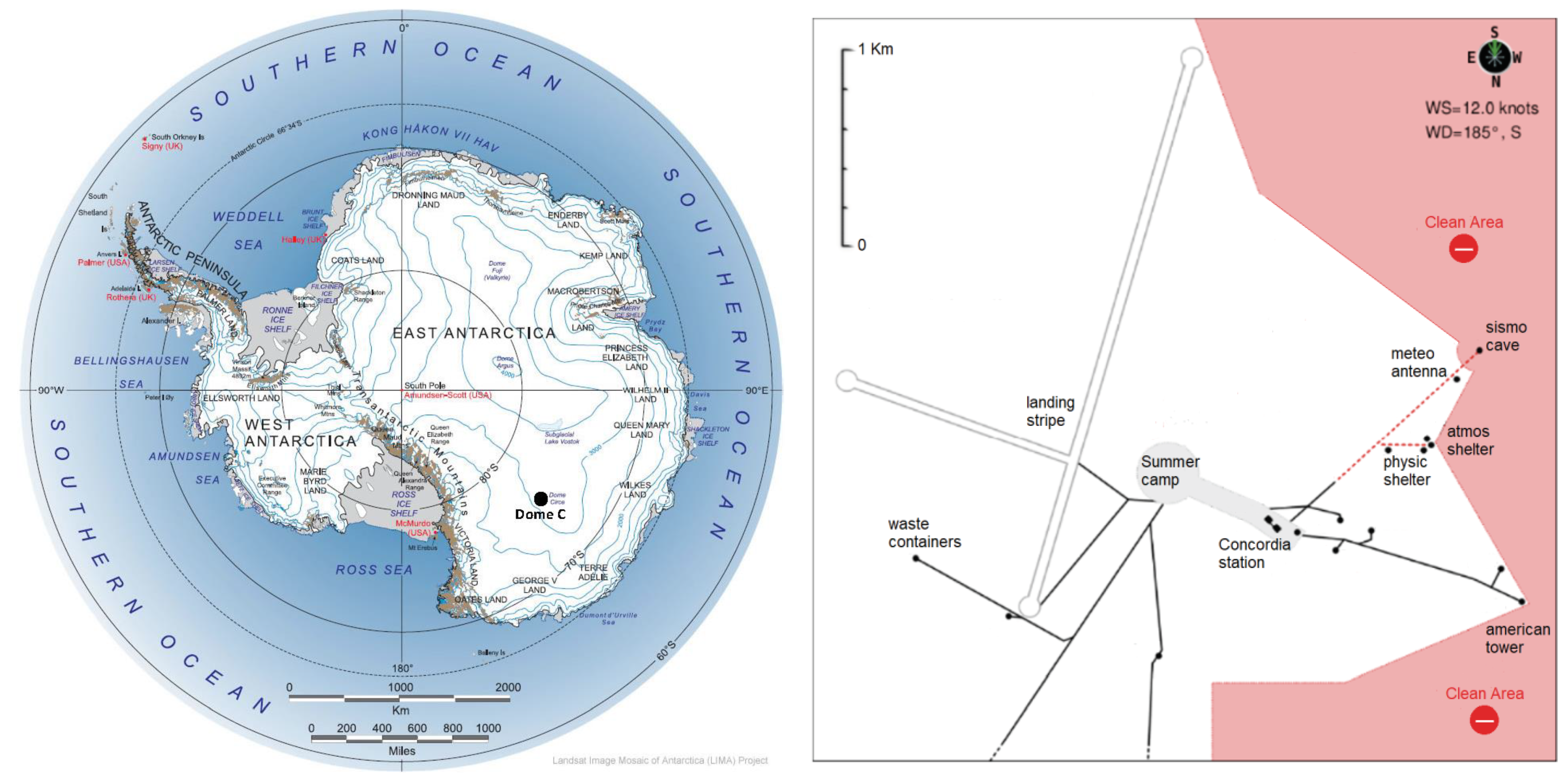
2.1. Sampling Sites
2.2. Sampling Instrumentation and Substrata
3. The Thermal-Optical Analysis
4. Improvements in the Sampling Strategies
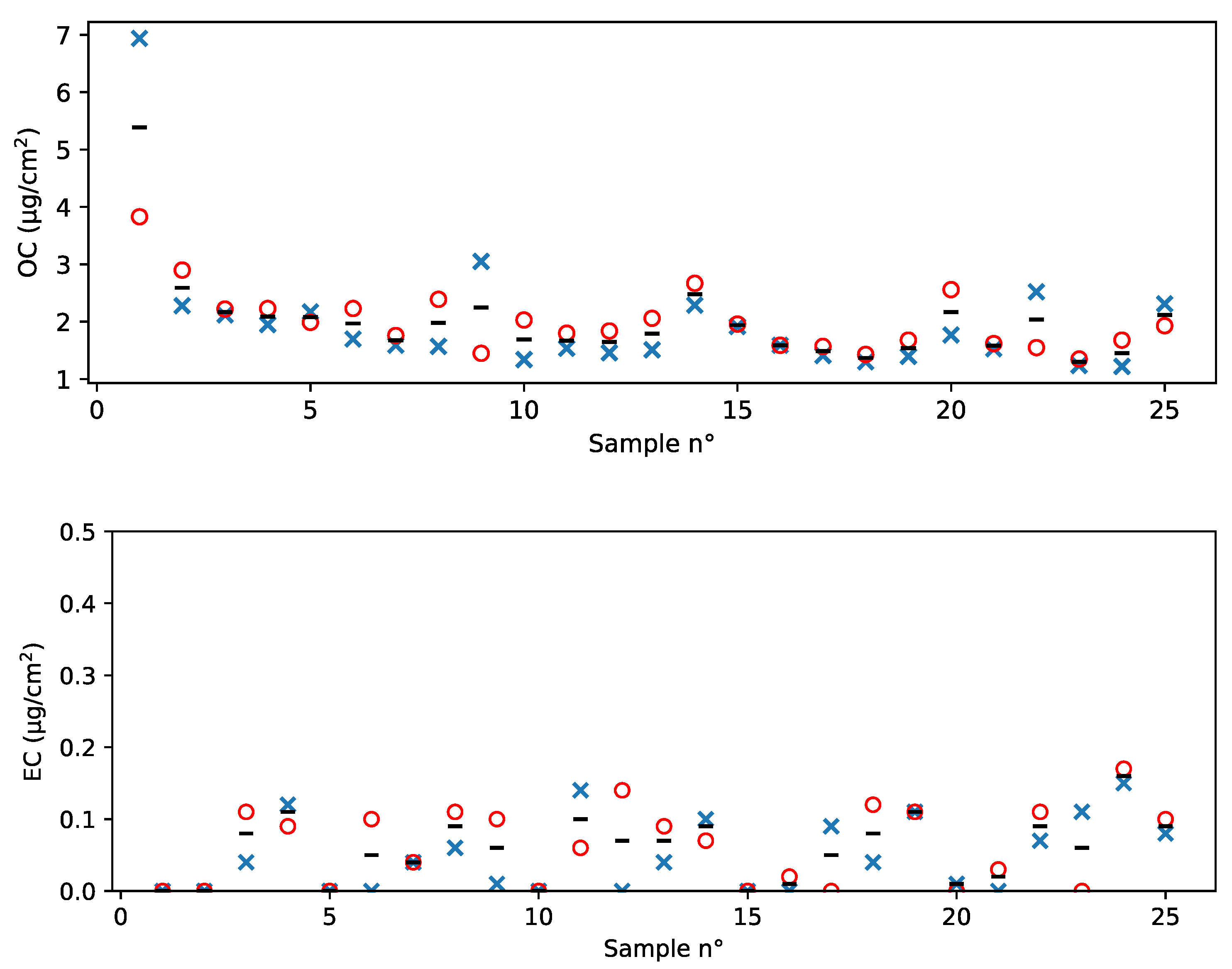
4.1. Analytical Performance and Blank Levels
4.2. Innovative Sampling Strategies
5. Results from Polar Samples
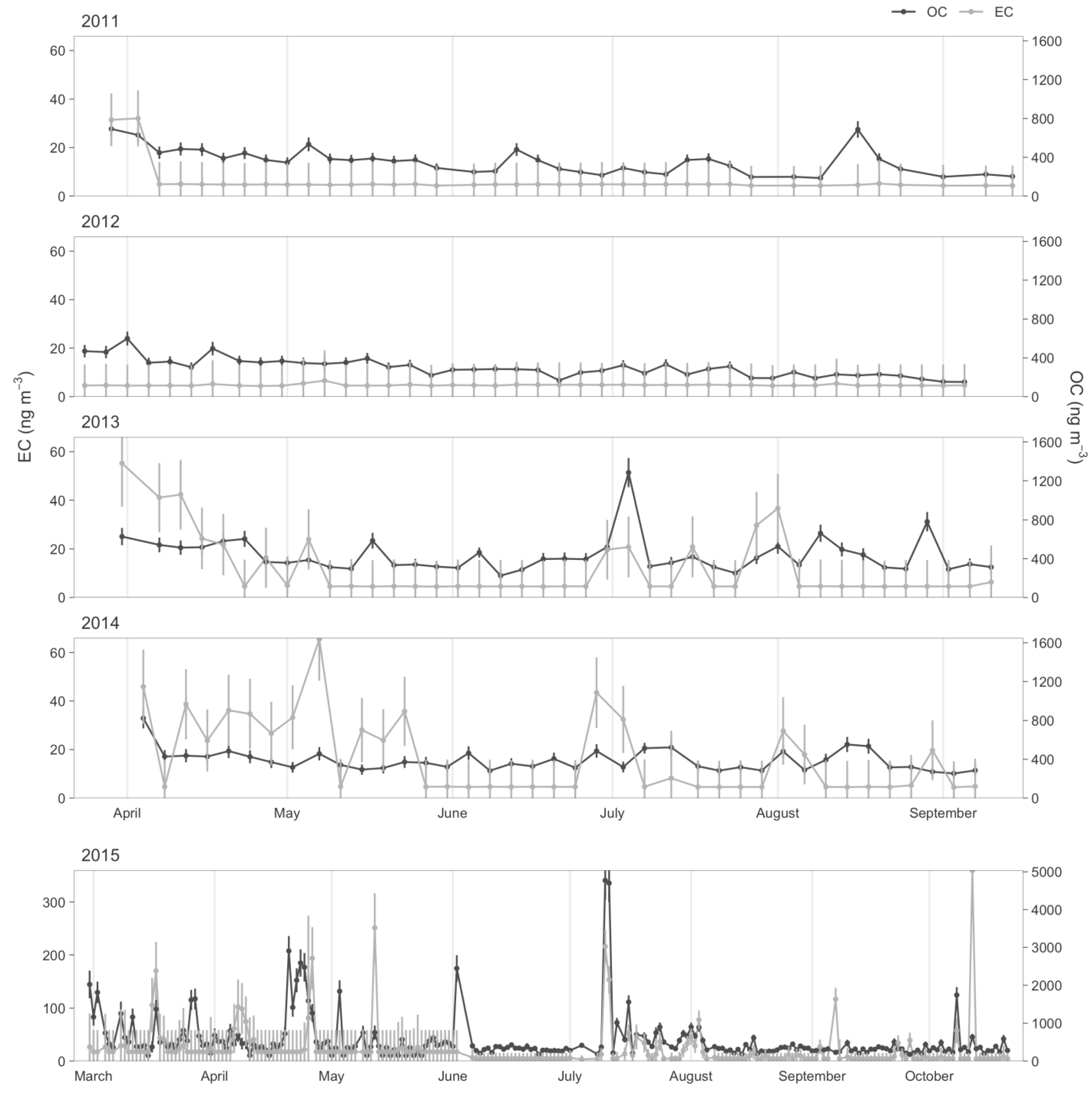
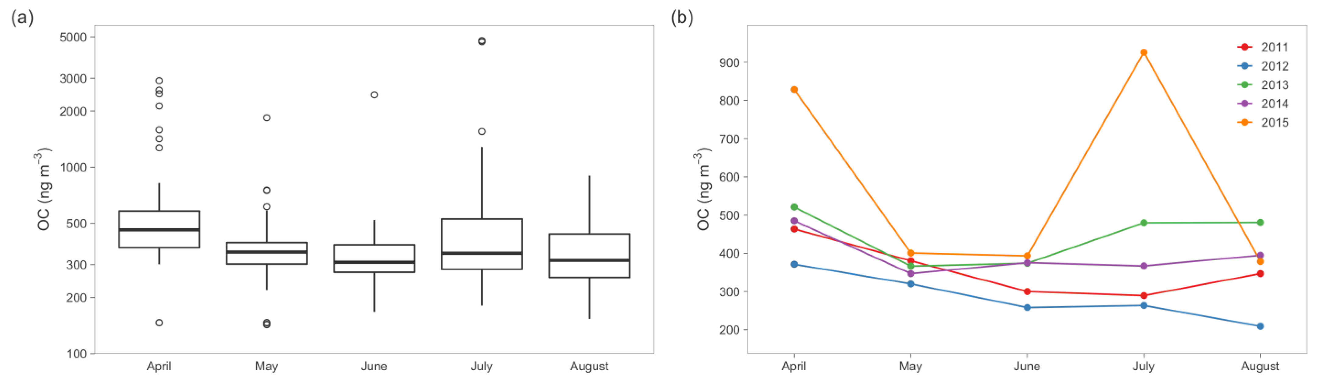
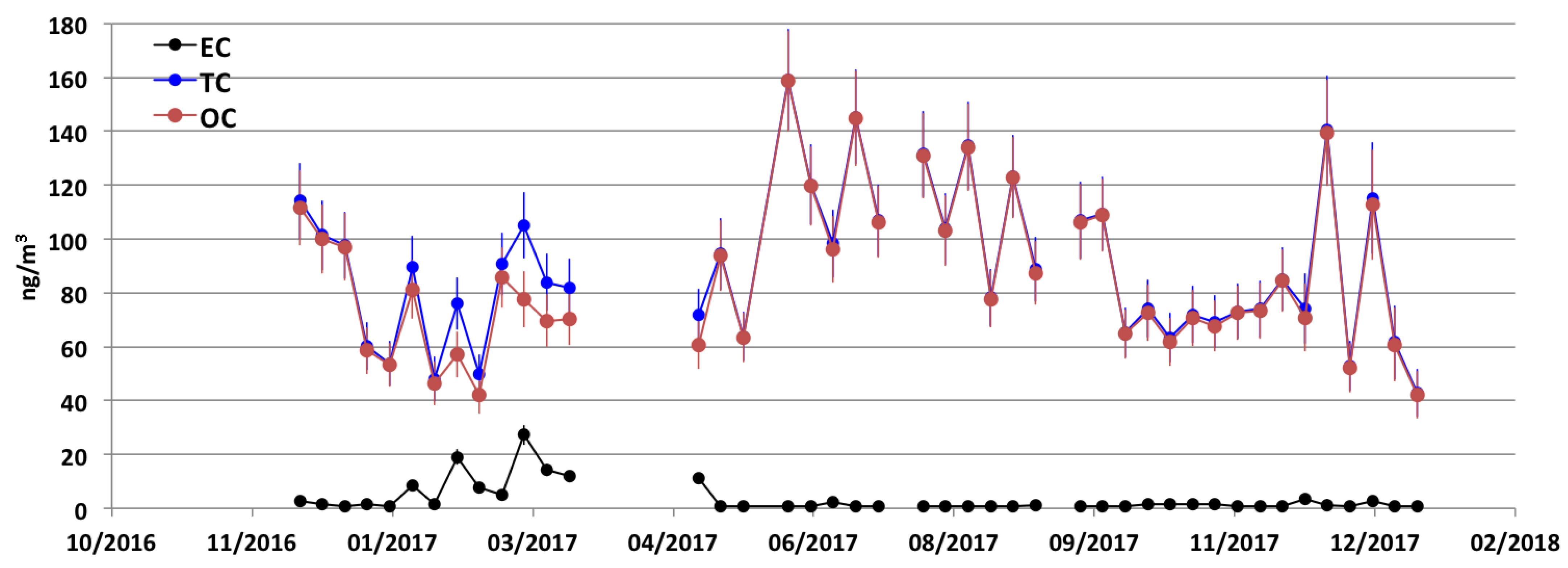
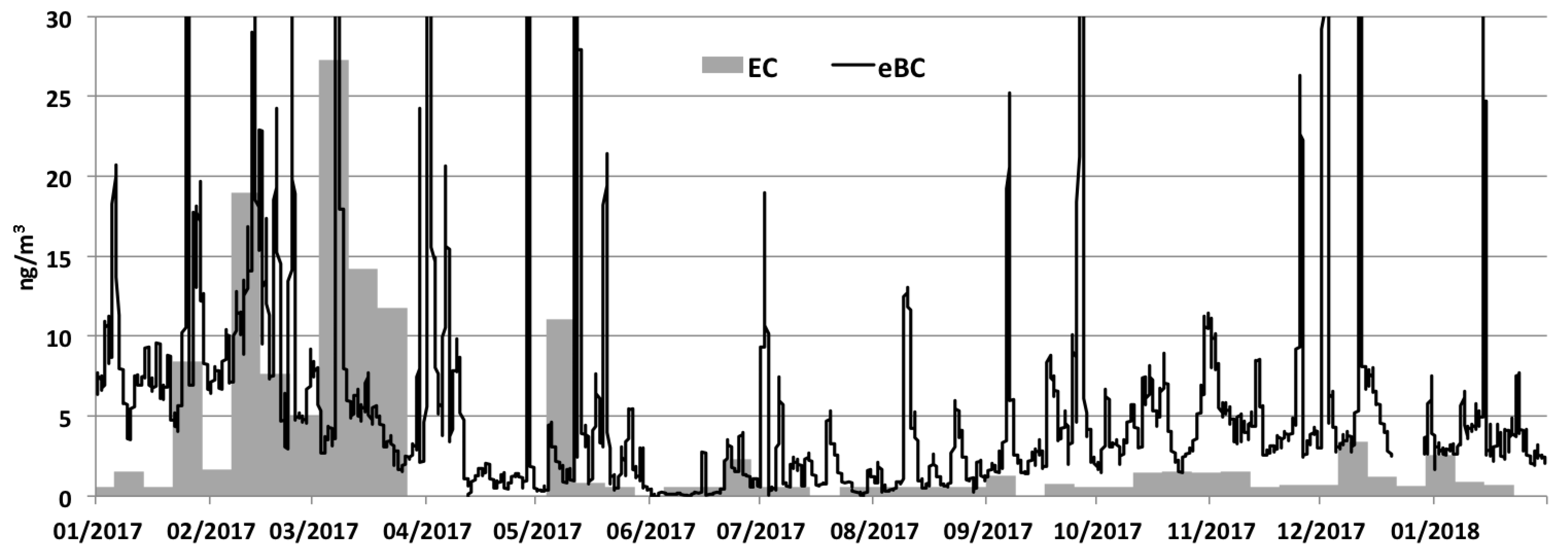
5.1. Arctic
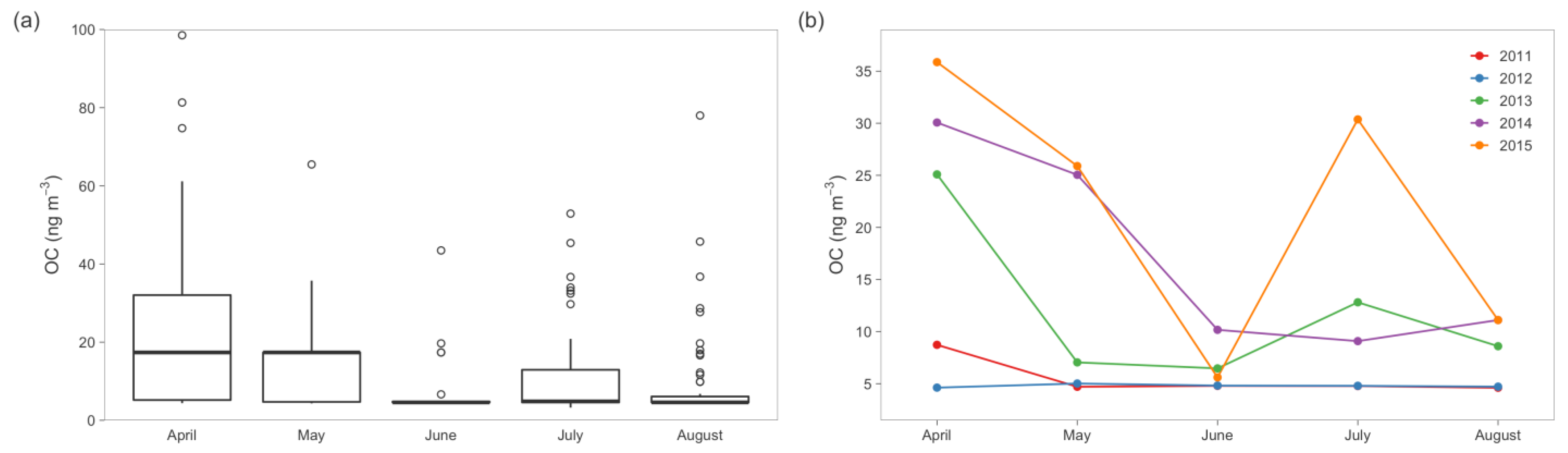
5.2. Antarctica
6. Conclusions
Author Contributions
Funding
Data Availability Statement
Acknowledgments
Conflicts of Interest
References
- Charlson, R.J.; Schwartz, S.E.; Hales, J.M.; Cess, R.D.; Coakley, J.A., Jr.; Hansen, J.E.; Hofmann, D.J. Climate forcing by anthropogenic aerosols. Science 1992, 255, 423–430. [Google Scholar] [CrossRef] [PubMed]
- Schulz, M.; Textor, C.; Kinne, S.; Balkanski, Y.; Bauer, S.; Berntsen, T.; Berglen, T.; Boucher, O.; Dentener, F.; Guibert, S.; et al. Radiative forcing by aerosols as derived from the AeroCom present-day and pre-industrial simulations. Atmos. Chem. Phys. Discuss. 2006, 6, 5225–5246. [Google Scholar] [CrossRef]
- Schwartz, S.E.; Arnold, F.; Blanchet, J.P.; Gurkee, P.A.; Hofmann, D.J.; Hoppel, W.A.; King, M.D.; Lacis, A.A.; Nakajima, T.; Ogren, J.A.; et al. Group report: Connections between aerosol properties and forcing of climate. In Aerosol Forcing of Climate; Charlson, R.J., Heintzenberg, J., Eds.; John Wiley: New York, NY, USA, 1995; pp. 251–280. [Google Scholar]
- Hansen, J.; Sato, M.; Lacis, A.; Ruedy, R. The missing climate forcing. Philos. Trans. R. Soc. B Biol. Sci. 1997, 352, 231–240. [Google Scholar] [CrossRef]
- Boucher, O.; Randall, D.; Artaxo, P.; Bretherton, C.; Feingold, G.; Forster, P.; Kerminen, V.M.; Kondo, Y.; Liao, H.; Lohmann, U.; et al. Clouds and Aerosols. In Climate Change the Physical Science Basis. Contribution of Working Group I to the Fifth Assessment Report of the Intergovernmental Panel on Climate Change; Stocker, T.F., Qin, D., Plattner, G.K., Tignor, M., Allen, S.K., Boschung, J., Nauels, A., Xia, Y., Bex, V., Midgley, P.M., Eds.; Cambridge University Press: Cambridge, UK; New York, NY, USA, 2013. [Google Scholar]
- Fermo, P.; Piazzalunga, A.; Vecchi, R.; Valli, G.; Ceriani, M. A TGA/FT-IR study for measuring OC and EC in aerosol samples. Atmos. Chem. Phys. Discuss. 2006, 6, 255–266. [Google Scholar] [CrossRef]
- Giannoni, M.; Calzolai, G.; Chiari, M.; Cincinelli, A.; Lucarelli, F.; Martellini, T.; Nava, S. A comparison between thermal-optical transmittance elemental carbon measured by different protocols in PM2.5 samples. Sci. Total. Environ. 2016, 571, 195–205. [Google Scholar] [CrossRef] [PubMed]
- Barrett, T.E.; Robinson, E.M.; Usenko, S.; Sheesley, R.J. Source Contributions to Wintertime Elemental and Organic Carbon in the Western Arctic Based on Radiocarbon and Tracer Apportionment. Environ. Sci. Technol. 2015, 49, 11631–11639. [Google Scholar] [CrossRef]
- Highwood, E.J.; Kinnersley, R.P. When smoke gets in our eyes: The multiple impacts of atmospheric black carbon on climate, air quality and health. Environ. Int. 2006, 32, 560–566. [Google Scholar] [CrossRef]
- Adar, S.D.; Kaufman, J.D. Cardiovascular disease and air pollutants: Evaluating and improving epidemio-logical data implicating traffic exposure. Inhal. Toxicol. 2007, 19, 135–149. [Google Scholar] [CrossRef]
- Bérubé, K.; Balharry, D.; Sexton, K.; Koshy, L.; Jones, T. Combustion-derived nanoparticles: Mechanisms of pul-monary toxicity. Clin. Exp. Pharmacol. P. 2007, 34, 1044–1050. [Google Scholar] [CrossRef]
- Winton, M. Amplified Arctic climate change: What does surface albedo feedback have to do with it? Geophys. Res. Lett. 2006, 33, 3. [Google Scholar] [CrossRef]
- Ramanathan, V.; Ramana, M.V.; Roberts, G.; Kim, D.; Corrigan, C.; Chung, C.; Winker, D.M. Warming trends in Asia amplified by brown cloud solar absorption. Nat. Cell Biol. 2007, 448, 575–578. [Google Scholar] [CrossRef]
- Rosen, H.; Novakov, T.; Bodhaine, B. Soot in the Arctic. Atmos. Environ. 1981, 15, 1371–1374. [Google Scholar] [CrossRef]
- Clarke, A.D.; Noone, K.J. Soot in the Arctic snowpack: A cause for perturbations in radiative transfer. Atmos. Environ. 1985, 19, 2045–2053. [Google Scholar] [CrossRef]
- Hansen, J.; Nazarenko, L. Soot climate forcing via snow and ice albedos. Proc. Natl. Acad. Sci. USA 2003, 101, 423–428. [Google Scholar] [CrossRef]
- Flanner, M.G.; Zender, C.S.; Randerson, J.T.; Rasch, P.J. Present-day climate forcing and response from black carbon in snow. J. Geophys. Res. Space Phys. 2007, 112, 1202. [Google Scholar] [CrossRef]
- Jacobson, M.Z. Strong radiative heating due to the mixing state of black carbon in atmospheric aerosols. Nat. Cell Biol. 2001, 409, 695–697. [Google Scholar] [CrossRef] [PubMed]
- Ramanathan, V.; Carmichael, G. Global and regional climate changes due to black carbon. Nat. Geosci. 2008, 1, 221–227. [Google Scholar] [CrossRef]
- Huebert, B.J.; Charlson, R.J. Uncertainties in data on organic aerosols. Tellus B Chem. Phys. Meteorol. 2000, 52, 1249–1255. [Google Scholar] [CrossRef]
- Jacobson, M.C.; Hansson, H.C.; Noone, K.J.; Charlson, R.J. Organic atmospheric aerosols: Review and state of the science. Rev. Geophys. 2000, 38, 267–294. [Google Scholar] [CrossRef]
- Turpin, B.J.; Huntzicker, J.J.; Hering, S.V. Investigation of organic aerosol sampling artifacts in the los angeles basin. Atmos. Environ. 1994, 28, 3061–3071. [Google Scholar] [CrossRef]
- Karanasiou, A.; Minguillón, M.C.; Viana, M.; Alastuey, A.; Putaud, J.P.; Maenhaut, W.; Panteliadis, P.; Močnik, G.; Favez, O.; Kuhlbusch, T.A.J. Thermal-optical analysis for the measurement of elemental carbon (EC) and organic carbon (OC) in ambient air a literature review. Atmos. Meas. Tech. Discuss. 2015, 8, 9649–9712. [Google Scholar] [CrossRef]
- Panteliadis, P.; Hafkenscheid, T.L.; Cary, B.; Diapouli, E.; Fischer, A.J.; Favez, O.; Inc, S.L.; Viana, M.M.; Hitzenberger, R.; Vecchi, R.; et al. ECOC comparison exercise with identical thermal protocols after temperature offset correction–instrument diagnostics by in-depth evaluation of operational parameters. Atmos. Meas. Tech. 2015, 8, 779–792. [Google Scholar] [CrossRef]
- Eleftheriadis, K.; Vratolis, S.; Nyeki, S. Aerosol black carbon in the European Arctic: Measurements at Zeppelin station, Ny-Ålesund, Svalbard from 1998. Geophys. Res. Lett. 2009, 36. [Google Scholar] [CrossRef]
- Sharma, S.; Lavoué, D.; Cachier, H.; Barrie, L.A.; Gong, S.L. Long-term trends of the black carbon concentrations in the Canadian Arctic. J. Geophys. Res. Space Phys. 2004, 109. [Google Scholar] [CrossRef]
- Sharma, S.; Andrews, E.; Barrie, L.A.; Ogren, J.A.; Lavoué, D. Variations and sources of the equivalent black carbon in the high Arctic revealed by long-term observations at Alert and Barrow: 1989. J. Geophys. Res. Space Phys. 2006, 111. [Google Scholar] [CrossRef]
- Sharma, S.; Barrie, L.; Magnusson, E.; Brattström, G.; Leaitch, W.; Steffen, A.; Landsberger, S. A Factor and Trends Analysis of Multidecadal Lower Tropospheric Observations of Arctic Aerosol Composition, Black Carbon, Ozone, and Mercury at Alert, Canada. J. Geophys. Res. Atmos. 2019, 124, 14133–14161. [Google Scholar] [CrossRef]
- Bodhaine, B.A. Aerosol absorption measurements at Barrow, Mauna Loa and the south pole. J. Geophys. Res. Space Phys. 1995, 100, 8967–8975. [Google Scholar] [CrossRef]
- Hansen, A.D.A.; Bodhaine, B.A.; Dutton, E.G.; Schnell, R.C. Aerosol black carbon measurements at the South Pole: Initial results, 1986. Geophys. Res. Lett. 1988, 15, 1193–1196. [Google Scholar] [CrossRef]
- Hansen, A.D.A.; Conway, T.J.; Strele, L.P.; Bodhaine, B.A.; Thoning, K.W.; Tans, P.; Novakov, T. Correlations among combustion effluent species at Barrow, Alaska: Aerosol black carbon, carbon dioxide, and methane. J. Atmos. Chem. 1989, 9, 283–299. [Google Scholar] [CrossRef]
- Hansen, A.D.; Lowenthal, D.H.; Chow, J.C.; Watson, J.G. Black carbon aerosol at McMurdo Station, Antarctica. J. Air Waste Manag. Assoc. 2001, 51, 593–600. [Google Scholar] [CrossRef]
- Von Schneidemesser, E.; Schauer, J.J.; Hagler, G.S.; Bergin, M.H. Concentrations and sources of carbonaceous aerosol in the atmosphere of Summit, Greenland. Atmos. Environ. 2009, 43, 4155–4162. [Google Scholar] [CrossRef]
- Virkkula, A.; Teinilä, K.; Hillamo, R.; Kerminen, V.-M.; Saarikoski, S.; Aurela, M.; Viidanoja, J.; Paatero, J.; Koponen, I.K.; Kulmala, M. Chemical composition of boundary layer aerosol over the Atlantic Ocean and at an Antarctic site. Atmos. Chem. Phys. Discuss. 2006, 6, 3407–3421. [Google Scholar] [CrossRef]
- Wolff, E.W.; Cachier, H. Concentrations and seasonal cycle of black carbon in aerosol at a coastal Antarctic station. J. Geophys. Res. Space Phys. 1998, 103, 11033–11041. [Google Scholar] [CrossRef]
- Weller, R.; Minikin, A.; Petzold, A.; Wagenbach, D.; Langlo, K.G. Characterization of long-term and seasonal variations of black carbon (BC) concentrations at Neumayer, Antarctica. Atmos. Chem. Phys. Discuss. 2013, 13, 1579–1590. [Google Scholar] [CrossRef]
- Winiger, P.; Andersson, A.; Yttri, K.E.; Tunved, P.; Gustafsson, Ö. Isotope-Based Source Apportionment of EC Aerosol Particles during Winter High-Pollution Events at the Zeppelin Observatory, Svalbard. Environ. Sci. Technol. 2015, 49, 11959–11966. [Google Scholar] [CrossRef]
- Winiger, P.; Andersson, A.; Eckhardt, S.; Stohl, A.; Gustafsson, Ö. The sources of atmospheric black carbon at a European gateway to the Arctic. Nat. Commun. 2016, 7, 2776. [Google Scholar] [CrossRef]
- Ferrero, L.; Cappelletti, D.; Busetto, M.; Mazzola, M.; Lupi, A.; Lanconelli, C.; Becagli, S.; Traversi, R.; Caiazzo, L.; Giardi, F.; et al. Vertical profiles of aerosol and black carbon in the Arctic: A seasonal phenomenology along 2 years (2011–2012) of field campaigns. Atmos. Chem. Phys. Discuss. 2016, 16, 12601–12629. [Google Scholar] [CrossRef]
- Spolaor, A.; Barbaro, E.; Mazzola, M.; Viola, A.P.; Lisok, J.; Obleitner, F.; Markowicz, K.M.; Cappelletti, D. Determination of black carbon and nanoparticles along glaciers in the Spitsbergen (Svalbard) region exploiting a mobile platform. Atmos. Environ. 2017, 170, 184–196. [Google Scholar] [CrossRef]
- Zhan, J.; Gao, Y.; Li, W.; Chen, L.; Lin, H.; Lin, Q. Effects of ship emissions on summertime aerosols at Ny–Alesund in the Arctic. Atmos. Pollut. Res. 2014, 5, 500–510. [Google Scholar] [CrossRef]
- Mazzera, D.M.; Lowenthal, D.H.; Chow, J.C.; Watson, J.G.; Grubĭsíc, V. PM10 measurements at McMurdo Station, Antarctica. Atmos. Environ. 2001, 35, 1891–1902. [Google Scholar] [CrossRef]
- Mazzera, D.M.; Lowenthal, D.H.; Chow, J.C.; Watson, J.G. Sources of PM10 and sulfate aerosol at McMurdo station, Antarctica. Chemosphere 2001, 45, 347–356. [Google Scholar] [CrossRef]
- Giardi, F.; Becagli, S.; Traversi, R.; Frosini, D.; Severi, M.; Caiazzo, L.; Ancillotti, C.; Cappelletti, D.; Moroni, B.; Grotti, M.; et al. Size distribution and ion composition of aerosol collected at Ny-Ålesund in the spring–summer field campaign. Rend. Lince 2016, 27, 47–58. [Google Scholar] [CrossRef]
- Udisti, R.; Becagli, S.; Frosini, D.; Ghedini, C.; Rugi, F.; Severi, M.; Traversi, R.; Zanini, R.; Calzolai, G.; Chiari, M.; et al. Activity and pre-liminary results from the 2011 and 2012 field seasons at Ny-Ålesund. In Research Activity in Ny Ålesund 2011-CNR Editions DTA/14-ISSN 2239–5172; Elsevier: Amsterdam, The Netherlands, 2016; pp. 53–68. [Google Scholar]
- Udisti, R.; Bazzano, A.; Becagli, S.; Bolzacchini, E.; Caiazzo, L.; Cappelletti, D.; Ferrero, L.; Frosini, D.; Giardi, F.; Grotti, M.; et al. Sulfate source apportionment in the Ny-Ålesund (Svalbard Islands) Arctic aerosol. Rend. Lince 2016, 27, 85–94. [Google Scholar] [CrossRef]
- Maturilli, M.; Herber, A.; Langlo, K.G. Climatology and time series of surface meteorology in Ny-Ålesund, Svalbard. Earth Syst. Sci. Data 2013, 5, 155–163. [Google Scholar] [CrossRef]
- Traversi, R.; Becagli, S.; Castellano, E.; Cerri, O.; Morganti, A.; Severi, M.; Udisti, R. Study of Dome C site (East Antartica) variability by comparing chemical stratigraphies. Microchem. J. 2009, 92, 7–14. [Google Scholar] [CrossRef]
- Turpin, B.J.; Cary, R.A.; Huntzicker, J.J. An in Situ, Time-Resolved Analyzer for Aerosol Organic and Elemental Carbon. Aerosol Sci. Technol. 1990, 12, 161–171. [Google Scholar] [CrossRef]
- Aswini, A.; Hegde, P.; Nair, P.R.; Aryasree, S. Seasonal changes in carbonaceous aerosols over a tropical coastal location in response to meteorological processes. Sci. Total. Environ. 2019, 656, 1261–1279. [Google Scholar] [CrossRef]
- Lack, D.A.; Moosmüller, H.; Mcmeeking, G.R.; Chakrabarty, R.K.; Baumgardner, D. Characterizing elemental, equivalent black, and refractory black carbon aerosol particles: A review of techniques, their limitations and uncertainties. Anal. Bioanal. Chem. 2014, 406, 99–122. [Google Scholar] [CrossRef] [PubMed]
- Chow, J.C.; Watson, J.G.; Crow, D.; Lowenthal, D.H.; Merrifield, T. Comparison of IMPROVE and NIOSH Carbon Measurements. Aerosol Sci. Technol. 2001, 34, 23–34. [Google Scholar] [CrossRef]
- Cheng, Y.; Duan, F.K.; He, K.B.; Zheng, M.; Du, Z.Y.; Ma, Y.L.; Tan, J.H. Intercomparison of Thermal–Optical Methods for the Determination of Organic and Elemental Carbon: Influences of Aerosol Composition and Implications. Environ. Sci. Technol. 2011, 45, 10117–10123. [Google Scholar] [CrossRef] [PubMed]
- Schmid, H.; Laskus, L.; Abraham, H.J.; Baltensperger, U.; Lavanchy, V.; Bizjak, M.; Burba, P.; Cachier, H.; Crow, D.; Chow, J.; et al. Results of the “carbon conference” international aerosol carbon round robin test stage I. Atmos. Environ. 2001, 35, 2111–2121. [Google Scholar] [CrossRef]
- Schauer, J.J.; Mader, B.T.; Deminter, J.T.; Heidemann, G.; Bae, M.S.; Seinfeld, J.H.; Flagan, R.C.; Cary, R.A.; Smith, D.; Huebert, B.J.; et al. ACE-Asia Intercomparison of a Thermal-Optical Method for the Determination of Particle-Phase Organic and Elemental Carbon. Environ. Sci. Technol. 2003, 37, 993–1001. [Google Scholar] [CrossRef] [PubMed]
- Ramachandran, S.; Khlystov, A.Y.; Robinson, A.L. Effect of Peak Inert-Mode Temperature on Elemental Carbon Measured Using Thermal-Optical Analysis. Aerosol Sci. Technol. 2006, 40, 763–780. [Google Scholar] [CrossRef]
- Sciare, J.; Oikonomou, K.; Favez, O.; Liakakou, E.; Markaki, Z.; Cachier, H.; Mihalopoulos, N. Long-term measurements of carbonaceous aerosols in the Eastern Mediterranean: Evidence of long-range transport of biomass burning. Atmos. Chem. Phys. Discuss. 2008, 8, 5551–5563. [Google Scholar] [CrossRef]
- Piazzalunga, A.; A Belis, C.; Bernardoni, V.; Cazzuli, O.; Fermo, P.; Valli, G.; Vecchi, R. Estimates of wood burning contribution to PM by the macro-tracer method using tailored emission factors. Atmos. Environ. 2011, 45, 6642–6649. [Google Scholar] [CrossRef]
- Birch, M.E.; Cary, R.A. Elemental Carbon-Based Method for Monitoring Occupational Exposures to Particulate Diesel Exhaust. Aerosol Sci. Technol. 1996, 25, 221–241. [Google Scholar] [CrossRef]
- Chow, J.C.; Watson, J.G.; Pritchett, L.C.; Pierson, W.R.; Frazier, C.A.; Purcell, R.G. The dri thermal/optical reflectance carbon analysis system: Description, evaluation and applications in U.S. Air quality studies. Atmos. Environ. Part A. Gen. Top. 1993, 27, 1185–1201. [Google Scholar] [CrossRef]
- Cavalli, F.; Putaud, J.P. Toward a standardized thermal-optical protocol for measuring atmospheric organic and elemental carbon: The EUSAAR protocol. Atmos. Meas. Tech. 2010, 3, 79–89. [Google Scholar] [CrossRef]
- Chow, J.C.; Watson, J.G.; Chen, L.W.A.; Chang, M.O.; Robinson, N.F.; Trimble, D.; Kohl, S. The IMPROVE_A Temperature Protocol for Thermal/Optical Carbon Analysis: Maintaining Consistency with a Long-Term Database. J. Air Waste Manag. Assoc. 2007, 57, 1014–1023. [Google Scholar] [CrossRef]
- Amato, F.; Alastuey, A.; Karanasiou, A.; Lucarelli, F.; Nava, S.; Calzolai, G.; Severi, M.; Becagli, S.; Gianelle, V.L.; Colombi, C.; et al. AIRUSE-LIFE+: A harmonized PM speciation and source apportionment in five southern European cities. Atmos. Chem. Phys. Discuss. 2016, 16, 3289–3309. [Google Scholar] [CrossRef]
- AMAP. The Impact of Black Carbon on Arctic Climate; Quinn, P.K., Stohl, A., Arneth, A., Berntsen, T., Burkhart, J.F., Christensen, J., Flanner, M., Kupiainen, K., Lihavainen, H., Shepherd, M., et al., Eds.; Arctic Monitoring and Assessment Programme (AMAP): Oslo, Norway, 2011; p. 72. [Google Scholar]
- AMAP Assessment. Black Carbon and Ozone as Arctic Climate Forcers; Arctic Monitoring and Assessment Programme (AMAP): Oslo, Norway, 2015; Volume 7, p. 116. [Google Scholar]
- Nielsen, I.E.; Skov, H.; Massling, A.; Eriksson, A.C.; Osto, D.M.; Junninen, H.; Sarnela, N.; Lange, R.; Collier, S.; Zhang, Q.; et al. Biogenic and anthropogenic sources of aerosols at the High Arctic site Villum Research Station. Atmos. Chem. Phys. Discuss. 2019, 19, 10239–10256. [Google Scholar] [CrossRef]
- Joranger, E.; Ottar, B. Air pollution studies in the Norwegian Arctic. Geophys. Res. Lett. 1984, 11, 365–368. [Google Scholar] [CrossRef]
- Tunved, P.; Ström, J.; Krejci, R. Arctic aerosol life cycle: Linking aerosol size distributions observed between 2000 and 2010 with air mass transport and precipitation at Zeppelin station, Ny-Ålesund, Svalbard. Atmos. Chem. Phys. Discuss. 2013, 13, 3643–3660. [Google Scholar] [CrossRef]
- Lampert, A.; Ström, J.; Ritter, C.; Neuber, R.; Yoon, Y.J.; Chae, N.Y.; Shiobara, M. Inclined lidar observations of boundary layer aerosol particles above the Kongsfjord, Svalbard. Acta Geophys. 2012, 60, 1287–1307. [Google Scholar] [CrossRef][Green Version]
- Moroni, B.; Cappelletti, D.; Crocchianti, S.; Becagli, S.; Caiazzo, L.; Traversi, R.; Udisti, R.; Mazzola, M.; Markowicz, K.; Ritter, C.; et al. Morphochemical characteristics and mixing state of long range transported wildfire particles at Ny-Ålesund (Svalbard Islands). Atmos. Environ. 2017, 156, 135–145. [Google Scholar] [CrossRef]
- Paxian, A.; Eyring, V.; Beer, W.; Sausen, R.; Wright, C. Present-Day and Future Global Bottum-Up Ship Emission Inventories Including Polar Routes. Environ. Sci. Technol. 2010, 44, 1333–1339. [Google Scholar] [CrossRef] [PubMed]
- Corbett, J.J.; Lack, D.A.; Winebrake, J.J.; Harder, S.; Silberman, J.A.; Gold, M. Arctic shipping emissions inventories and future scenarios. Atmos. Chem. Phys. Discuss. 2010, 10, 9689–9704. [Google Scholar] [CrossRef]
- Khon, V.C.; Mokhov, I.I.; Latif, M.; Semenov, V.A.; Park, W. Perspectives of Northern Sea Route and Northwest Passage in the twenty-first century. Clim. Chang. 2009, 100, 757–768. [Google Scholar] [CrossRef]
- Boé, J.; Hall, A.; Qu, X. September sea-ice cover in the Arctic Ocean projected to vanish. Nat. Geosci. 2009, 2, 341–343. [Google Scholar] [CrossRef]
- Peters, G.P.; Nilssen, T.B.; Lindholt, L.; Eide, M.S.; Glomsrød, S.; Eide, L.I.; Fuglestvedt, J.S.; Bergh, T. Future emissions from shipping and petroleum activities in the Arctic. Atmos. Chem. Phys. Discuss. 2011, 11, 5305–5320. [Google Scholar] [CrossRef]
- Eckhardt, S.; Hermansen, O.; Grythe, H.; Fiebig, M.; Stebel, K.; Cassiani, M.; Baecklund, A.; Stohl, A. The influence of cruise ship emissions on air pollution in Svalbard–A harbinger of a more polluted Arctic? Atmos. Chem. Phys. Discuss. 2013, 13, 8401–8409. [Google Scholar] [CrossRef]
- Vestreng, V.V.; Kallenborn, R.K.; Okstad, E.O. Norwegian Arctic Climate: Climate Influencing Emissions, Scenarios and Mitigation Options at Svalbard; Climate and Pollution Agency: Oslo, Norway.
- Weinbruch, S.; Wiesemann, D.; Ebert, M.; Schütze, K.; Kallenborn, R.; Ström, J. Chemical composition and sources of aerosol particles at Zeppelin Mountain (Ny Ålesund, Svalbard): An electron microscopy study. Atmos. Environ. 2012, 49, 142–150. [Google Scholar] [CrossRef]
- Lowenthal, D.H.; Zielinska, B.; Chow, J.C.; Watson, J.G.; Gautam, M.; Ferguson, D.H.; Neuroth, G.R.; Stevens, K.D. Characterization of heavy-duty diesel vehicle emissions. Atmos. Environ. 1994, 28, 731–743. [Google Scholar] [CrossRef]
- Na, K.; Sawant, A.A.; Song, C.; Cocker, D.R. Primary and secondary carbonaceous species in the atmosphere of Western Riverside County, California. Atmos. Environ. 2004, 38, 1345–1355. [Google Scholar] [CrossRef]
- Krecl, P.; Ström, J.; Johansson, C. Carbon content of atmospheric aerosols in a residential area during the wood combustion season in Sweden. Atmos. Environ. 2007, 41, 6974–6985. [Google Scholar] [CrossRef]
- Bond, T.C.; Anderson, T.L.; Campbell, D. Calibration and Intercomparison of Filter-Based Measurements of Visible Light Absorption by Aerosols. Aerosol Sci. Technol. 1999, 30, 582–600. [Google Scholar] [CrossRef]
- Ogren, J.A. Comment on “Calibration and Intercomparison of Filter-Based Measurements of Visible Light Absorption by Aerosols.”. Aerosol Sci. Technol. 2010, 44, 589–591. [Google Scholar] [CrossRef]


| MDL (µg/cm2) | MDL (ng/m3) | MDL (ng/m3) | MDL (ng/m3) | MDL (ng/m3) | |
|---|---|---|---|---|---|
| Filter diameter Sampled air volume | 47 mm 200 m3 | 47 mm 55 m3 | 25 mm 55 m3 | 25 mm 400 m3 | |
| OC | 1.35 | 80.3 | 292.1 | 77.4 | 10.6 |
| EC | 0.16 | 9.4 | 34.3 | 9.0 | 1.2 |
| Year | 2011 | 2012 | 2013 | 2014 | 2015 | 2011–2015 | |
|---|---|---|---|---|---|---|---|
| Sampling time (dd/mm) | 29/03–14/09 | 23/03–04/09 | 31/03–10/09 | 04/04–07/09 | 28/02–21/10 | ||
| Sampling resolution | 4 days | 4 days | 4 days | 4 days | daily | ||
| Diameter of the sampled filter (mm) | 47 | 47 | 47 | 47 | 47 (until 5/06) 25 (from 6/06) | ||
| OC | Mean ± σ (ng/m3) | 354 ± 132 | 296 ± 96 | 435 ± 185 | 386 ± 110 | 544 ± 606 553 ± 465 * | 470 ± 477 |
| Range (ng/m3) | 186–692 | 151–599 | 225–1285 | 253–823 | 143–4774 215–2676 * | Median: 352, IQR: 283–475 | |
| EC | Mean ± σ (ng/m3) | 6 ± 6 | 5 # | 12 ± 13 | 16 ± 16 | 22 ± 40 22 ± 23 * | 16 ± 32 |
| Range (ng/m3) | 5–32 | always < MDL | 4.5 #–55 | 4.5 #–65 | 3#–360 4 #–95 * | Median: 4.8, IQR: 4.6–17.4 | |
| TC | Mean ± σ (ng/m3) | 360 ± 136 | 301 ± 96 | 447 ± 190 | 403 ± 117 | 566 ± 624 575 ± 477 * | 486 ± 492 |
| Range (ng/m3) | 191–724 | 156–604 | 230–1305 | 258–868 | 161–4990 235–2771 * | Median: 360, IQR: 289–493 | |
Publisher’s Note: MDPI stays neutral with regard to jurisdictional claims in published maps and institutional affiliations. |
© 2021 by the authors. Licensee MDPI, Basel, Switzerland. This article is an open access article distributed under the terms and conditions of the Creative Commons Attribution (CC BY) license (http://creativecommons.org/licenses/by/4.0/).
Share and Cite
Caiazzo, L.; Calzolai, G.; Becagli, S.; Severi, M.; Amore, A.; Nardin, R.; Chiari, M.; Giardi, F.; Nava, S.; Lucarelli, F.; et al. Carbonaceous Aerosol in Polar Areas: First Results and Improvements of the Sampling Strategies. Atmosphere 2021, 12, 320. https://doi.org/10.3390/atmos12030320
Caiazzo L, Calzolai G, Becagli S, Severi M, Amore A, Nardin R, Chiari M, Giardi F, Nava S, Lucarelli F, et al. Carbonaceous Aerosol in Polar Areas: First Results and Improvements of the Sampling Strategies. Atmosphere. 2021; 12(3):320. https://doi.org/10.3390/atmos12030320
Chicago/Turabian StyleCaiazzo, Laura, Giulia Calzolai, Silvia Becagli, Mirko Severi, Alessandra Amore, Raffaello Nardin, Massimo Chiari, Fabio Giardi, Silvia Nava, Franco Lucarelli, and et al. 2021. "Carbonaceous Aerosol in Polar Areas: First Results and Improvements of the Sampling Strategies" Atmosphere 12, no. 3: 320. https://doi.org/10.3390/atmos12030320
APA StyleCaiazzo, L., Calzolai, G., Becagli, S., Severi, M., Amore, A., Nardin, R., Chiari, M., Giardi, F., Nava, S., Lucarelli, F., Pazzi, G., Cristofanelli, P., Virkkula, A., Gambaro, A., Barbaro, E., & Traversi, R. (2021). Carbonaceous Aerosol in Polar Areas: First Results and Improvements of the Sampling Strategies. Atmosphere, 12(3), 320. https://doi.org/10.3390/atmos12030320