Correction of Eddy Covariance Based Crop ET Considering the Heat Flux Source Area

Abstract

Eddy covariance (EC) systems are being used to measure sensible heat (H) and latent heat (LE) fluxes in order to determine crop water use or evapotranspiration (ET). The reliability of EC measurements depends on meeting certain meteorological assumptions; the most important of such are horizontal homogeneity, stationarity, and non-advective conditions. Over heterogeneous surfaces, the spatial context of the measurement must be known in order to properly interpret the magnitude of the heat flux measurement results. Over the past decades, there has been a proliferation of ‘heat flux source area’ (i.e., footprint) modeling studies, but only a few have explored the accuracy of the models over heterogeneous agricultural land. A composite ET estimate was created by using the estimated footprint weights for an EC system in the upwind corner of four fields and separate ET estimates from each of these fields. Three analytical footprint models were evaluated by comparing the composite ET to the measured ET. All three models performed consistently well, with an average mean bias error (MBE) of about −0.03 mm h⁻¹ (−4.4%) and root mean square error (RMSE) of 0.09 mm h⁻¹ (10.9%). The same three footprint models were then used to adjust the EC-measured ET to account for the fraction of the footprint that extended beyond the field of interest. The effectiveness of the footprint adjustment was determined by comparing the adjusted ET estimates with the lysimetric ET measurements from within the same field. This correction decreased the absolute hourly ET MBE by 8%, and the RMSE by 1%.

1. Introduction

Measuring and modeling ET is difficult due to the nature of water vapor transport into the atmosphere. Allen et al. [1] discussed the factors governing ET measurement accuracy for the following methods: 1. Soil water balance, 2. Lysimetry, 3. Energy Balance Bowen Ratio (EBBR), 4. Eddy Covariance (EC), 5. Scintillometry, 6. Sap flow, and 7. Remote sensing and satellite-based modeling. Soil water balance is an affordable and relatively accurate method that can be used for irrigation scheduling. However, for a novice or a person working outside their specialty, the errors in measurement can be 20–70% [1]. Methods 2–7 require expensive instrumentation and expert operators. Remote sensing and satellite-based modeling holds great potential for practical application, since the process covers large areas that can be instantaneously available via the internet. Sap flow methods directly measure the transpiration through a plant, but large errors are introduced when attempting to scale up measurements to a field or regional scale. Methods 2–5 are primarily used in research, and are being used to calibrate and validate remote sensing models. Properly managed lysimeters have the potential of measuring ET with high accuracy, according to Howell et al. [2]. However, these instruments are large, expensive, and only provide the user with a measurement that represents a rather small area. Methods 3 and 5 are micrometeorological approaches that are based on the conservation of energy. Since EC takes measurements above the transpiring canopy, the temperature and scalar concentrations sampled are actually a mixture of upwind point sources. The EC system has the advantage that it can be easily relocated, and that its derived sensible (H) and latent (LE) heat flux values are representative of the cropped field’s given heat flux source area.

1.1. Flux Footprint Modeling

The ‘heat flux source area’ (i.e., footprint) is the portion of the upwind surface of the EC instrumentation site containing the effective heat flux sources/sinks contributing to a flux or concentration observation at a certain measurement height [3,4]. If the EC system is located within the constant flux layer over an extended homogeneous surface, then the position of the sensor is not an issue. The extent of the footprint is significantly affected by the stability conditions of the atmosphere, and thus there is better energy balance closure under neutral to unstable conditions [5]. However, over a heterogeneous surface (e.g., a patchwork of agricultural land) the location and size of the flux footprint is needed to interpret the measured flux (i.e., to understand the source area of the heat fluxes). As a result, there has been a proliferation of footprint modeling research since 1990. There are four theoretical approaches: analytical models, Lagrangian-stochastic particle dispersion models, large-eddy simulations, and ensemble-averaged closure models [6,7]. The latter three approaches are mathematically complicated and thus resource intensive. Analytical models can be misleading if they are used in conditions that violate the underlying assumptions of each particular model [6,7]. Nevertheless, analytical models can easily be applied to processing code, and can thus be used to filter and correct flux measurements quickly in post-processing, or possibly in real time if they are programmed in the datalogger. The analytical footprint models of Hsieh et al. [8] and Kormann and Meixner [9] have been used as quality control filters for EC data collected over various land covers [10,11,12,13], and have been used to scale and validate remotely-sensed energy balance models [14,15,16]. The Kormann and Meixner model [9] is also employed by the frequently used open source EC data processing software EdiRe [17] and TK3 [18]. The intercomparison of footprint models was the primary method of validating footprint models in the past [8,19,20]. Foken and Leclerc [21] proposed three methods for the ‘in situ’ validation of models: (1) the use of artificial tracers, (2) the use of natural tracers, and (3) the effect of isolated heterogeneities. If a suitable artificial tracer is chosen, there is the advantage of there not being any other source or sink for the tracer. The disadvantages of artificial tracers are the difficulty of approximating natural field conditions and the expense of setting up these experiments. Natural tracer validation methods are both inexpensive and easier to use. Cooper [22] used water vapor as a natural tracer, and found good agreement between the point flux measurements of ET, lidar-derived water vapor fluxes, and a footprint model. By comparing the measurements from two adjoining surfaces and those of the two surfaces combined, Beyrich et al. [23] found that Lagrangian stochastic simulation [24] better represented the flux contribution from different fields than Schmid’s analytical model [25]. Marcolla and Cescatti [26] compared three analytical models by comparing measurements from an alpine meadow before and after cutting to those during an intermittent time when only a portion of the meadow was cut. As a result, they found that the Schuepp et al. [4] model generally overestimates the footprint, and that none of the footprint models considered perform well in very unstable atmospheric conditions.

1.2. Motivation and Objectives

Analytical footprint models have been extensively studied for different atmospheric conditions, and have been compared to other more sophisticated models (e.g., Lagrangian stochastic). Only a few studies have explored the accuracy of such models over irrigated cropland surrounded by rainfed crops and/or fallow land. Furthermore, there has not been a study that has explored the correction of flux measurements for a footprint that extends beyond the area of interest. Therefore, the objectives of this study are: (a) to compare the performance of the Schuepp et al. [4], Hsieh et al. [8] and Kormann and Meixner [9] analytical footprint models over irrigated cotton adjacent to dryland cotton; and (b) to develop and evaluate a method for improving the LE flux, measured by an EC system, by accounting for the footprint fraction that extends beyond the irrigated field boundaries.

2. Materials and Methods

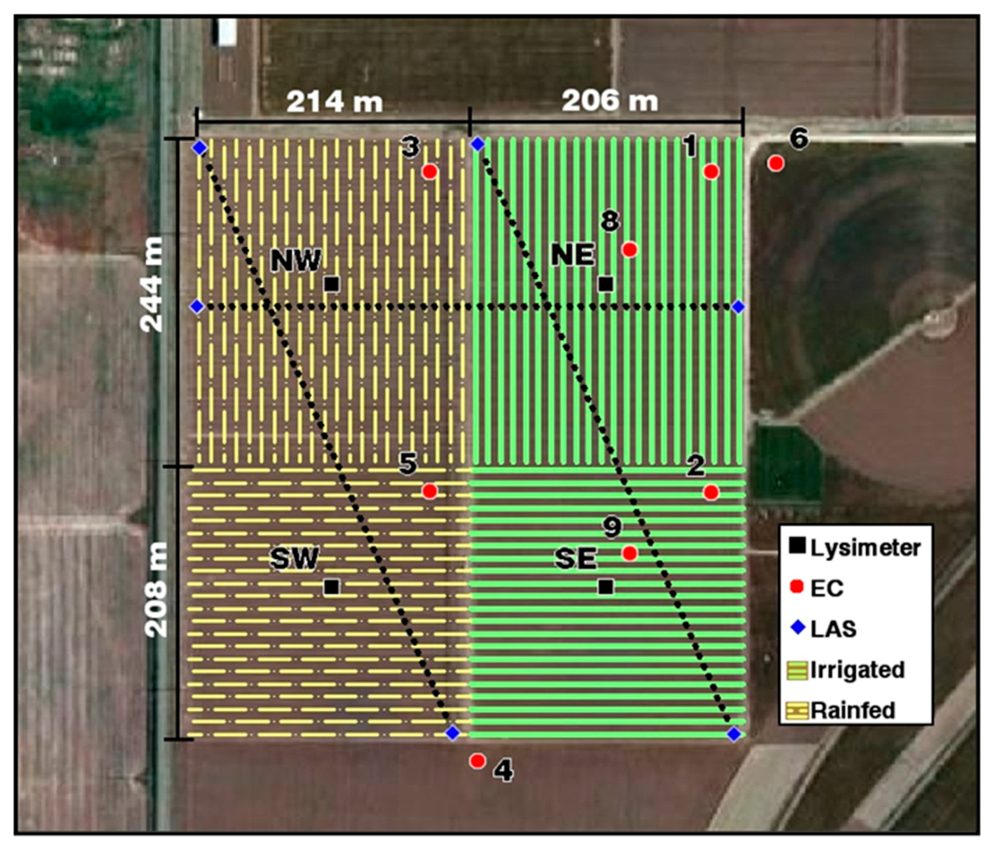
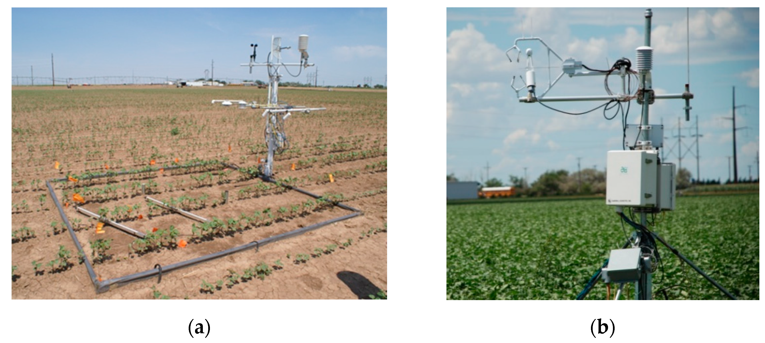
2.1. Site Description

For this study, data from the Bushland Evapotranspiration and Agricultural Remote Sensing Experiment 2008 (BEAREX08) was used [27]. The geographic coordinates of the USDA-ARS Conservation and Production Research Laboratory (CPRL), located at Bushland, TX, USA are 35°11′ N, 102°06′ W, and its elevation is 1170 m above mean sea level. The soils in and around Bushland are classified as slowly permeable Pullman clay loam. The major crops in the region are corn, sorghum, winter wheat, and cotton. The wind direction is predominantly from the south/southwest direction. The average precipitation that occurs during the cotton growing season (May–October) is 350 mm [28]. About 600 mm of irrigation, precipitation, and soil water are needed to grow cotton [29]; thus, irrigation needs to provide about 250 mm of timely water for a successful cotton harvest. The typical growing season grass reference ET is 6.0–8.2 mm/day⁻¹ [28]. In addition, the long-term annual microclimatological conditions indicate that the study area is subject to very dry air and strong winds. The growing season averages at Bushland for air temperature and horizontal wind speed are 20 °C and 3.9 m s⁻¹, respectively [28].

2.1.1. Large Monolith Weighing Lysimeters

Four precision weighing lysimeters [30], 3 × 3 × 2.3 m deep, were used to measure the cotton ET. Each lysimeter contained a monolithic Pullman clay loam soil core. The lysimeters were located at the center of four fields (210 m east–west by 225 m north–south), two (east) of which were irrigated by a linear move system, and two (west) of which were not irrigated. The change in the lysimeter mass was measured by a load cell (SM-50, Interface, Scottsdale, AZ, USA) and recorded by a datalogger (CR7-X, Campbell Scientific Inc., Logan, UT, USA) at a 0.17 Hz frequency. The high frequency load cell signal was averaged for 5 min and composited to 15-min means. The lysimeter was calibrated as explained in Howell et al. [2]. A simple soil water balance using the change in water storage from four neutron probes, irrigation, and precipitation data showed that the northeast (NE) lysimeter had a larger ET than the surrounding field [31]. According to that study, the ET measurements from the NE lysimeter were 18% larger than the surrounding field from Day of Year (DOY) 182 to 220, as determined by a soil water balance using the neutron probe soil water content readings, due to the greater leaf area index (LAI) on the lysimeter than the surrounding field. Therefore, the NE lysimeter ET measurements, from that period, were reduced by 18% in order to ensure that they were representative of the entire field, as indicated by Evett et al. [31]. Pictures of a lysimeter box and an EC system are shown in Figure 1.

2.1.2. Eddy Covariance Energy Balance System

Five EC systems (EC1, EC2, EC3, EC5, and EC8) out of the nine from the BEAREX08 experiment were used to monitor the exchange of heat fluxes at different parts of the CPRL site. The instrument positions are shown in Figure 2. The instrumentation details of all of the systems used are given in

Table 1. Instrumentation details for the eddy covariance systems and lysimeter.

Instrument	EC8	EC1, EC2, EC3, EC5	Lysimeters
3D Sonic Anemometer	CSAT3 1	CSAT3 1	—
Open Path Gas Analyzer	LI-7500 2	LI-7500 2	—
Fine Wire Thermocouple	FW05 1	FW05 1	—
Air Temp/Relative Humidity	HMP45C 3	HMP45C 3	HMP45C 3
Barometer	CS106 1	—	—
Net Radiometer	—	CNR1 5	REBS Q*7.1 4, KandZ CM14 5, KandZ CGR3 5
Soil Heat Flux Plates	(2) REBS HFT-3 4	(3) REBS HFT-1.1 4	(4) REBS HFT-1.1 4
Soil Temperature	(4) TCAV 1	(6) TMTSS-020G-6 6	(8) TMTSS-020G-6 6
Soil Water Content	(2) CS616 1	(3) CS616 1	—
Precipitation Gauge	—	—	Qualimetrics 6011B 7
Datalogger	CR3000 1	CR5000 1	CR7X 1
CSAT Azimuth	225°	180°	—
Measurement Height	2.5 m	2.25 m	—
Sampling frequency	20 Hz 7	20 Hz 7	0.17 Hz

¹ Campbell Scientific Inc., Logan, UT, USA. ^2. LI-COR Biosciences, Lincoln, NE, USA. ^3. Vaisala Inc., Woburn, MA, USA. ^4. Radiation and Energy Balance Systems, Bellevue, WA, USA. ^5. Kipp and Zonen USA, Bohemia, NY, USA. ^6. Omega Engineering Inc., Stamford, CT, USA. ^7. All Weather Inc., Sacramento, CA, USA.

. The time series data consisted of the horizontal (u), lateral (v), and vertical (w) wind vectors (m s⁻¹); calculated sonic temperature (T_s, °C); water vapor concentration (H₂O, g m⁻³); carbon dioxide concentration (CO₂, mg m⁻³); and atmospheric pressure (P, kPa), all measured at a frequency of 20 Hz. The Campbell Scientific 3-dimensional (3D) sonic anemometer (CSAT3) sensor was oriented toward the predominant wind direction, with an azimuth angle of 225° from true north for EC8, and 180° for systems EC1, EC2, EC3, and EC5. Installed within and between the crop rows, about 4 m east from each EC system, were instruments for measuring soil heat flux, soil temperature, and soil volumetric water content. The temperature and water content data were used to calculate the soil heat storage in the layer between the surface and the depth of the soil heat flux plate installation. The soil heat flux plates (SHFP) were installed at 0.08 m depth within and between the crop rows. The soil thermocouple pairs were installed at 0.02 and 0.07 m depths close to the SHFP locations. The soil water content reflectometers (CS616, Campbell Scientific Inc., Logan, UT, USA) were installed slanted at an approximate angle of 13 degrees across the 0.02–0.1 m depth, in order to measure the volumetric soil water content in this depth zone. The water content reflectometers were field cross-calibrated against the water contents reported by a conventional time domain reflectometry (TDR) (TR-100, Dynamax, Inc., Houston, TX, USA) system that used a soil-specific calibration that minimized soil temperature influences on the TDR water content readings [32]. Soil temperature was sensed and recorded during the cross-calibration, and a soil temperature correction was developed for the CS616 data (Personal communication, [33]).

2.2. Eddy Covariance Data Processing

The major components of the energy balance at the land surface are net radiation (R_n), soil heat flux (G), sensible heat flux (H), and latent heat flux (LE), all in units of W m⁻², and can be expressed as:

$$R_n-G=H+LE$$

(1)

where the left side in Equation (1) is defined as the available energy (R_n − G), and the right side is defined as the turbulent fluxes (H + LE), with the positive sign convention away from the surface for H and LE and negative for R_n and G. The EC method is based on the direct measurement of high-frequency vertical wind (w) and a scalar concentration (c), such as water vapor or air temperature, producing LE through Equation (2) and H through Equation (3), respectively, assuming that the mean vertical velocity is negligible:

$$LE={\rho }_a\lambda \overline{w^{\prime }{q}^{\prime }}$$

(2)

$$H=C_p{\rho }_a\overline{w^{\prime }{T}^{\prime }}$$

(3)

where q is the air-specific humidity (kg kg⁻¹); T is the air temperature (°C); ρ_a is the moist air density (kg m⁻³); C_p is the specific heat of dry air at constant pressure (J kg⁻¹ K⁻¹); λ is the latent heat of water vaporization (J kg⁻¹), which varies T; and the primes (apostrophes) denote the deviation or fluctuation from the mean (e.g., $x^{\prime }=x-\overline{x}$).

Time series, high-frequency EC data were post-processed with the EdiRe software package [17] following the guidelines described in Lee et al. [34] and Burba and Anderson [35], as summarized in

Table 2. Post-processing procedure using the software package EdiRe.

Procedure		EdiRe Commands
1	Extract raw time series data	Extract
2	Calculate wind direction	Wind direction
3	Remove spikes	Despike
4	Calculate and remove lag between instruments	Cross correlate, Remove lag
5	Rotate coordinates	Rotation coefficients, Rotation
6	Calculate means, standard deviations, skewness, and kurtosis	1 chn statistics
7	Calculate covariances and fluxes	Latent heat of evaporation, Sensible heat flux coefficient, 2 chn statistics
8	Calculate friction velocity and stability	User defined, Stability - Monin Obukhov
9	Calculate and apply frequency response corrections	Frequency response
10	Calculate and apply Schotanus H correction	Sonic T - heat flux correction
11	Calculate and apply WPL correction	Webb correction
12	Iterate steps 8–11 two times
13	Convert LE to ET (mm h−1)	User defined
14	Calculate roughness length	Roughness length (z0)
15	Calculate stationarity	Stationarity

. Before the covariances were calculated, spikes of six standard deviations from the population mean were removed from the time series. If four or more consecutive data points were detected with values larger than the standard deviation then they were not considered as a spike [36]. The time delay between the CSAT3 and LI-7500 was removed using a cross-correlation analysis [37]. Although the terrain for the site was practically flat, the CSAT3 cannot be perfectly leveled, such that the vertical component (w) is perpendicular to the mean streamline plane. For this reason, the coordinates were rotated using the double rotation method [38]. According to Lee et al. [34], this method is suitable for ideal sites with little slope and fair weather conditions. The effects of density fluctuations induced by heat fluxes on the measurement of the eddy fluxes of water vapor using the LI-7500 were corrected using the procedure outlined by Webb et al. [39]. The spectral loss in the high frequency band due to path-length averaging, sensor separation, and signal processing was corrected after Moore [40]. The data from the fine wire thermocouple was intermittent due to equipment failure, and thus the sonic temperature (T_s) was used in sensible heat flux calculation. Schotanus et al. [41] recommended correcting T_s for crosswind and humidity effects, which are commonly referred to as the heat flux correction. The CSAT3 implements the crosswind correction online, and therefore the heat flux only needed to be corrected for humidity fluctuations. The sonic temperature flux was converted to actual air temperature flux following the method of Schotanus et al. [41].

A dimensionless parameter that characterizes the processes in the surface layer is the atmospheric stability parameter (ζ), Equation (4), which is the ratio of the convective production to the mechanical production of turbulent kinetic energy [42]:

$$\zeta =-\frac{0.4z_{m}gH}{\left(T+273.15\right){\rho }_a{C}_p{u}_{*}^3}$$

(4)

where z_m is the horizontal wind speed observation height above the zero-plane displacement height (i.e., z_m = z − d); g is the gravitational acceleration (9.8 m s⁻²); u* is the friction velocity (m s⁻¹); and H, T, ρ_a, and C_p are as defined above. A positive ζ represents a stable stratification of the atmosphere, a negative ζ represents an unstable stratification, and |ζ | < 0.02 represents a neutral stratification.

The canopy heights (h_c, m) and leaf area index (LAI, m² m⁻²) for the NE and southeast (SE) fields were measured five times during the study, on the following days of the year (DOY): 171, 182, 200, 210, and 220. Field measurements were taken for the northwest (NW) and southwest (SW) fields three times, on DOYs 200, 210, and 220. The crop emergence for the east and west fields occurred on DOY 150 and 165, respectively. Curves were fitted to the h_c vs. DOY and LAI vs. DOY data in order to determine the h_c and LAI as functions of the DOY; these are shown in Appendix A. The analytical expression from Raupach [43,44,45] was used to estimate the zero-plane displacement height (d, m):

$$d=h_c-h_c\left[\frac{1-exp\left(-\sqrt{c_{d1}\Lambda }\right)}{\sqrt{c_{d1}\Lambda }}\right]$$

(5)

where c_d1 is an empirical constant estimated from laboratory and field data to be on the order of 7.5 [44], and Λ is the canopy area index, which for unstressed, growing canopies is equivalent to the LAI.

Quality control criteria were set for the wind direction, stationarity, and integral turbulence characteristics. The flow from behind the sensor can be distorted by the instrumentation. Therefore, any data with a wind direction beyond ±90° of the orientation of the sonic anemometer were excluded from further analysis. The estimates of fluxes via the eddy covariance method are based on simplified forms of the Navier–Stokes equations for certain atmospheric conditions [46]. These conditions are not always met, and therefore must be evaluated. The tests for stationarity and integral turbulence were performed following the methods outlined in Foken and Wichura [47], and Thomas and Foken [48].

2.3. Footprint Modeling Methodology

The analytical footprint models proposed by Schuepp et al. [4], Hsieh et al. [8], and Kormann and Meixner [9] were used to determine the footprint weight for each hourly flux per unit source area (i.e., 1 m × 1 m), hereafter referred to as S90, H2000, and KM01, respectively. This was achieved by first rotating into the mean wind direction the respective x and y coordinates of a 450 × 420 grid, with each point representing one square meter (i.e., the size of the entire four-field site) centered at the position of each EC system. The rotated coordinates were then used to calculate the relative footprint contribution of each point on the grid. The footprint contribution of each field was then found by creating a 450 by 420 matrix for each field, which consisted of 1 s and 0 s, with the 1 s representing the area of interest; multiplying each of those respective matrices by the matrix of footprint density weights; and then summing all of the elements of the final matrix. The MATLAB codes, following this procedure for each footprint model, are shown in Appendix B and Appendix C.

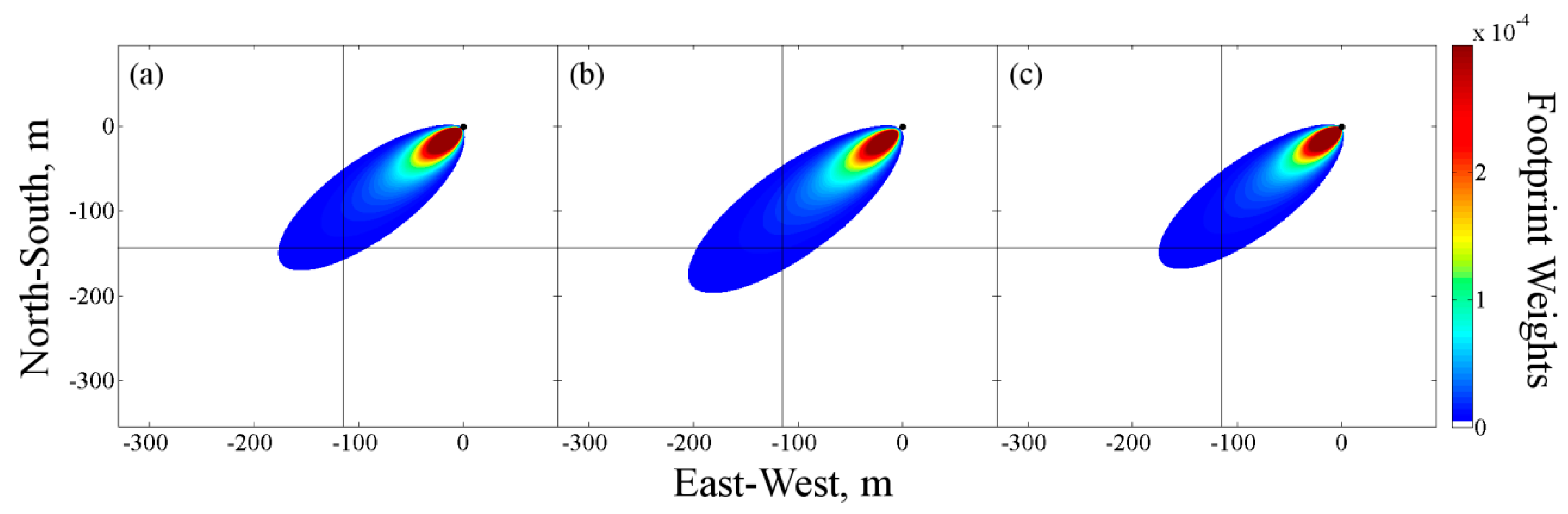
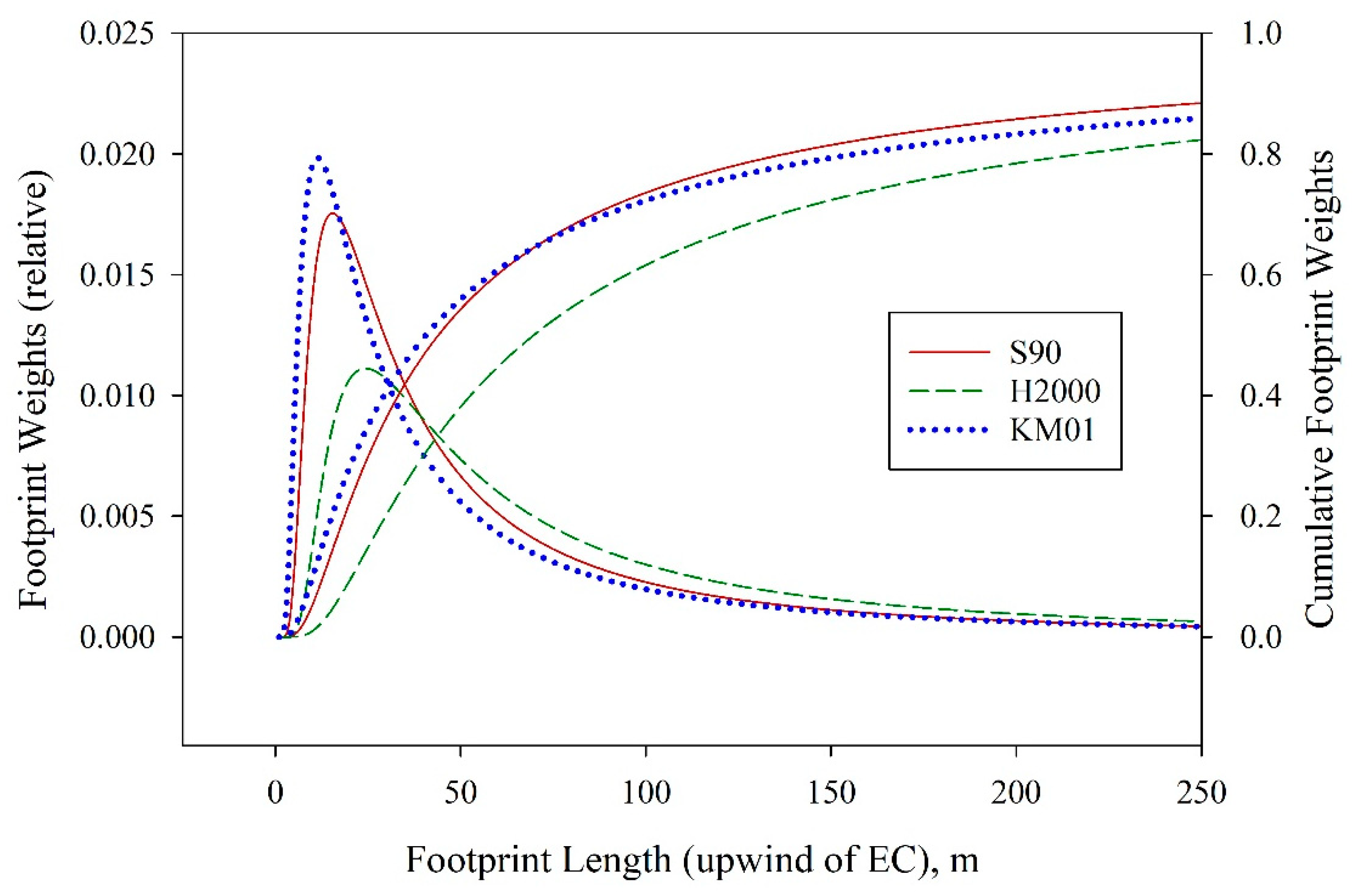
2.3.1. Schuepp Model

The S90 model views the transpiring vegetative surface as a continuum of upwind line sources, each occupying an infinitesimal strip of width δx. As proposed by Gash [49], the approximate analytical solution by Calder [50] was applied to the basic advection–diffusion equation, assuming neutral stability and uniform wind velocity. After differentiating with respect to z_m and then integrating with respect to the upwind distance (x), an equation for the vertical concentration gradient at z_m is reached:

$$\frac{\partial {\rho }_v\left(z_m\right)}{\partial z_m}=-\frac{Q_0}{k{u}_{*}{z}_m}exp\left(-\frac{U{z}_m}{k{u}_{*}x}\right)$$

(6)

where k is von Kármán’s constant (0.41), Q₀ is the area flux density, and U is the uniform wind velocity (m s⁻¹), which is defined as the average wind velocity between the surface and z_m (m), assuming a logarithmic profile for u(z):

$$U=\frac{u_{*}\left[ln\left(z_m/z_0\right)-1+z_0/z_m\right]}{k\left(1-z_0/z_m\right)}$$

(7)

where z₀ is the surface roughness length (m). The relative contribution to the vertical flux at height z_m, f(x,z_m), is then obtained by taking the derivative of Equation (6) and multiplying by ku*z_m:

$$f\left(x,z_m\right)=\frac{k{u}_{*}{z}_m\left(d\rho /dz\right)}{Q_0}=\frac{U{z}_m{\varphi }_M}{k{u}_{*}{x}^2}exp\left(-\frac{U{z}_m{\varphi }_M}{k{u}_{*}x}\right)$$

(8)

where ϕ_M is the momentum correction for stability, which is a function of Monin–Obukhov stability parameter ζ [51].

$${\varphi }_M=\{\begin{array}{c}{\left(1-16\zeta \right)}^{-1/4}\\ 1+5\zeta \end{array}\begin{array}{c}for \zeta <0\\ for \zeta >0\end{array}$$

(9)

2.3.2. Hsieh Model

The H2000 model is a hybrid approach which fits Calder’s analytical solution [50] to the results of the numerical Lagrangian model of Thomson [52]. In the analysis of their results, Hsieh et al. [8] scaled Gash’s [49] effective fetch with the Monin–Obukhov stability length (L, m), and accounted for the effects of stability by introducing the similarity parameters D and P, so that:

$$\frac{x}{\left|L\right|}=-\frac{D{\left(\raisebox{1ex}{$z_u$}\!\left/ \!\raisebox{-1ex}{$\left|L\right|$}\right.\right)}^P}{k^{2}ln\left(F\right)}$$

(10)

with

$$z_u=z_m\left[ln\left(z_m/z_0\right)-1+z_0/z_m\right]$$

(11)

where D and P are found by the regression of Equation (10) to the Lagrangian model results for unstable (D = 0.28, P = 0.59), near-neutral (D = 0.97, P = 1), and stable stratification (D = 2.44, P = 1.33). Rearranging Equation (10) and differentiating with respect to x results in the analytical footprint expression:

$$f\left(x,z_m\right)=\frac{D{z}_u{}^P{\left|L\right|}^{\left(1-P\right)}}{k^2{x}^2}exp\left(-\frac{D{z}_u{}^P{\left|L\right|}^{\left(1-P\right)}}{k^{2}x}\right)$$

(12)

2.3.3. Crosswind Function

Both S90 and H2000 are one-dimensional (1D) footprint models (i.e., they are expressed along the mean wind direction (x)). The KM01 model is a two-dimensional (2D) model that expresses the footprint in the mean wind direction and the crosswind direction (y). The S90 and H2000 models were expanded into 2D models, so that the results could be compared to KM01. The diffusion in the lateral direction is commonly assumed to have a Gaussian distribution centered on the mean wind direction:

$$D_y\left(x,y\right)=\frac{1}{\sqrt{2\pi }{\sigma }_y}exp\left(-\frac{y^2}{2{\sigma }_y{}^2}\right)$$

(13)

where D_y is the crosswind concentration distribution function, and σ_y is the standard deviation of the lateral spread of the source area, which can be related to the plume travel time, x/ū_p, and the standard deviation of lateral wind fluctuations, σ_v as σ_y ≈ σ_v∙x/ū_p [9,16,53,54]. The Gaussian distribution was combined with H2000 and S90 to expand them into 2D footprint models:

$$f\left(x,y,z_m\right)=f\left(x,z_m\right)D_y\left(x,y\right)$$

(14)

2.3.4. Kormann and Meixner Model

The KM01 model uses the solution of the resulting two-dimensional advection–diffusion equation for the power law profiles of the mean wind velocity and the eddy diffusivity. The mathematical framework is a stationary gradient diffusion formulation with height-independent crosswind dispersion. The profile parameters are determined by equating the power law to Monin–Obukhov similarity profiles. The complete mathematical description is given by Kormann and Meixner [9]. However, a condensed set of formulas similar to that presented by Neftel et al. [55] is presented here. First, the profiles of the horizontal wind speed and the vertical eddy diffusivity are described by power law relationships:

$$u\left(z\right)={\alpha }_u{z}^m$$

(15)

$$K\left(z\right)={\alpha }_{\kappa }{z}^n$$

(16)

The proportionality constants α_u and α_κ, and the exponents m and n are determined by comparing Equation (15) and (16) to the respective Monin–Obukhov similarity profiles at height z_m:

$$m=\frac{u_{*}{\varphi }_M}{ku}$$

(17)

$$n=\frac{z_m}{K}\frac{dK}{d{z}_m}=\{\begin{array}{c}\frac{1}{1+5\varsigma }\\ \frac{1-24\varsigma }{1-16\varsigma }\end{array}\begin{array}{c}for \varsigma <0\\ \\ for \varsigma >0\end{array}$$

(18)

$${\alpha }_u=\frac{u_{*}{\varphi }_M}{km{\left(z_m\right)}^m}$$

(19)

$${\alpha }_{\kappa }=\frac{k{u}_{*}{z}_M}{{\varphi }_H{\left(z_m\right)}^n}$$

(20)

where ϕ_H is the dimensionless gradient function of the heat profile defined by Dyer [51] as:

$${\varphi }_H=\{\begin{array}{c}{\left(1-16\varsigma \right)}^{-1/2}\\ 1+5\varsigma \end{array}\begin{array}{c}for \varsigma <0\\ for \varsigma >0\end{array}$$

(21)

Based on these quantities, the shape factor r and the constant μ of Equations (22) and (23) are defined as:

$$r=2+m-n$$

(22)

$$\mu =\frac{1+m}{r}$$

(23)

Finally, the parameters A–E, shown below, are related to the above quantities:

$$A=1+\mu$$

(24)

$$B=\frac{{\alpha }_u{\left(z_m\right)}^r}{r^2{\alpha }_{\kappa }}$$

(25)

$$C=\frac{B^{\mu }}{\Gamma \left(\mu \right)}$$

(26)

$$D=\frac{{\sigma }_v}{{\alpha }_u}\frac{\Gamma \left(1/r\right)}{\Gamma \left(\mu \right)}{\left(\frac{{\alpha }_u}{r^2{\alpha }_{\kappa }}\right)}^{m/r}$$

(27)

$$E=\frac{r-m}{r}$$

(28)

The 3D flux footprint can then be expressed as:

$$f\left(x,y,z_m\right)=\frac{1}{\sqrt{2\pi }D{x}^E}exp\left[-\frac{y^2}{2{\left(D{x}^E\right)}^2}\right]C{x}^{-A}exp\left(-\frac{B}{x}\right)$$

(29)

The first half of the equation is the Gaussian crosswind distribution, and the second half is the crosswind-integrated longitudinal distribution.

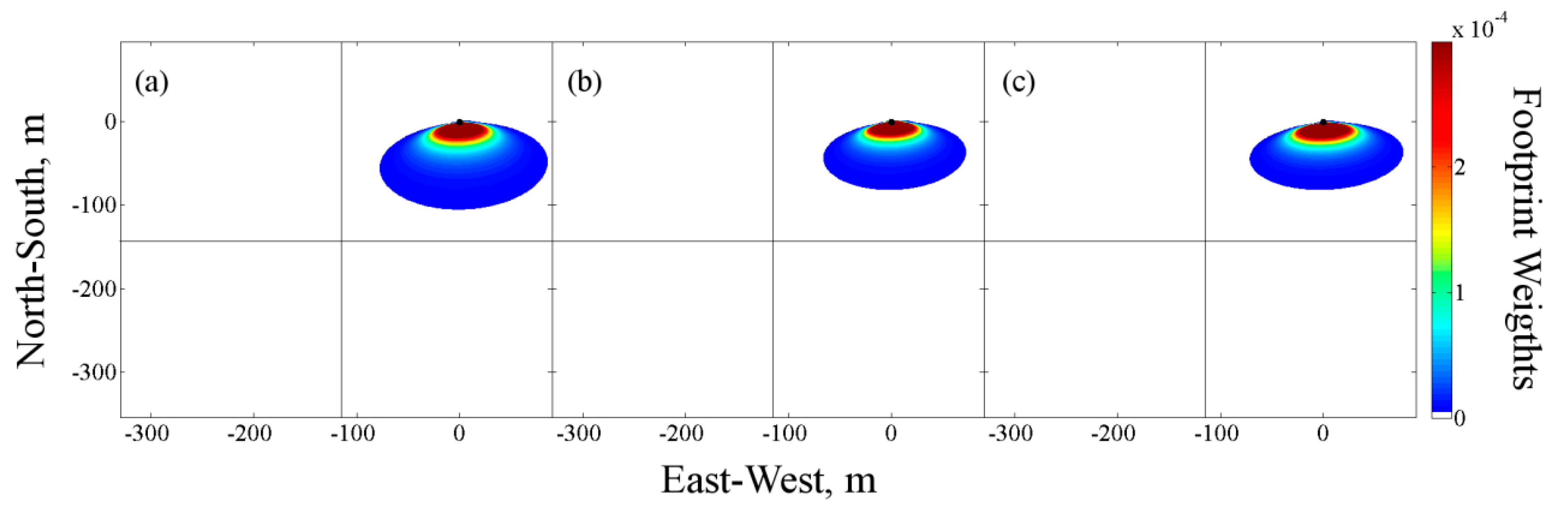
2.4. Footprint Validation Procedure

The premise of the validation of footprint models using water vapor as a natural tracer is that if the footprint model correctly estimates the footprint weight for each element of the heat flux source area, then those elemental footprint weights represent a fraction of the EC-derived ET. If, then, the ET for each element of the heat flux source area can be accurately measured by another method, the sum of the products of the footprint weights and their respective EC-based ET rates should equal that of the independently-measured ET value. Following that premise, the cumulative footprint within each of the fields was used to calculate a composite ET (ET_composite) which was then compared to the measured ET value at EC8:

$$E{T}_{composite}=F_{NE}\times E{T}_{EC1}+F_{NW}\times E{T}_{EC3}+F_{SW}\times E{T}_{EC5}+F_{SE}\times E{T}_{EC2}$$

(30)

where F is the cumulative footprint fraction for each field (the subscripts indicate the field), and ET_EC1, ET_EC3, ET_EC5, and ET_EC2 are the EC-based ET (mm h⁻¹) from EC1, EC3, EC5, and EC2, respectively.

The underlying assumption is that the surface conditions within each field are homogeneous. In order to ensure that the EC-based ET values from each field were representative of the field, an infield cumulative footprint fraction limit was set. The selection of the footprint fraction limit was based on the optimization of the exclusion of the EC data that had significant influence from areas outside of the field, while still retaining enough data for the analysis. A minimum 80% of the footprint for EC1, EC3, EC5, and EC2 must come from the NE, NW, SW, and SE fields, respectively.

2.5. ET Correction Using Footprint Fractions

When the footprint for a heat flux measurement extends beyond the field of interest, the flux (measured by the EC system) is then influenced by the surrounding area heat fluxes. During the summer of 2008, the east fields were irrigated, and as a result the ET from those fields was greater than that from the west fields. Therefore, any contribution to the flux from the west fields would be cause for an underestimation of the EC-based ET for the east fields. Using the same footprint limit as in the validation procedure, the ET at EC8 was corrected for the footprint fraction extending beyond the NE field using the model shown below:

$$\begin{array}{c}E{T}_{FC}=E{T}_{EC8}+F_{NW}dE{T}_{EC3}+F_{SW}dE{T}_{EC5}+F_{SE}dE{T}_{EC2}\\ +\left[1-\left(F_{NE}+F_{NW}+F_{SW}+F_{SE}\right)\right]E{T}_{EC8}\end{array}$$

(31)

where ET_FC is the corrected ET (at EC8 location), considering footprint weights, and dET_i is the difference in ET between the ith EC and EC8 systems:

$$dE{T}_i=E{T}_{EC8}-E{T}_i$$

(32)

The contribution from adjacent fields to the ET measured by EC8 is removed by the terms dET_EC3, dET_EC5, and dET_EC2 in Equation (32), while the latter part of the equation removes any contribution to the ET at EC8 that is not accounted for in the adjacent NW, SW, and SE fields, based on the assumption that there is little to no ET from the area extending beyond the four fields, and thus dET = ET_EC8-0. The effectiveness of the adjustment was determined by comparing ET_FC to the ET measurements from the NE lysimeter.

2.6. Statistical Analysis

The mean bias error (MBE), the root mean square error (RMSE), and the linear regression analysis based on the least squares method for the comparison of a fitted equation slope and intercept were used for the comparison of ET values [56,57]:

$$MBE=\frac{1}{N}{\displaystyle \sum }_{i=1}^N\left(P_i-O_i\right)$$

(33)

where N is the number of pairs compared, P_i is the predicted or corrected value, and O_i is the observed value.

$$RMSE=\sqrt{\frac{1}{N}{\displaystyle \sum }_{i=1}^N{\left(P_i-O_i\right)}^2}$$

(34)

3. Results and Discussion

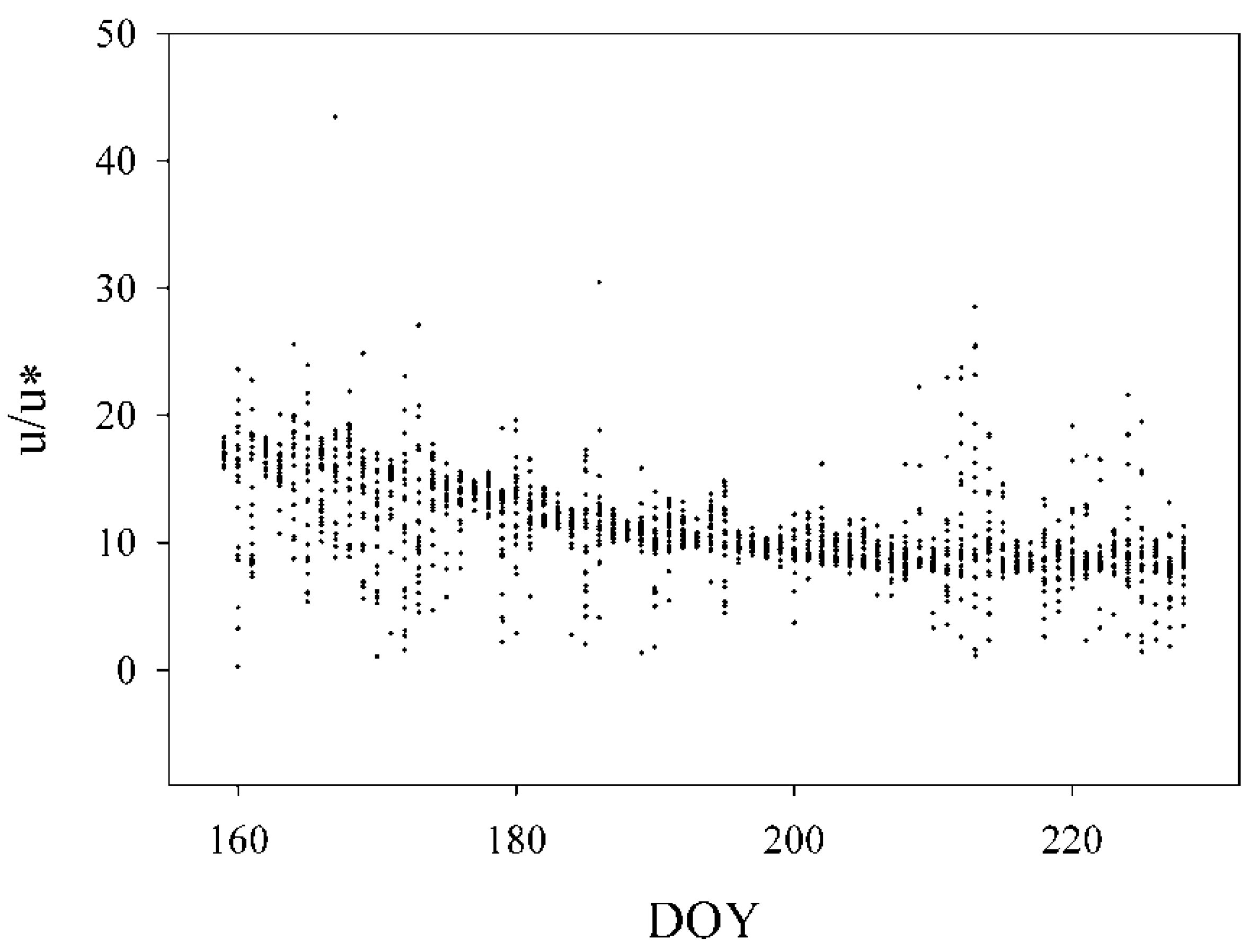
3.1. Surface Roughness

Because the crop height and LAI were derived from five spot measurements throughout the study period, it is necessary to evaluate the spatial homogeneity of each field. An underlying assumption for all three of the analytical footprint models presented here is that the surface is spatially homogenous for the extent (fetch) of the footprint. This condition is rarely met when measuring fluxes over agricultural lands due to the typical patchwork of fields, each with a different crop, surface roughness, and water availability. Although it is the objective of this study to ascertain the effectiveness of analytical footprint models over such terrain, each field within this study needs to be reasonably homogeneous in order to properly estimate the composite ET. There are many factors that contribute to the spatial variability of a field (e.g., soil type, irrigation and/or rainfall spatial uniformity, topography, soil fertility, agro-chemical spatial application uniformity, plant germination, etc.). However, a good indicator of the combined effect of these conditions is the vegetation biomass status. Using remote sensing data, the amount of vegetation cover can be determined via the normalized difference vegetation index (NDVI). The NDVI is calculated using visible (VIS) red (R) and near-infrared (NIR) light reflected by the vegetation, and it varies from −1 to 1 [58]. The pigment in plant leaves, chlorophyll, strongly absorbs visible light (in the bandwidth 0.4 to 0.7 µm of the electro-magnetic spectrum) for use in photosynthesis. The cell structure of the leaves, on the other hand, strongly reflects near-infrared light (from 0.7 to 1.1 µm). The more leaves a plant has, the more these wavelengths of light are affected, respectively. The USA National Aeronautics and Space Administration’s (NASA) Landsat 5 thematic mapper satellite operates on a 16-day acquisition schedule, in which an image will be captured of any given surface every 16 days. The satellite reflectance images of the site for the stated study period were obtained using the online Earth Explorer tool [59], and NDVI calculations were performed. Three of the nine images covering the crop growth period could not be used due to excessive cloud cover. The remaining six images are shown in Figure 3 (spatial pixel size of 30 m × 30 m). The vegetative cover was uniform over all of the fields, with a mean NDVI of 0.24 and a standard deviation (SD) of 0–0.01 (0.0–4.7%) during the period between DOYs 155 and 171 (Figure 4). By DOY 187, the east fields began to show greater vegetation coverage, but the SD of the NDVI within each field remained small, at 0.01 (2.5%) and 0.02 (4.0%) for the west and east fields, respectively. The variability in the NDVI (and therefore in the vegetation cover and surface roughness) within each field increased significantly by DOY 203, with the north fields showing the greatest relative variability, with SD of 0.05 (10.4%) and 0.04 (11.3%) for the NE and NW fields, respectively. The variability in the surface vegetation in the NW field was mostly due to poor seed germination in this field, possibly due to chemical residues from the previous crop.

3.2. Footprint Validation

The statistical results of the comparison of ET_composite to ET from EC8 are shown in

Table 3. Comparison of the composite ET to the ET from EC8.

Footprint Model	N	MBE	MBE	RMSE	RMSE	Slope	Intercept	R2
		(mm h−1)	(%)	(mm h−1)	(%)		(mm h−1)
S90	38	−0.10	−24.45	0.12	16.66	0.68	0.027	0.85
H2000	31	−0.10	−21.60	0.12	15.71	0.64	0.052	0.83
KM01	40	−0.09	−22.09	0.11	15.54	0.69	0.032	0.83

. All three footprint models showed large errors. The cause for such large errors was the inter-instrument variability of 26.5±43.0 W m⁻² and −87.6±103.3 W m⁻² for the NE and SE EC systems (EC1 and EC2), respectively [60]. An alternative method was explored in which the lysimeter data from the east fields (NE and SE) was used, instead of data from EC1 and EC2, to calculate ET_composite. The SE lysimeter ET was representative of the field ET for the SE field, as was the NE lysimeter after correction, as shown by Evett et al. [31]. Since the variability between the sensors was found to be significant, the ET_composite was recalculated using the data from the east lysimeters (NE and SE), EC3, and EC5.

Due to the variability in the meteorological and surface conditions with respect to time, the ET_composite was evaluated for two separate periods of time. The statistical results of the comparison of ET_composite calculated using a combination of lysimeter and EC data to the ET from EC8 are shown in

Table 4. Comparison of the composite ET calculated using a combination of the lysimeter and EC data to the ET from EC8 for the different growth stages and the entire study period.

Footprint Model by Period	N	MBE	MBE	RMSE	RMSE	Slope	Intercept	R2
		(mm h−1)	(%)	(mm h−1)	(%)		(mm h−1)
DOY 158-194
S90	4	−0.04	−8.04	0.05	7.70	0.71	0.069	0.98
H2000	18	−0.04	−6.08	0.08	10.91	0.60	0.106	0.93
KM01	15	−0.05	−6.27	0.10	11.96	0.58	0.117	0.96
DOY 195-228
S90	32	−0.03	−3.30	0.10	10.80	0.89	0.048	0.84
H2000	37	−0.03	−3.46	0.10	10.67	0.88	0.053	0.83
KM01	46	−0.04	−4.76	0.10	11.39	0.89	0.038	0.82
DOY 158-228
S90	36	−0.03	−3.83	0.09	10.50	0.91	0.030	0.87
H2000	55	−0.03	−4.32	0.09	10.75	0.89	0.032	0.88
KM01	61	−0.04	−5.13	0.10	11.54	0.87	0.039	0.85

. During the initial growth stage, the surface roughness was uniform but small, with an NDVI less than 0.27 and 0.32 for the west and east fields, respectively. The smoother surface and high average wind velocity of 5 m s⁻¹ caused the footprints to extend farther upwind than those for later in the study, when the surface was rougher and the wind velocity calmer, at an average of 3 m s⁻¹ (

Table 5. Average Kormann and Meixner cumulative footprint (%) for each field during the different growth stages and the entire study period.

EC System per Period	Cumulative Footprint
	NE	SE	NW	SW	Combined
DOY 158-194
EC8	69	11	1	3	85
EC3	4	1	74	5	83
EC5	0	3	0	76	79
DOY 195-228
EC8	80	6	1	1	88
EC3	2	1	84	3	90
EC5	0	1	0	85	87
DOY 158-228
EC8	77	7	1	2	87
EC3	3	1	80	4	87
EC5	0	2	0	82	84

). The minimum cumulative footprint limit caused more data to be filtered out during this early period, which was the reason for there being less data for it. Only four data points could be obtained for the S90 model for the early growth stage, which is not enough data to draw a good conclusion on its performance during this period of time. However, both H2000 and KM01 showed larger errors during the initial growth stage than they did later in the growing season. As the surface roughness increased with the growth of the crop, the discrepancy between the three models and between ET_composite and ET from EC8 narrowed. During the latter period of the study, the MBE was −0.03 to −0.04 mm h⁻¹ (−3.30% to −4.76%) and the RMSE was 0.10 mm h⁻¹ (10.19% to 11.39%). For the entire study period, all three models performed well, with the S90 and H2000 performing slightly better than the KM01.

During the early growth stage, the surface roughness is very small. The KM01 uses wind velocity, u, instead of the roughness length, z₀ [55]. Under ideal conditions, the use of u and z₀ are equivalent, as they are related. The advantage of using u is that it is measured in situ, along with the other input parameters, whereas the z₀ is derived using the Monin–Obukhov similarity theory or estimated using empirical relationships with the canopy height. The size of the KM01 footprint is heavily dependent on the ratio of u/u*, which is interpreted as the relative strength of the horizontal advection vs. vertical diffusion [55]. As shown in Figure 5, the u/u* was higher during the early growth stage, decreasing steadily until about DOY 200, where it mostly leveled off. The higher u/u* is why the footprint extended farther upwind during the early growth stage, which is the reason why less of the footprint was within the field of interest, as shown in Table 5.

The difference in each footprint model under both stable and unstable atmospheric conditions is shown in

Table 6. Comparison of composite ET calculated using the combination of the lysimeter and EC data to the ET from EC8 for different atmospheric stability regimes.

Footprint Model	N	MBE	MBE	RMSE	RMSE	Slope	Intercept	R2
		(mm h−1)	(%)	(mm h−1)	(%)		(mm h−1)
Stable
S90	19	−0.03	−3.16	0.12	12.75	0.85	0.090	0.73
H2000	21	−0.05	−4.36	0.13	14.10	0.77	0.139	0.62
KM01	26	−0.05	−6.32	0.13	14.14	0.85	0.063	0.71
Unstable
S90	17	−0.03	−4.58	0.05	7.20	0.83	0.057	0.88
H2000	34	−0.03	−4.30	0.05	8.01	0.82	0.048	0.88
KM01	35	−0.03	−4.32	0.07	9.13	0.76	0.077	0.81

. For the stable condition, the S90 performed better, with an MBE of −0.03 mm h⁻¹ (−3.16%) and an RMSE of 0.12 mm h⁻¹ (12.75%). However, Figure 6 and Figure 7 show that the S90 and KM01 models yielded similar shapes, whereas the H2000 model has a wider and longer overall footprint, with a smaller concentration near the tower. For the unstable condition, all three models performed similarly, and considerably better than the stable condition, with the RMSE ranging from 0.05 to 0.07 mm h⁻¹ (7.20 to 9.13%), which is consistent with the shapes of the footprint illustrated in Figure 8 and Figure 9. However, it should be noted that all of the models did show strong influence close to the tower, especially for the unstable atmospheric condition. Because a more accurate estimate of the ET was obtained using the lysimeters in the east fields compared to the west fields in which the EC systems were used, the ET_composite for the unstable condition should be more accurate as well.

3.3. Correction using Footprint Fractions Evaluation

On average, 16–30% of the footprint extended beyond the east fields during the study period. The EC ET footprint correction, following the procedure outlined in Equations (31) and (32), was systematically applied to the fluxes of good data quality and compared to the lysimetric ET rates. As shown in

Table 7. Comparison of the footprint corrected ET from EC8 to the Lysimeter (NE) ET for the different growth stages, and for the entire study period.

Footprint Model	N	MBE	MBE	RMSE	RMSE	Slope	Intercept	R2
		(mm h−1)	(%)	(mm h−1)	(%)		(mm h−1)
DOY158-194
No Ftp Adjustment
S90	4	−0.04	−10.78	0.04	7.57	1.13	−0.093	0.98
H2000	18	−0.02	−7.85	0.06	10.23	1.30	−0.137	0.92
KM01	15	−0.01	−7.23	0.08	11.65	1.42	−0.189	0.93
Ftp Adjustment
S90	4	0.02	2.00	0.04	6.04	1.30	−0.108	0.98
H2000	18	0.03	3.47	0.09	12.15	1.50	−0.165	0.92
KM01	15	0.03	4.01	0.10	13.91	1.61	−0.217	0.94
DOY195-228
No Ftp Adjustment
S90	21	−0.07	−9.01	0.13	12.84	0.80	0.080	0.84
H2000	25	−0.07	−9.70	0.13	12.73	0.81	0.063	0.85
KM01	28	−0.07	−10.32	0.12	12.59	0.82	0.049	0.85
Ftp Adjustment
S90	21	0.00	0.59	0.11	11.23	0.92	0.063	0.84
H2000	25	0.00	0.06	0.11	10.83	0.93	0.051	0.85
KM01	28	−0.01	−1.18	0.10	10.20	0.94	0.032	0.86
DOY158-228
No Ftp Adjustment
S90	25	−0.07	−9.29	0.12	12.15	0.82	0.056	0.87
H2000	43	−0.05	−8.93	0.11	11.75	0.87	0.027	0.88
KM01	43	−0.05	−9.24	0.11	12.27	0.87	0.025	0.86
Ftp Adjustment
S90	25	0.01	0.81	0.11	10.58	0.94	0.049	0.87
H2000	43	0.01	1.49	0.10	11.40	0.98	0.025	0.88
KM01	43	0.01	0.63	0.10	11.63	0.99	0.020	0.86

, the footprint corrected EC ET resulted in an MBE of 0.01 mm h⁻¹ (0.63%), an RMSE of 0.10 mm h⁻¹ (11.63%), and a slope of 0.99 for KM01. The correction tended to overcorrect during the early growth stage. Each model performed well in correcting EC ET, with the S90 and KM01 models performing slightly better than H2000. The results show that the area surrounding the field had a significant influence on the heat fluxes measured at site EC8. The EC ET corrected for the footprint beyond the area of interest results in a reliable estimate of ET.

4. Conclusions

The validation of footprint models is only as accurate as the estimate of the natural tracer (e.g., water vapor flux, ET) for each ground cover condition within the footprint. In this study, there was considerable variability in the estimate of ET between the EC systems deployed, which brought the validation procedure into question because the errors in the footprint estimate and instrument variability could not be differentiated for the EC1 and EC2 systems. The ET_composite estimated using a combination of the EC and lysimeter-based ET estimates showed evidence that all three tested ‘heat flux source area’ models seem to accurately estimate the footprint. The footprints extended farther upwind early in the growing season due to the higher relative strength of advection vs. vertical diffusion, which is related to the smoother surface when the crop is small. The somewhat larger errors between the composite ET and measured ET at EC8 during this early growth stage were probably due to the inaccurate assumption that there was no ET contribution from the fallow land to the west of the study site. The correction of EC-based ET considering the footprint fraction that extends beyond the field of interest decreased the absolute MBE by about 8%, and the RMSE by about 1%. Each of the three footprint models yielded a good estimate of the footprint over the highly advective and heterogeneous agricultural land of the Texas Panhandle. The H2000 model gave slightly more consistent results across all of the growth stages and atmospheric stability conditions. Depending on the surface roughness and field dimensions, the footprint could be primarily confined within the boundaries of the field. For a cotton field, once the crop height and NDVI reaches 0.25 m and 0.3, respectively, then a fetch of 350 m is sufficient to confine more than 80% of the footprint within the field for an EC system installed 2.5 m above the ground.

As a result from this study, it is recommended that care be taken when measuring ET during the early growth stage of a crop, when the surface is smoother. An option during this period of time would be to deploy the EC system at a minimum height of two meters, which increases the influence of the surface roughness on the turbulence. The system height could then be raised after the initial growth stage. The S90, H2000, or KM01 footprint models should primarily be used as a tool to interpret the source area contribution to heat fluxes to an EC system, and thus as a tool to verify the validity or representativeness of the data. In addition, the correction of EC ET using the proposed model, when the heat flux source area extends beyond the field of interest boundaries, is an acceptable method to obtain a more accurate estimate of the eddy covariance-derived hourly ET.

References

1. Allen, R.G.; Pereira, L.S.; Howell, T.A.; Jensen, M.E. Evapotranspiration information reporting: I. Factors governing measurement accuracy. Agric. Water Manag. 2011, 98. [Google Scholar] [CrossRef] [Green Version]
2. Howell, T.A.; Schneider, A.D.; Dusek, D.A.; Marek, T.H.; Steiner, J.L. Calibration and scale performance of Bushland weighing lysimeters. Trans. Am. Soc. Agric. Eng. 1995, 38. [Google Scholar] [CrossRef]
3. Schmid, H.P.; Oke, T.R. A model to estimate the source area contributing to turbulent exchange in the surface layer over patchy terrain. Q. J. R. Meteorol. Soc. 1990, 116. [Google Scholar] [CrossRef]
4. Schuepp, P.H.; Leclerc, M.Y.; MacPherson, J.I.; Desjardins, R.L. Footprint prediction of scalar fluxes from analytical solutions of the diffusion equation. Bound. Layer Meteorol. 1990, 50. [Google Scholar] [CrossRef]
5. Masseroni, D.; Corbari, C.; Mancini, M. Effect of the Representative Source Area for Eddy Covariance Measuraments on Energy Balance Closure for Maize Fields in the Po Valley, Italy. Int. J. Agric. For. 2012, 1, 1–8. [Google Scholar] [CrossRef] [Green Version]
6. Schmid, H.P. Footprint modeling for vegetation atmosphere exchange studies: A review and perspective. Agric. For. Meteorol. 2002, 113. [Google Scholar] [CrossRef]
7. Vesala, T.; Kljun, N.; Rannik, Ü.; Rinne, J.; Sogachev, A.; Markkanen, T.; Sabelfeld, K.; Foken, T.; Leclerc, M.Y. Flux and concentration footprint modelling: State of the art. Environ. Pollut. 2008, 152. [Google Scholar] [CrossRef] [PubMed]
8. Hsieh, C.I.; Katul, G.; Chi, T.W. An approximate analytical model for footprint estimation of scalar fluxes in thermally stratified atmospheric flows. Adv. Water Resour. 2000, 23. [Google Scholar] [CrossRef]
9. Kormann, R.; Meixner, F.X. An analytical footprint model for non-neutral stratification. Bound. Layer Meteorol. 2001, 99. [Google Scholar] [CrossRef]
10. Ortega-Farias, S.; Olioso, A.; Antonioletti, R.; Brisson, N. Evaluation of the Penman-Monteith model for estimating soybean evapotranspiration. Irrig. Sci. 2004, 23. [Google Scholar] [CrossRef]
11. Saito, M.; Miyata, A.; Nagai, H.; Yamada, T. Seasonal variation of carbon dioxide exchange in rice paddy field in Japan. Agric. For. Meteorol. 2005, 135. [Google Scholar] [CrossRef]
12. Rogiers, N.; Eugster, W.; Furger, M.; Siegwolf, R. Effect of land management on ecosystem carbon fluxes at a subalpine grassland site in the Swiss Alps. Theor. Appl. Climatol. 2005, 80. [Google Scholar] [CrossRef]
13. Hammerle, A.; Haslwanter, A.; Schmitt, M.; Bahn, M.; Tappeiner, U.; Cernusca, A.; Wohlfahrt, G. Eddy covariance measurements of carbon dioxide, latent and sensible energy fluxes above a meadow on a mountain slope. Bound. Layer Meteorol. 2007, 122. [Google Scholar] [CrossRef] [Green Version]
14. Li, F.; Kustas, W.P.; Anderson, M.C.; Prueger, J.H.; Scott, R.L. Effect of remote sensing spatial resolution on interpreting tower-based flux observations. Remote Sens. Environ. 2008, 112. [Google Scholar] [CrossRef]
15. Timmermans, W.J.; Bertoldi, G.; Albertson, J.D.; Olioso, A.; Su, Z.; Gieske, A.S.M. Accounting for atmospheric boundary layer variability on flux estimation from RS observations. Int. J. Remote Sens. 2008, 29. [Google Scholar] [CrossRef]
16. Chen, B.; Black, T.A.; Coops, N.C.; Hilker, T.; Trofymow, J.A.; Morgenstern, K. Assessing tower flux footprint climatology and scaling between remotely sensed and eddy covariance measurements. Bound. Layer Meteorol. 2009, 130. [Google Scholar] [CrossRef]
17. Clement, R. EdiRe Data Software; University of Edinburgh: Edinburgh, UK, 1999. [Google Scholar]
18. Mauder, M.; Foken, T. TK3; University of Bayreuth: Bayreuth, Germany, 2011. [Google Scholar]
19. Leclerc, M.Y.; Thurtell, G.W. Footprint prediction of scalar fluxes using a Markovian analysis. Bound. Layer Meteorol. 1990, 52. [Google Scholar] [CrossRef]
20. Kljun, N.; Kormann, R.; Rotach, M.W.; Meixer, F.X. Comparison of the Langrangian footprint model LPDM-B with an analytical footprint model. Bound. Layer Meteorol. 2003, 106. [Google Scholar] [CrossRef]
21. Foken, T.; Leclerc, M.Y. Methods and limitations in validation of footprint models. Agric. For. Meteorol. 2004, 127, 223–234. [Google Scholar] [CrossRef]
22. Cooper, D.I.; Eichinger, W.E.; Archuleta, J.; Hipps, L.; Kao, J.; Leclerc, M.Y.; Neale, C.M.; Prueger, J. Spatial source-area analysis of three-dimensional moisture fields from lidar, eddy covariance, and a footprint model. Agric. For. Meteorol. 2003, 114. [Google Scholar] [CrossRef]
23. Beyrich, F.; Herzog, H.J.; Neisser, J. The LITFASS project of DWD and the LITFASS-98 experiment: The project strategy and the experimental setup. Theor. Appl. Climatol. 2002, 73. [Google Scholar] [CrossRef]
24. Rannik, U.; Aubinet, M.; Kurbanmuradov, O.; Sabelfeld, K.K.; Markkanen, T.; Vesala, T. Footprint analysis for measurements over a heterogeneous forest. Bound. Layer Meteorol. 2000, 97. [Google Scholar] [CrossRef]
25. Schmid, H.P. Experimental design for flux measurements: Matching scales of observations and fluxes. Agric. For. Meteorol. 1997, 87. [Google Scholar] [CrossRef]
26. Marcolla, B.; Cescatti, A. Experimental analysis of flux footprint for varying stability conditions in an alpine meadow. Agric. For. Meteorol. 2005, 135. [Google Scholar] [CrossRef]
27. Evett, S.R.; Kustas, W.P.; Gowda, P.H.; Anderson, M.C.; Prueger, J.H.; Howell, T.A. Overview of the Bushland Evapotranspiration and Agricultural Remote sensing EXperiment 2008 (BEAREX08): A field experiment evaluating methods for quantifying ET at multiple scales. Bushland Evapotranspiration Agric. Remote Sens. Exp. 2012, 50, 4–19. [Google Scholar] [CrossRef]
28. Howell, T.A.; Evett, S.R.; Tolk, J.A.; Schneider, A.D. Evapotranspiration of Full-, Deficit-Irrigated, and Dryland Cotton on the Northern Texas High Plains. J. Irrig. Drain. Eng. 2004, 130. [Google Scholar] [CrossRef]
29. New, L. AgriPartner Irrigation Result Demonstrations 2007; Texas AgriLife Extension Service: Amarillo, TX, USA, 2008. [Google Scholar]
30. Marek, T.H.; Schneider, A.D.; Howell, T.A.; Ebeling, L.L. Design and construction of large weighing monolithic lysimeters. Trans. Am. Soc. Agric. Eng. 1988, 31. [Google Scholar] [CrossRef]
31. Evett, S.R.; Schwartz, R.C.; Howell, T.A.; Louis Baumhardt, R.; Copeland, K.S. Can weighing lysimeter ET represent surrounding field ET well enough to test flux station measurements of daily and sub-daily ET? Adv. Water Resour. 2012, 50, 79–90. [Google Scholar] [CrossRef]
32. Evett, S.R.; Tolk, J.A.; Howell, T.A. Time Domain Reflectometry Laboratory Calibration in Travel Time, Bulk Electrical Conductivity, and Effective Frequency. Vadose Zone J. 2005, 4. [Google Scholar] [CrossRef] [Green Version]
33. Evett, S.; Schwartz, R. Internal Report to BEAREX08 Users of CS616 Soil Water Sensor Data: Correction Algorithm, 2009.
34. Lee, X.; Massman, W.; Law, B. (Eds.) Handbook of Micrometeorology; Atmospheric and Oceanographic Sciences Library; Springer: Dordrecht, The Netherlands, 2005; Volume 29, ISBN 978-1-4020-2264-7. [Google Scholar]
35. Burba, G.; DJ, A. A Brief Practical Guide to Eddy Covariance Flux Measurements: Principles and Workflow Examples for Scientific and Industrial Applications; LI-COR Biosciences: Lincoln, NE, USA, 2010; ISBN 978-0-61543013-3. [Google Scholar]
36. Vickers, D.; Mahrt, L. Quality control and flux sampling problems for tower and aircraft data. J. Atmos. Ocean. Technol. 1997, 14. [Google Scholar] [CrossRef]
37. McMillen, R.T. An eddy correlation technique with extended applicability to non-simple terrain. Bound. Layer Meteorol. 1988, 43. [Google Scholar] [CrossRef]
38. Kaimal, J.; Finnigan, J. Atmospheric Boundary Layer Flows: Their Structure and Measurement; Oxford University Press: New York, NY, USA, 1994. [Google Scholar]
39. Webb, E.K.; Pearman, G.I.; Leuning, R. Correction of flux measurements for density effects due to heat and water vapour transfer. Q. J. R. Meteorol. Soc. 1980, 106. [Google Scholar] [CrossRef]
40. Moore, C.J. Frequency response corrections for eddy correlation systems. Bound. Layer Meteorol. 1986, 37. [Google Scholar] [CrossRef]
41. Schotanus, P.; Nieuwstadt, F.T.M.; De Bruin, H.A.R. Temperature measurement with a sonic anemometer and its application to heat and moisture fluxes. Bound. Layer Meteorol. 1983, 26. [Google Scholar] [CrossRef]
42. Campbell, G.S.; Norman, J.M. An Introduction to Environmental Biophysics; Springer: New York, NY, USA, 1998; ISBN 978-0-387-94937-6. [Google Scholar]
43. Raupach, M.R. Drag and drag partition on rough surfaces. Bound. Layer Meteorol. 1992, 60. [Google Scholar] [CrossRef]
44. Raupach, M.R. Simplified expressions for vegetation roughness length and zero-plane displacement as functions of canopy height and area index. Bound. Layer Meteorol. 1994, 71. [Google Scholar] [CrossRef]
45. Raupach, M. Corrigenda. Bound. Layer Meteorol. 1995, 76. [Google Scholar] [CrossRef] [Green Version]
46. Stull, R.B. An introduction to boundary layer meteorology. Introd. Bound. Layer Meteorol. 1988. [Google Scholar] [CrossRef]
47. Foken, T.; Wichura, B. Tools for quality assessment of surface-based flux measurements. Agric. For. Meteorol. 1996, 78. [Google Scholar] [CrossRef]
48. Thomas, C.; Foken, T. Re-evaluation of Integral Turbulence Characteristics and Their Parameterisations. In Proceedings of the 15th Conference on Turbulence and Boundary Layers, Wageningen, The Netherlands, 14–19 July 2002. [Google Scholar]
49. Gash, J.H.C. A note on estimating the effect of a limited fetch on micrometeorological evaporation measurements. Bound. Layer Meteorol. 1986, 35. [Google Scholar] [CrossRef]
50. Calder, K. Some Recent British Work on the Problme of Diffusion in the Lower Atmosphere. In Proceedings of the U.S. Tecnology Conference on Air Pollution, McGraw-Hill, New York, NY, USA, 3 October 2002; 1952; pp. 787–792. [Google Scholar]
51. Dyer, A.J. A review of flux-profile relationships. Bound. Layer Meteorol. 1974, 7. [Google Scholar] [CrossRef]
52. Thomson, D.J. Criteria for the selection of stochastic models of particle trajectories in turbulent flows. J. Fluid Mech. 1987, 180. [Google Scholar] [CrossRef]
53. Pasquill, F. Atmospheric Diffusion, 2nd ed.; J. Wiley & Sons: New York, NY, USA, 1974. [Google Scholar]
54. Schmid, H.P. Source areas for scalars and scalar fluxes. Bound. Layer Meteorol. 1994, 67. [Google Scholar] [CrossRef]
55. Neftel, A.; Spirig, C.; Ammann, C. Application and test of a simple tool for operational footprint evaluations. Environ. Pollut. 2008, 152. [Google Scholar] [CrossRef] [PubMed]
56. Willmott, C.J. Some comments on the evaluation of model performance. Bull. Am. Meteorol. Soc. 1982, 63. [Google Scholar] [CrossRef] [Green Version]
57. Willmott, C.J.; Ackleson, S.G.; Davis, R.E.; Feddema, J.J.; Klink, K.M.; Legates, D.R.; O’Donnell, J.; Rowe, C.M. Statistics for the evaluation and comparison of models. J. Geophys. Res. 1985, 90. [Google Scholar] [CrossRef] [Green Version]
58. Kriegler, F.J.; Malila, W.A.; Nalepka, R.F.; Richardson, W. Preprocessing Transformations and Their Effects on Multispectral Recognition. In Proceedings of the 6th International Symposium on Remote Sensing of Environment, Willow Run Laboratories, Ann Arbor, MI, USA, 13–16 October 1969; Volume II, p. 97. [Google Scholar]
59. U.S. Geological Survey EarthExplorer. Available online: https://earthexplorer.usgs.gov/ (accessed on 3 October 2011).
60. Alfieri, J.G.; Kustas, W.P.; Prueger, J.H.; Hipps, L.E.; Chávez, J.L.; French, A.N.; Evett, S.R. Intercomparison of Nine Micrometeorological Stations During the BEAREX08 Field Campaign. J. Atmos. Ocean. Technol. 2011. [Google Scholar] [CrossRef] [Green Version]
Figure 1. (a) Lysimeter box with micrometeorological instrumentation and (b) eddy covariance system. Photographs courtesy of Dr. José Luis Chávez.
Atmosphere 12 00281 g001
Figure 2. Experimental setup at the USDA-ARS, Conservation and Production Research Laboratory, Bushland, TX, with the positions of the eddy covariance systems (EC), large weighing lysimeters, and large aperture scintillometers (LAS), and their respective paths (dotted lines) shown. The orientation of the lines corresponds to the orientation of the rows.
Atmosphere 12 00281 g002
Figure 3. NDVI maps with the lysimeter fields (solid lines) and weather station grass field (dotted lines) boundaries shown for DOYs 155, 171, 187, 203, 219, and 235, derived from reflectance images courtesy of the U.S. Geological Survey.
Atmosphere 12 00281 g003
Figure 4. Mean NDVI with standard deviation (bars) for the (a) NW, (b) NE, (c) SW, and (d) SE fields on DOYs 155, 171, 187, 203, 219, and 235.
Atmosphere 12 00281 g004
Figure 5. The change in the ratio u/u* over time as the crop canopy develops for NE field.
Atmosphere 12 00281 g005
Figure 6. Contour plots of the footprints at EC1 using the (a) S90, (b) H2000, and (c) KM01 models during stable stratification on DOY 218 at 6:30 am USA Central Standard Time (CST).
Atmosphere 12 00281 g006
Figure 7. One dimensional plot of footprints at EC1 using the S90, H2000, and KM01 models during stable stratification on DOY 218 at 6:30 am CST.
Atmosphere 12 00281 g007
Figure 8. Contour plots of footprints at EC1 using the (a) S90, (b) H2000, and (c) KM01 models during unstable stratification on DOY 195 at 14:30 am CST.
Atmosphere 12 00281 g008
Figure 9. One dimensional plot of the footprints at EC1 using the S90, H2000, and KM01 models during unstable stratification on DOY 195 at 14:30 am CST.
Atmosphere 12 00281 g009