Application of Dynamically Constrained Interpolation Methodology in Simulating National-Scale Spatial Distribution of PM_2.5 Concentrations in China

Abstract

Numerous studies have revealed that the sparse spatiotemporal distributions of ground-level PM_2.5 measurements affect the accuracy of PM_2.5 simulation, especially in large geographical regions. However, the high precision and stability of ground-level PM_2.5 measurements make their role irreplaceable in PM_2.5 simulations. This article applies a dynamically constrained interpolation methodology (DCIM) to evaluate sparse PM_2.5 measurements captured at scattered monitoring sites for national-scale PM_2.5 simulations and spatial distributions. The DCIM takes a PM_2.5 transport model as a dynamic constraint and provides the characteristics of the spatiotemporal variations of key model parameters using the adjoint method to improve the accuracy of PM_2.5 simulations. From the perspective of interpolation accuracy and effect, kriging interpolation and orthogonal polynomial fitting using Chebyshev basis functions (COPF), which have been proved to have high PM_2.5 simulation accuracy, were adopted to make a comparative assessment of DCIM performance and accuracy. Results of the cross validation confirm the feasibility of the DCIM. A comparison between the final interpolated values and observations show that the DCIM is better for national-scale simulations than kriging or COPF. Furthermore, the DCIM presents smoother spatially interpolated distributions of the PM_2.5 simulations with smaller simulation errors than the other two methods. Admittedly, the sparse PM_2.5 measurements in a highly polluted region have a certain degree of influence on the interpolated distribution accuracy and rationality. To some extent, adding the right amount of observations can improve the effectiveness of the DCIM around existing monitoring sites. Compared with the kriging interpolation and COPF, the results show that the DCIM used in this study would be more helpful for providing reasonable information for monitoring PM_2.5 pollution in China.

1. Introduction

Air pollution, especially PM_2.5 (particles with aerodynamic diameters less than 2.5 μm), has escalated to a serious level in China due to the combination of rapid industrialization and high population density [1]. High concentrations of PM_2.5 have been identified as having the greatest impact on air quality and visibility [2]. Owing to recent efforts, air pollution levels in China has been greatly reduced by effectively controlling energy consumption, the number of vehicles, construction activity and the size of urban areas. However, serious haze caused by seasonal factors occurs repeatedly [3,4,5]. As the 2018 Report on the State of the Environment in China pointed out, the average number of pollution days in 338 cities is about 36 and even more in the most economically prosperous areas like the Beijing–Tianjin–Hebei region and the Yangtze River Delta. Therefore, scientific research in China should include more sustained efforts at air pollution simulation.

PM_2.5 simulation and warning play an important role in lessening the harm caused by dangerous weather and reminding the general population to take protective measures. The two main approaches to obtaining a spatial distribution of PM_2.5 concentrations––chemistry transport models [6,7] and statistical models [8,9]––are subject to restrictions because of the sparse ground-level PM_2.5 measurements obtained from the uneven distribution of the monitoring network [10]. Chemistry transport models are able to reflect meteorological and aerosol properties, and they also simulate PM_2.5 concentrations in places without a monitoring site [11]. Comprehensive datasets would make these chemistry transport models optimal for PM_2.5 simulations and provide a good understanding of the physicochemical processes in the PM_2.5 concentration simulations [12]. However, the sparsely and unevenly distributed ground-level PM_2.5 measurements would lead to a large deviation [11].

Statistical models are easy to operate and better suited to finding complex site-specific dependencies among air pollutant concentrations and their estimations [12,13]. Regression and machine-learning methods in statistical models can make different functions establish the respective relationships between the routinely measured pollutant data and various selected predictors [11]. Nevertheless, the sparsely and unevenly distributed ground-level PM_2.5 measurements do not provide a large enough quantity of historical measurement data under different atmospheric conditions, and this results in the representation of only a specific monitoring station, hardly extending to regions with different meteorological conditions [11,14]. Given the above deficiencies caused by limited systematic ground-level monitoring station measurements, satellite-based aerosol optical depth (AOD) measurement provides a beneficial complement to evaluate the ground-level PM_2.5 concentrations at different spatial scales.

However, it is crucial for higher precision and stability that ground-level monitoring station measurements not be replaced by AOD data because ground-level monitoring station measurements remain the preferred source of meteorological data [10,15].

Additionally, the sparsely and unevenly distributed ground-level PM_2.5 measurements lead to a focus on urban areas (the Pearl River Delta, Yangtze River Delta, and Beijing–Tianjin–Hebei Area) [15,16]. However, the regional simulation and analysis of PM_2.5 concentration cannot provide sufficient information for macroscopical monitoring throughout China. Explorations of countrywide patterns of PM_2.5 pollutants should be more consistent with the actual conditions of air pollution throughout China. As a result, it is the crucial that the spatiotemporal patterns and correlates of PM_2.5 concentrations throughout China be investigated by using ground-level observations.

Spatial interpolation techniques are essential for simulating PM_2.5 variations and reconstructing the PM_2.5 spatial distribution [17,18,19,20]. Kriging interpolation, Cressman interpolation and orthogonal polynomial fitting (OPF) have been widely used in atmospheric subjects on account of their high accuracy [17,18,19,20]. But these methods still have shortcomings. Due to the requirement of calculating inverse-matrices, the kriging interpolation is time-consuming and cumbersome [17]. Cressman interpolation needs to be modified to overcome large errors when it is applied to datasets with large distances between grid points [18]. Orthogonal polynomial fitting (OPF) has proven to be accurate and efficient when used in local areas of atmospheric subjects, but its simulation ability in large-scale fields needs to be further discussed [20].

With an increasing need for higher accuracy of spatial interpolation methods in large-scale fields, the dynamically constrained interpolation methodology (DCIM) is introduced to estimate PM_2.5 concentrations in national-scale regions of China. The DCIM has proved to be an effective tool for improving the utilization of spatiotemporally sparse observations [21]. As opposed to the dynamically unconstrained interpolation methods, the DCIM takes numerical models as dynamic constrains, which allows dynamic information from a given dataset to be fully demonstrated and its estimates to be statistically consistent [22]. Thus, the DCIM is no longer a purely mechanical interpolation method that relies only on dense monitoring networks without considering surrounding environmental characteristics. Meanwhile, prior studies have suggested that the DCIM is more efficient for acquiring simulations with a satisfying level of accuracy at unsampled location–time pairs for spatially and temporally observed data [21,23,24]. Therefore, it would be more reasonable to employ the DCIM to reconstruct the national-scale distribution of PM_2.5 observations. In this paper, the DCIM takes a PM_2.5 transport model as dynamic constraints and provides the characteristics of the spatiotemporally varying key model parameters using the adjoint method to improve the accuracy of PM_2.5 simulations. The PM_2.5 transport adjoint model has been proven to be able to combine observations and models to form an optimal estimate of the PM_2.5 sources. Meanwhile, observations can be used to constrain estimates of model parameters that are both influential and uncertain in the DCIM [25,26,27,28,29]. The application effect of the DCIM will be discussed in this paper, and its results will be compared with those of kriging interpolation and OPF method.

In view of the above mentioned, the object of this article is to use the DCIM to simulate PM_2.5 concentrations at national scale together with ground-level observations. The remainder of this paper is organized as follows. In Section 2, materials and methods in this article are described in detail. Implementation and verification of the DCIM are shown in Section 3. Discussions and conclusions are summarized in Section 4.

2. Materials and Methods

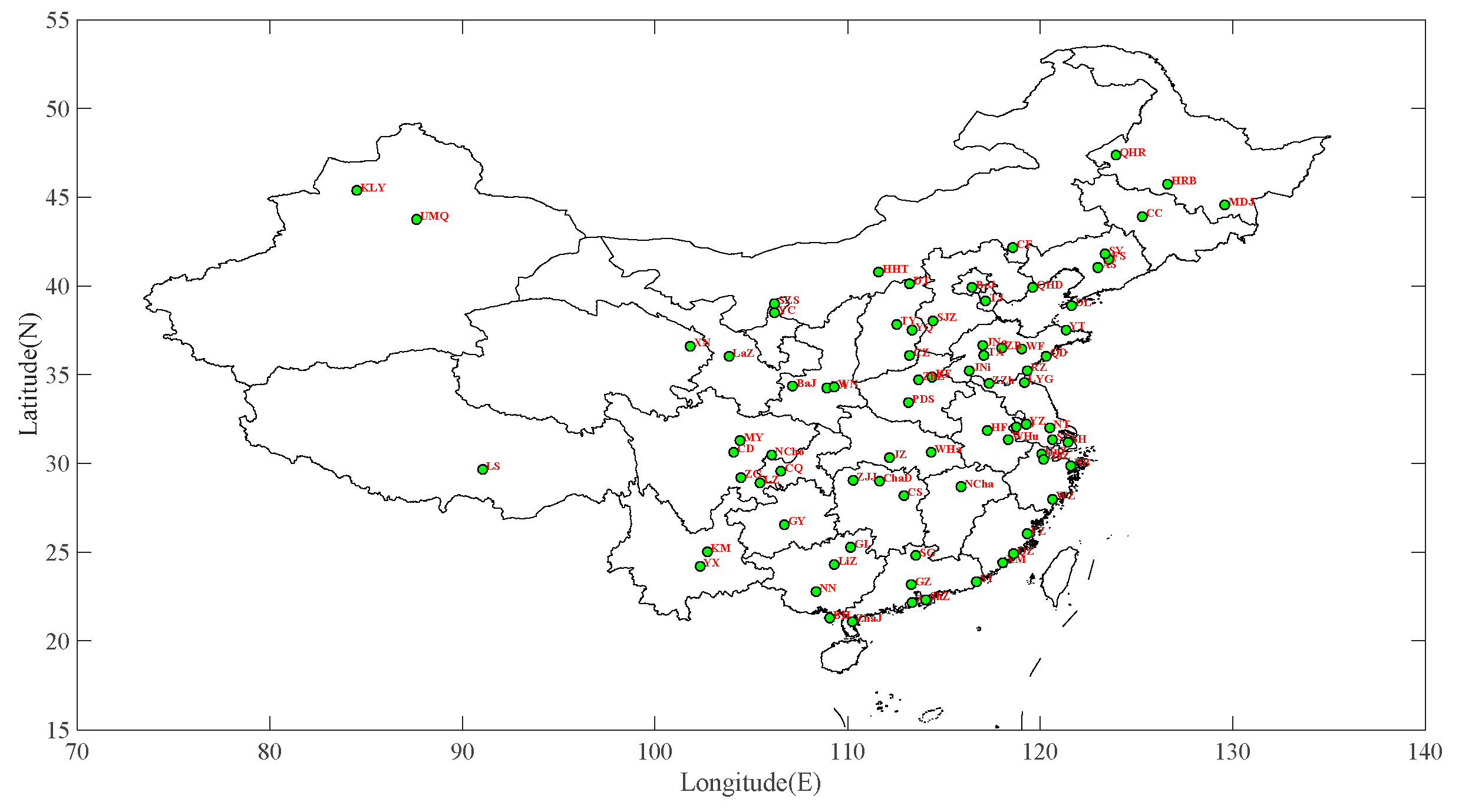
2.1. Study Region and Data

A simulation of ground-level PM_2.5 concentrations was carried out over a grid area of China with a spatial extent between 15° and 55° north latitude and 70° and 140° east longitude (Figure 1). The resolution of grid cells was determined to be 0.5° × 0.5°, which was determined for the convenience of analysis and discussion of results. In order to provide additional insight into the spatial aspects of air pollution across the country, 80 major cities were picked out according to economic development, climate, industrial activity and topography. The majority of the sample cities were distributed in the three most developed area: the Beijing–Tianjin–Hebei Region, the Yangtze River Delta, and the Pearl River Delta. The locations of these monitoring sites are plotted in Figure 1.

The PM_2.5 concentration observations in this paper were collected from the China National Environmental Monitoring Center, from January 2014 to November 2014. The experiments were carried out over two time periods according to climate and topography. The first period was from 5 to 11 November 2014. This noteworthy period coincided with the 21th APEC summit in Beijing. A total of 6385 effective PM_2.5 observations were obtained during the winter period. The second period was from 14 to 20 May 2014. A total of 6298 effective PM_2.5 observations were obtained during the spring period.

2.2. Dynamically Constrained Interpolation Methodology

Previous studies have shown that the DCIM combines dynamical constraints from the numerical model of dynamical processes with statistical information from observations, which can produce dynamically and statistically consistent simulation of the entire study area [21,22]. The observations are interpolated by the dynamic numerical model in the DCIM. Moreover, the interpolated results are optimized iteratively by adjusting the key model parameters through the adjoint method [21,24].

2.2.1. The Dynamic Model

Generally speaking, PM_2.5 varied due to interactions among many processes including emissions (anthropogenic emission and natural dust production), transport (as well as convection-influenced dispersion and dilution), photochemical transformation (new particle speciation and production of secondary PM_2.5), and deposition (dry and wet), with meteorology playing an overarching role [24]. Because of the complexity of the sources and sinks, the general PM_2.5 adjoint model included a rich description of the photochemical oxidant cycle and a chemical mechanism to simulate the formation of secondary PM_2.5. The adjoint method is useful for assimilating the observations to obtain reasonable model parameters and is used widely in meteorology [24,25,26,27,28,29].

However, the adjoint model was significantly difficult to build because of complex chemical mechanisms. To reduce the complexity of the model and achieve the purpose of simulation we took the primary PM_2.5 and secondary PM_2.5 as a whole, calling it the “source and sink term” (SAST) without considering the specifics. Because of the type of observations and the uncertainty of vertical variation, we established a two-dimensional (2D) PM_2.5 CTM in rectangular coordinates as follows:

$$\frac{\partial C}{\partial \mathrm{t}}+u\frac{\partial C}{\partial x}+v\frac{\partial C}{\partial y}=\frac{\partial }{\partial x}\left(A_H\frac{\partial C}{\partial x}\right)+\frac{\partial }{\partial y}\left(A_H\frac{\partial C}{\partial y}\right)+S$$

(1)

$$C(t^0,x,y)=C^0(x,y),$$

(2)

$$\frac{\partial C}{\partial t}=0,\mathrm{on}{\Gamma }^{\mathrm{OUT}}$$

(3)

$$\frac{\partial C}{\partial \overrightarrow{n}}=0,\mathrm{on}{\Gamma }^{\mathrm{OUT}}$$

(4)

Here, C represents the PM_2.5 concentration; u and v are the horizontal wind velocity in the x and y coordinates, respectively; A_H is the horizontal viscosity coefficient; and S is the SAST. The model has initial conditions C⁰ and is subject to constant boundary conditions at the inflow boundary Γ^IN and to no gradient boundary conditions at the outflow boundary Γ^OUT. The detailed numerical scheme for this 2D PM_2.5 CTM is the same as that in [18].

2.2.2. Parameter Optimization by the Adjoint Method

In order to construct the adjoint model, the cost function is defined as

$$J=\frac{1}{2}{\displaystyle {\int }_{\Sigma }K{\left(C-C_{\mathrm{obs}}\right)}^2}\mathrm{d}\sigma$$

(5)

Based on the theory of the Lagrangian multiplier method, the Lagrangian function is defined as

$$L=J+{\displaystyle \int \left\{p\times \left[\frac{\partial C}{\partial \mathrm{t}}+u\frac{\partial C}{\partial x}+v\frac{\partial C}{\partial y}-\frac{\partial }{\partial x}\left(A_H\frac{\partial C}{\partial x}\right)-\frac{\partial }{\partial y}\left(A_H\frac{\partial C}{\partial y}\right)-S\right]\right\}\mathrm{d}\mathsf{\Omega }}$$

(6)

Here Σ is the set of the observations; C and C_obs are the simulated and observed PM_2.5 concentrations, respectively; p denotes the adjoint variable of C; and K is the weighting matrix and theoretically should be the inverse of the observation error covariance matrix. Assuming the errors of the data are uncorrelated and equally weighted, K can be simplified, and in this study K is 1 if observations are available and 0 otherwise.

To let the cost function reach the minimum, we make the first-order derivates of Lagrangian function with respect to all the variables and parameters to be zero:

$$\frac{\partial L}{\partial p}=0,$$

(7)

$$\frac{\partial L}{\partial C}=0,$$

(8)

$$\frac{\partial L}{\partial k}=0,$$

(9)

where k is the key model parameters, which includes initial condition, A_H and S.

From Equation (8), the adjoint model for the 2D PM_2.5 CTM, which governs the evolution of the adjoint variable p, can be obtained. From Equation (9), the gradients of the cost function with respect to the key model parameters A_H and S can be deduced. The detailed description of the adjoint model and gradients can be found in [18]. Based on the gradients obtained from Equation (9), the key model parameters can be optimized using the steepest descent method.

2.2.3. Default Settings of the Dynamical Model

The resolution of grid cells was determined to be 0.5° × 0.5°. There were 81 grid cells in the x direction and 141 cells in the y direction. The integral time step was 600 s. The first studied period coincided exactly with the 21th Asia–Pacifc Economic Cooperation (APEC) summit taking place in Beijing, and this studied period was divided into two parts: the initial simulation period and target simulation period. The initial simulation time was 72 h and from 5 to 7 November 2014. The target simulation time was 96 h and from 8 to 11 November 2014. The second studied period was from 14 to 20 May 2014, and the initial simulation time was 72 h (from 14 to 16 May 2014). The target simulation time was 96 h (from 17 to 20 May 2014).

The initial meteorological fields adopted in our experiments were from NCEP Climate Forecast System (CFS-R/CFSv2) with 0.5° × 0.5° spatial resolution and 1 h temporal resolution. The dynamic model was subject to constant boundary conditions at the inflow boundary and to no gradient boundary conditions at the outflow boundary. According to the new ambient air quality standards announced by China’s Ministry of Environmental Protection (MEP) in 2013, inflow boundary values were fixed as 35.0 µg/m³. The horizontal diffusion coefficient $A_H$ was fixed as 100.0 m²/s. In view of the importance of initial conditions to the simulated results of a dynamic model [21,24,25,26], the initial conditions were obtained by interpolating the observed PM_2.5 using surface spline interpolation [21].

2.2.4. The Process of DCIM

Previous studies have indicated that the DCIM was a feasible and effective method for interpolating the sparse observations for both space and time, which can improve the utilization of these observations [21,24,25,26,27,28,29]. Based on the processes to interpolate the sparse observations using DCIM in [21,24], the processes to simulate the PM_2.5 concentrations at national scale using DCIM in this paper were as follows:

Step 1. Assign the initial guess values to all the model parameters in the dynamic model (i.e., 2D PM_2.5 CTM in this study). Divide observation period into two parts: the initial simulation period and target simulation period.

Step 2. Run the dynamic model in the initial simulation period and acquire the interpolated results.

Step 3. Calculate the cost function and then integrate the adjoint model backward in time to get the adjoint variables.

Step 4. Compute the gradients of the cost function with respect to the key model parameters (spatially varying initial conditions and S in this study).

Step 5. Adjust the key model parameters utilizing the steepest descent method, and update the values of the key model parameters in the dynamic model.

Step 6. Check whether the cost function has satisfied the requirements of minimization. If the minimization requirement is satisfied, then terminate the iteration and go to Step 7; otherwise, return to Step 2.

Step 7. Set the interpolated PM_2.5 concentrations at the last time-step obtained using the DCIM as the initial condition. Run the dynamic model with the optimized key model parameters to simulate the PM_2.5 concentrations over the following two hours.

Step 8. The initial time of the initial simulation period is longer by two hours. Take the interpolated results at this initial time as initial condition and assign the initial guess values to all the model parameters. Repeat Step 2 through Step 7 to simulate the PM_2.5 concentrations over the next two hours.

Repeat Step 2 through Step 8, until all the PM_2.5 concentrations in the target simulation period are simulated.

In this study, the sparsely observed PM_2.5 concentrations were interpolated for space and time to perform the simulations following the aforementioned processes. We focus on the simulation results in the target period. When the DCIM was implemented, the key model parameters, including spatially varying initial conditions and SAST, were adjusted synchronously while the other model parameters remained constant.

2.3. The OPF Method Based on Chebyshev Basis Functions

The OPF method based on Chebyshev basis functions was an effective method for reconstructing the PM_2.5 fields accurately in the central and southern regions of China [20]. In our study, the OPF method based on Chebyshev basis functions (COPF) followed the definitions shown in [20]. Let $x_i$ be the points on $x$ axis ($i=1,2\cdots ,I$). The Chebyshev polynomials in the $x$ direction are

$$\begin{array}{l}{\Phi }_{\mathrm{o}}{(x}_i)=1,\\ {\Phi }_1{(x}_i{)=x}_i-P_{1,0}{\Phi }_0{(x}_i),\\ {\Phi }_2{(x}_i{)=x}_i{}^2{P}_{2,1}{\Phi }_1{(x}_i)-P_{2,0}{\Phi }_0{(x}_i),\\ \dots \\ {\Phi }_k{(x}_i{)=x}_i{}^k-P_{k,k-1}{\Phi }_{k-1}{(x}_i)-P_{k,k-2}{\Phi }_{k-2}{(x}_i)-\dots -P_{2,0}{\Phi }_0{(x}_i),\end{array}$$

(10)

where $k$ is the order of the polynomials in the $x$ direction, ${\Phi }_{\mathrm{o}}{(x}_i)$, ${\Phi }_1{(x}_i)$ …${\Phi }_k{(x}_i)$ are Chebyshev polynomials from order zero to k. $P$ is the coefficient of Chebyshev polynomials and defined as

$$P_{k,l}=\frac{{\displaystyle \sum _{i=1}^I{x}_i^k{\Phi }_l{(x}_i)}}{{\displaystyle \sum _{i=1}^I{\Phi }_l^2{(x}_i)}},$$

(11)

where $P_{k,l}$ is the l-th coefficient of the $k$-order polynomial. The Chebyshev polynomials in the $y$ direction also follow the above definition.

PM_2.5 data sets are denoted by $\left(x_i,y_i,z_i\right),i=1,2\cdots ,I$, where $x$ is a rectangular coordinate converted from longitudes based on the stereographic map projection; $y$ is rectangular coordinate converted from latitudes based on the stereographic map projection, $z$ is the PM_2.5 observation; and $I$ is the total number of the data. The PM_2.5 observations ${Z(x}_i{,y}_i)$ can be stated as

$$\tilde{Z}(x_i,y_i)={\displaystyle \sum _{k=0}^{K_0}{\displaystyle \sum _{\mathrm{s}=0}^{S_0}{A}_{k,\mathrm{s}}{\Phi }_k{(x}_i{)\varsigma }_{\mathrm{s}}{(y}_i)}},$$

(12)

where $i=1,2\cdots ,I$, $k$ and $s$ are the orders of polynomials for the $x$ and $y$ directions, respectively. K₀ and S₀ are the corresponding cutoff orders. $A_{k,\mathrm{s}}$ are expansion coefficients. ${\Phi }_k{(x}_i)$ is the k-order Chebyshev orthogonal polynomial in the $x$ direction. and ${\varsigma }_{\mathrm{s}}{(y}_i)$ is the s-order Chebyshev orthogonal polynomial in the $y$ direction.

Based on the least-square method, the expansion coefficients can be solved as

$$A_{k,\mathrm{s}}=\frac{{\displaystyle \sum _{i=1}^I{\displaystyle \sum _{j=1}^I{Z(x}_i{,y}_i{)\Phi }_k{(x}_i{)\varsigma }_{\mathrm{s}}{(y}_i)}}}{{\displaystyle \sum _{i=1}^I{\Phi }_k^2{(x}_i){\displaystyle \sum _{j=1}^I{\varsigma }_{\mathrm{s}}^2{(y}_i)}}}.$$

(13)

3. Results and Analysis

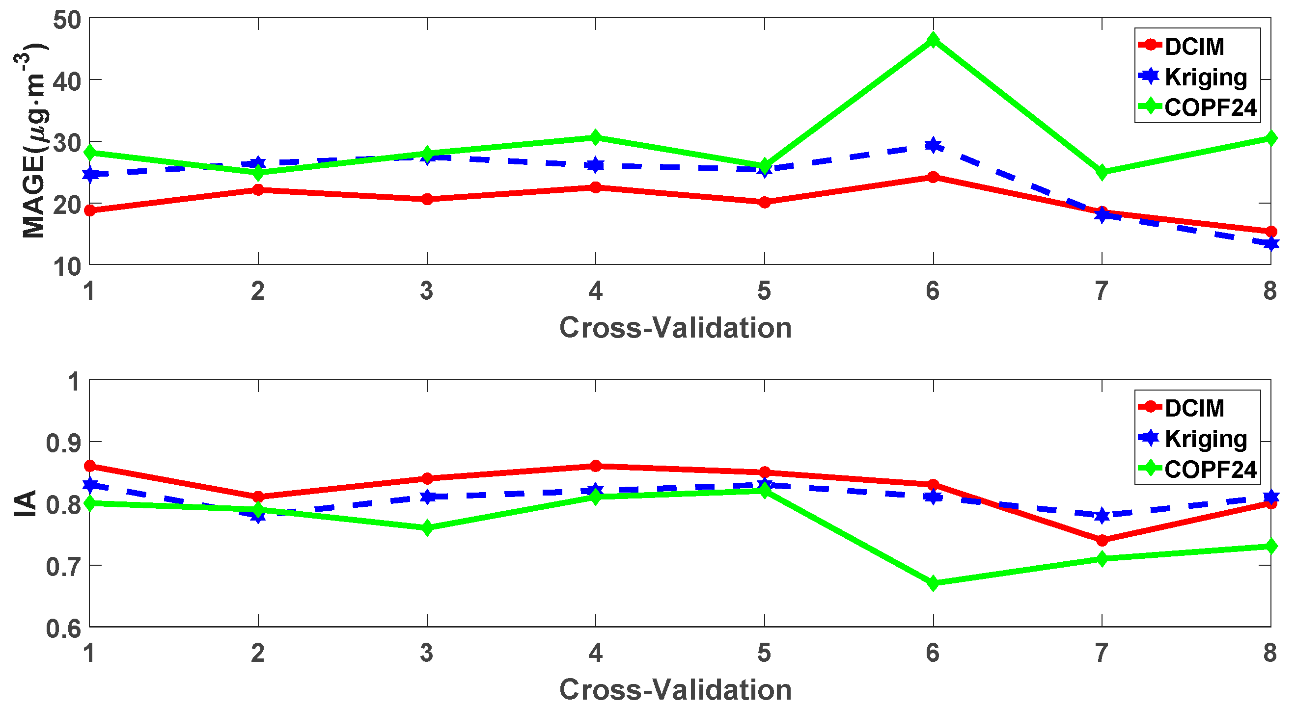
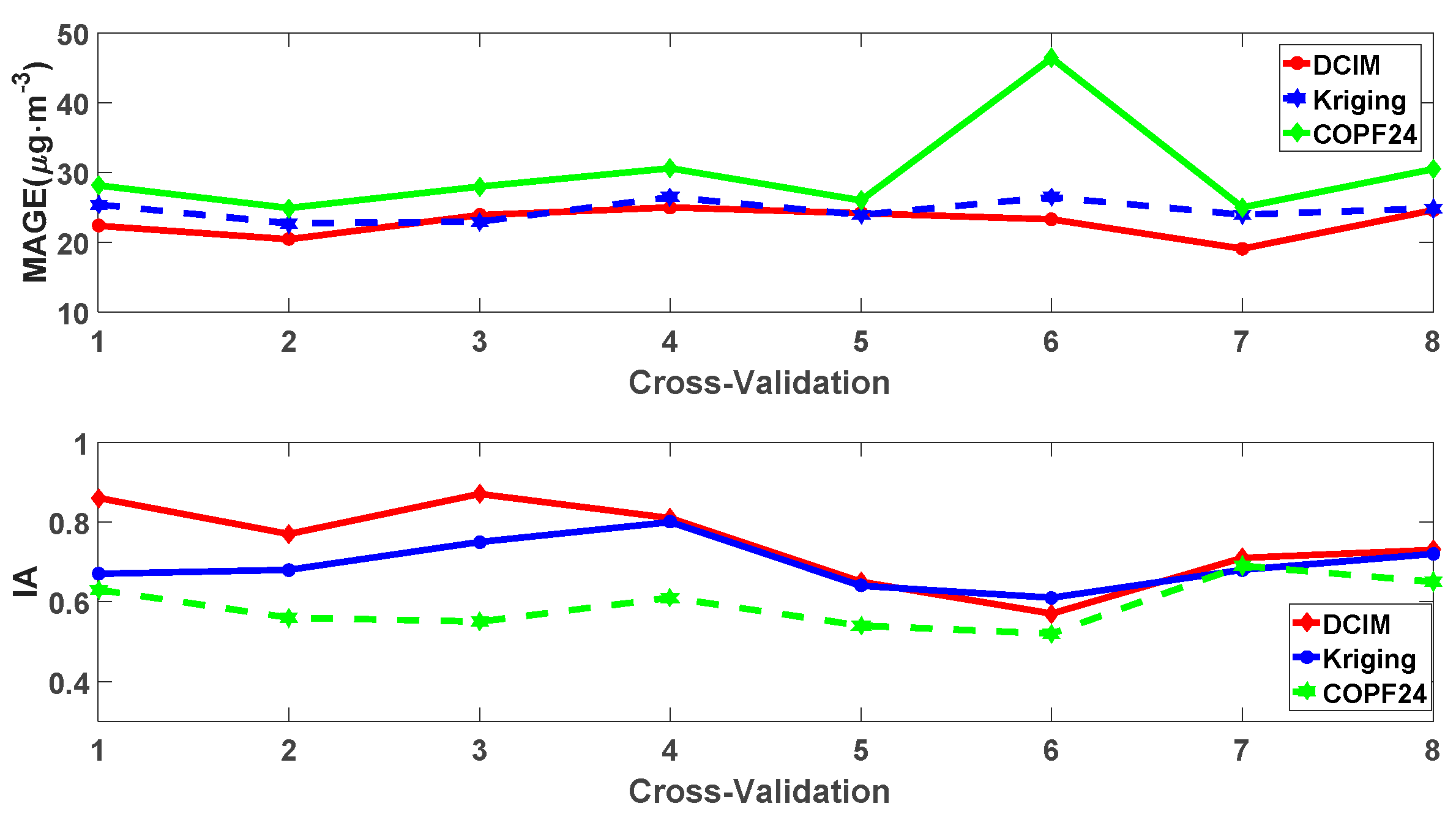
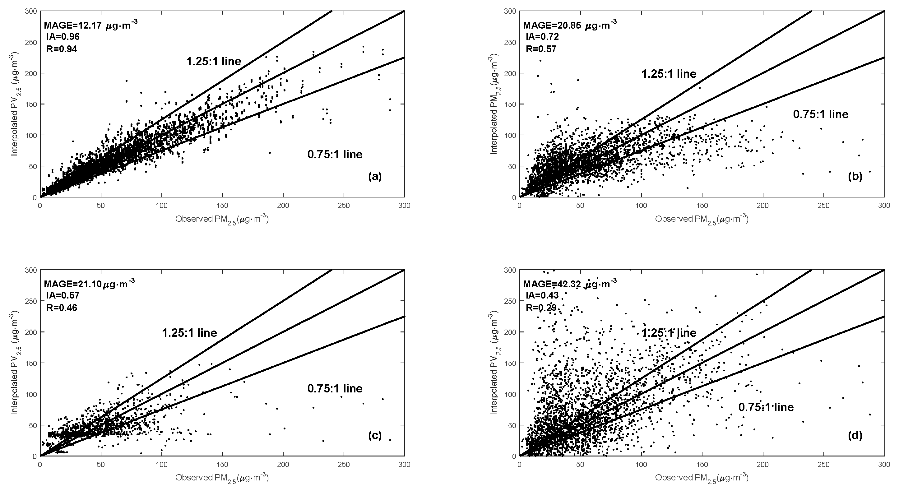
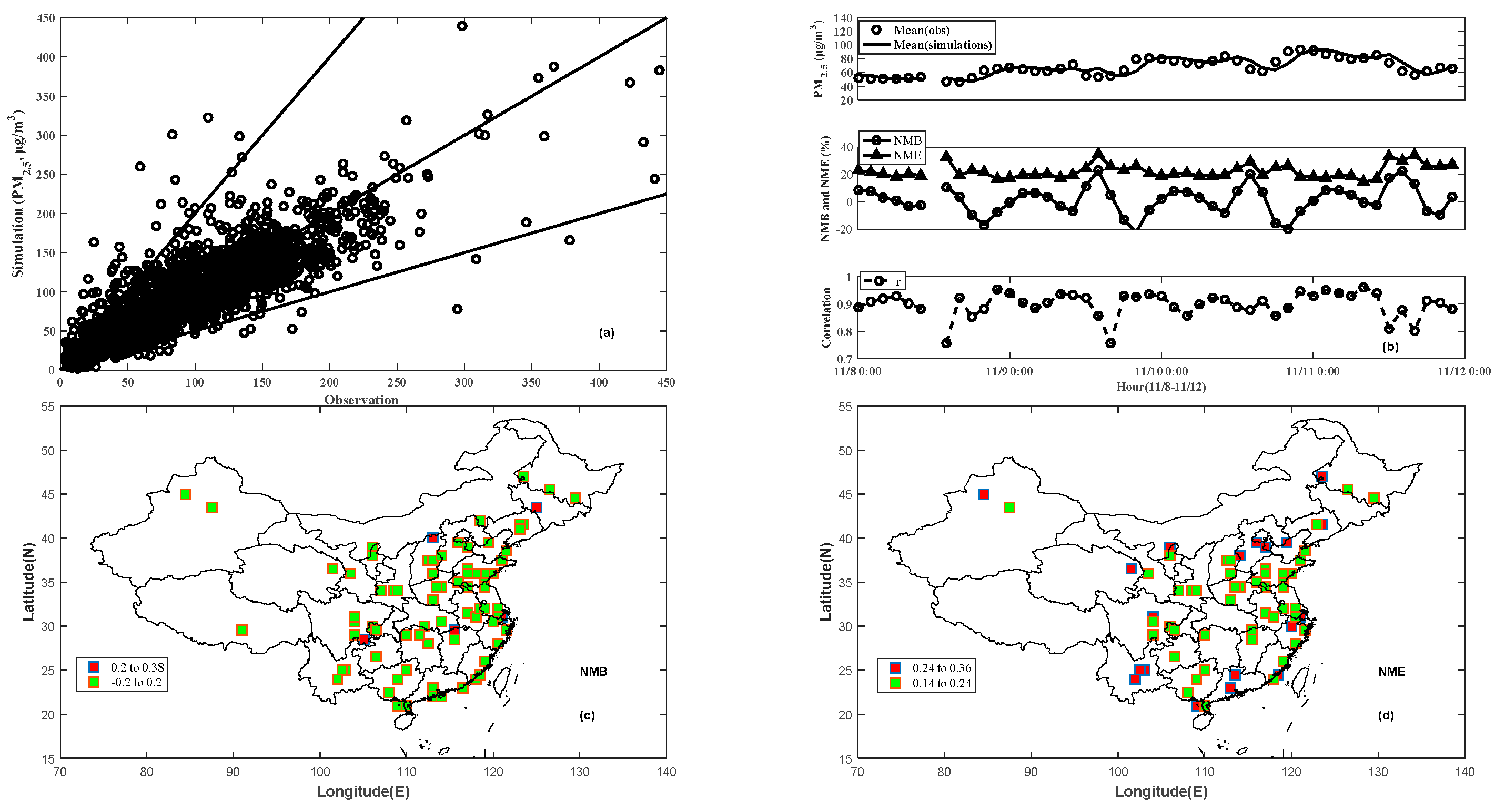
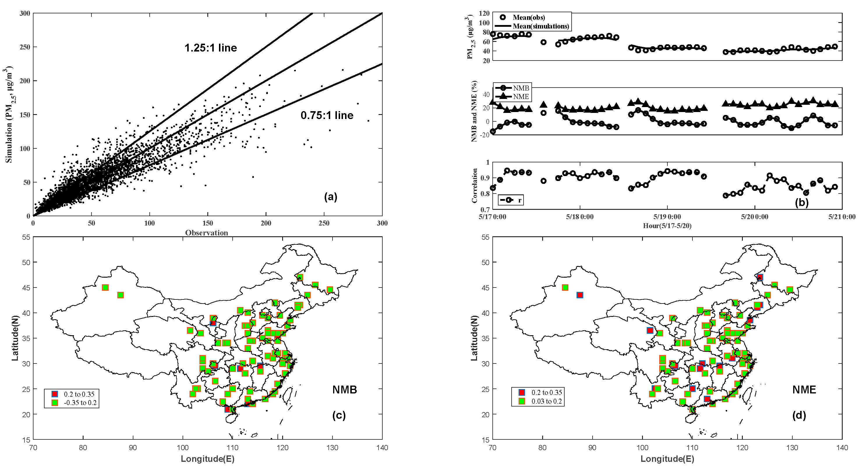
3.1. Verification and Evaluation of DCIM

In this part, the 8-fold cross-validation technique was applied to evaluate the simulation power of the DCIM [16,24]. The 80 sampled cities were randomly divided into 8 folds. Seven folds were selected as the training set and labeled as interpolated samples, the datasets of which were interpolated to obtain the corresponding simulations. The other fold was employed as the validation set, the datasets of which were not used for interpolation but only for verification and labeled as checked samples. This process was repeated 8 times until every fold was tested.

Evaluation indices, including the mean absolute gross estimation error (MAGE), the mean normalized gross estimation error (MNGE), the correlation coefficient (R), and the index of agreement (IA), were adopted to evaluate the performance of the DCIM. The correlation coefficient indicates the correlation between simulations and observations. IA is a dimensionless indicator of accuracy between zero and one, which describes how well simulations and observations agree. The closer the values approach one, the more accurate the simulation. Their specific definitions, shown as follows, were calculated by the value of simulation and observations:

$$\mathrm{MAGE}=\frac{1}{N}{\displaystyle \sum _{i=1}^N\left|P_i-O_i\right|}$$

(14)

$$\mathrm{MNGE}=\frac{1}{N}{\displaystyle \sum _{i=1}^N\left[\left(\left|P_i-O_i\right|\right)/O_i\right]}$$

(15)

$$\mathrm{R}=\frac{{\displaystyle \sum _{i=1}^N\left(P_i-\overline{P}\right)(O_i-\overline{O})}}{\sqrt{{\displaystyle \sum _{i=1}^N{(P_i-\overline{P})}^2{\displaystyle \sum _{i=1}^N{(O_i-\overline{O})}^2}}}}$$

(16)

$$\mathrm{IA}=\frac{1-{\displaystyle \sum _{i=1}^N{\left(P_i-O_i\right)}^2}}{{\displaystyle \sum _{i=1}^N{\left(\left|P_i-\overline{O}\right|+\left|O_i-\overline{O}\right|\right)}^2}}$$

(17)

where N was the number of observations; P and O were the simulated PM_2.5 concentrations and observations; and $\overline{P}$ and $\overline{O}$ were mean simulations and mean observations, respectively. For the DCIM method, we tried the evaluation procedure 8 times to check potential bias from using the result of a single time. Therefore a total of eight groups of experiments, named as PE_1–PE_8, were implemented.

The COPF method and kriging interpolation were used for comparison. Reference to the work in [20], the semivariogram model was chosen as a spherical semivariogram model for the kriging interpolation in our study. The range and sill were respectively fixed to 10° and 1°. Due to the limited numbers of available observations, the range of polynomial orders in the x and y directions were limited to 8 in the COPF method. PM_2.5 distributions were calculated 81 times (polynomial orders of x and y directions each increased from 0 to 8) in the cross-validation. The optimal orders were found when the order combinations reached the minimal average MAGEs and IA of the verification cities.

The 8-fold cross-validation experiments were implemented in the first target discussion period from November 8 to 11, 2014). For the COPF, all the combinations of k and s (polynomial orders of x and y directions) were tested first. The MAGEs and IA arrived at the minimum when s and k were set to 2 and 4, respectively. In this way, the optimal degree of COPF was found, and we denoted it by COPF24. The DCIM simulations were compared with the simulations obtained from kriging and COPF24.

The results of the 8-fold DCIM cross-validation experiments on November 8–11, 2014, were displayed in

Table 1. Simulation Error for the 8-fold cross-validation DCIM experiments at the initial and final iteration steps of DCIM experiments on 8–11 November 2014.

Expt	K1 a (µg/m3)		K2 a		K3 a (µg/m3)		K4 a
	Initial	Final	Initial (%)	Final (%)	Initial	Final	Initial (%)	Final (%)
PE_1	41.23	11.66	61.89	22.35	43.31	23.86	65.72	57.16
PE_2	41.79	12.62	61.89	22.47	39.31	26.01	65.64	59.26
PE_3	39.91	10.21	63.05	24.58	52.61	26.73	57.34	50.10
PE_4	42.76	10.60	59.80	23.26	32.29	22.04	80.78	70.19
PE_5	40.02	10.40	64.06	24.86	46.77	23.86	49.97	41.13
PE_6	42.51	11.60	63.72	24.75	39.47	24.20	47.03	43.62
PE_7	43.56	13.59	64.05	24.68	19.50	17.66	60.97	57.35
PE_8	45.33	16.01	59.96	23.45	13.90	12.41	79.47	67.11

K1 ^a is MAGEs between the observations and the corresponding simulated PM_2.5 in interpolated samples. K2 ^a is MNGEs between the observations and the corresponding simulated PM_2.5 in interpolated samples. K3 ^a is MAGEs between the observations and the corresponding simulated PM_2.5 in checked samples. K4 ^a is MNGEs between the observations and the corresponding simulated PM_2.5 in checked samples_.

and

Table 2. Correlation coefficient and index of agreement for the 8-fold cross-validation DCIM experiments on 8–11 November 2014.

Expt	K1 a	K2 a	K3 a	K4 a
PE_1	0.97	0.95	0.88	0.77
PE_2	0.96	0.93	0.82	0.70
PE_3	0.97	0.96	0.85	0.73
PE_4	0.98	0.96	0.88	0.78
PE_5	0.96	0.93	0.87	0.76
PE_6	0.96	0.93	0.84	0.70
PE_7	0.96	0.94	0.79	0.69
PE_8	0.96	0.94	0.83	0.71

K1 ^a is the index of agreement in interpolated samples. K2 ^a is the correlation coefficient in interpolated samples. K3 ^a is the index of agreement in checked samples. K4 ^a is the correlation coefficient in checked samples.

(Estimation errors for the 8-fold cross-validation DCIM experiments). For the interpolated samples, MAGEs between the observations and the corresponding 8-fold cross-validation DCIM simulations dropped at least 60.89%, which was reduced from 45.33 µg/m³ to 16.01 µg/m³. The corresponding MNGEs decreased by 60.89%, which occurred in PE_8 (see Table 1). Furthermore, values of R (from 0.93 to 0.96) and IA (from 0.96 to 0.98) showed significant accuracy and correlation between interpolated observations and the corresponding 8-fold cross-validation DCIM simulations. For the checked samples, the largest drop in the MAGEs and MNGEs between the observations and the final 8-fold cross-validation DCIM simulations were 49.19% and 17.69%, respectively. Compared with the results of the interpolated samples, the discrepancies between the simulations and the observations were slightly large, but all much less than those at the initial iteration step. Meanwhile, the values of R (from 0.69 to 0.78) and IA (from 0.79 to 0.88) indicated a reasonable range of the national-scale DCIM simulations.

The comparison results of different methods were illustrated in Figure 2 (Interpolation errors in checked samples of different methods for the 8-fold cross-validation experiments) and Figure 3 (Scatter plots and performance of different methods for the 8-fold cross-validation experiments). As shown in Figure 2, the MAGEs and IA of the DCIM were lower than those of kriging interpolation and COPF24 in most of the cross-validation processes except for PE_7 and PE_8. The interpolation errors of kriging interpolation were larger than those of the COPF24 in most of the cross-validation processes except for PE_8. As illustrated in Figure 3, the averaged MAGEs of the DCIM, kriging and COPF24 were 21.93, 24.15 and 25.92 μg·m⁻³, respectively. The averaged IAs in checked samples of the DCIM, kriging and COPF24 were 0.80, 0.79 and 0.51, respectively. In summary, multiple runs produced similar results, with little difference.

Figure 3 illustrates the scatterplot that compares the performance of different methods for the 8-fold cross-validation experiments on 8–11 November 2014. The 1.25:1, 1:1 and 0.75:1 lines are shown for reference. According to the validation scatter plots shown in Figure 3, the DCIM captured 72.91% of the observations in the checked samples within the 1.25:1 line and the 0.75:1 line, which verified the usefulness of the DCIM on PM_2.5 simulations. The kriging interpolation and the COPF24 captured 72.83 and 69.60% of the observations, respectively. Meanwhile, the DCIM captured 78.89% of the observations in the interpolation samples within the 1.25:1 line and the 0.75:1 line. By comparison with the results from the kriging interpolation and the COPF24, the DCIM clearly had the highest accuracy. The 8-fold cross-validation DCIM simulations of all the sampled cities in target simulation period were more consistent with the observations. The COPF method performed worse than the DCIM and kriging in national-scale simulations during this period.

The 8-fold cross-validation experiments were implemented in the second target discussion period (17–20 May 2014). In this period, the COPF achieved the minimum errors when s and k were set to 2 and 4. The results of COPF24 were used for comparison. The comparison results of different methods were illustrated in Figure 4 (Interpolation errors of different methods for the 8-fold cross-validation experiments) and Figure 5 (Scatter plots and performance of different methods for the 8-fold cross-validation experiments). The DCIM simulations of the checked samples were more accurate than those of kriging and COPF24, with less mean MANGEs and IAs for the 8-fold cross-validation experiments. The DCIM captured 77.59% of the observations in the checked samples within the 1.25:1 line and the 0.75:1 line, which verified the usefulness of the DCIM on PM_2.5 simulations. The kriging interpolation and COPF24 captured 82.78 and 77.59% of the observations, respectively. Meanwhile, the DCIM captured 88.34% of the observations in the interpolation samples within the 1.25:1 line and the 0.75:1 line. On the whole, the result demonstrated that the DCIM can be deemed more effective in national-scaled PM_2.5 simulations, compared with the kriging interpolation and COPF method.

3.2. Performance of the DCIM

In the process of data analysis, it had been found that the checked samples showed a larger simulation error than the interpolated samples. That was to say, in DCIM, interpolated all the observations may improve the simulation accuracy. In order to further validate the simulation results, all the observations were interpolated in DCIM to simulate concentrations of PM_2.5 with the strategy stated in Section 2.2.3. Simulation errors analysis of the target simulation period was adopted to further investigate DCIM performance.

For the first target period (From 8 to 11 November), the MAGEs between the observations and the DCIM simulations were decreased from 41.48 µg/m³ to 12.54 µg/m³, which was a decline of 69.77%. The corresponding MNGEs were decreased from 62.35% to 25.31%, which was down 59.41%. Furthermore, the values of R (0.91) and IA (0.95) indicate that DCIM is a feasible simulation method and high in accuracy. For the DCIM performance evaluation, regression statistics along with the normalized mean bias (NMB), and another measure of error, normalized mean error (NME) [26], were further calculated. The mean value of NMB and NME were 0.26% and 21.04%, respectively. Furthermore, the mean value of all the observations was 68.73 µg/m³, and the mean value of the simulated results was 68.34 µg/m³. Figure 6a illustrated the scatterplot to compare the observations and the DCIM simulations visually. The 1.25:1, 1:1 and 0.75:1 lines were shown for reference. For 90.83% of the observations, the ratio was between 0.75 and 1.25, which verified the usefulness of the DCIM on PM_2.5 simulations.

On the other hand, it should be noted that the national-scale simulations of PM_2.5 in China were almost always underestimated in high PM_2.5 concentration range. This issue will be further discussed in Section 4. However, the correlation coefficient (0.94) and IA (0.96) between the observations and simulated results indicated the DCIM showed a reasonable scope of underestimation. Meanwhile, Figure 6b had shown the usefulness of the DCIM in time series analysis and simulation. The values of mean, NMB, NME and correlation coefficients were calculated (spatial averages) and plotted as a two-hour time series (Figure 6b).

As can be seen, the mean values of observations and simulated results were almost equal and had the same time-varying trend. The NMB values ranged from–17.99% to 20.21%, the NME values were approximate to 19.50%, and correlation coefficients ranged from 0.89 to 0.97, which proved that the DCIM was stable with time. Figure 6c,d showed the spatial distributions of the NMB and NME between the observations and the simulation results. The DCIM simulated PM_2.5 well in most areas (85.64%), where the NMB value was less than 0.20 and the NME value was also less than 0.20.

To further verify the simulation ability, the DCIM was implemented in the spring, from 14 to 20 May 2014. The initial simulation period was from 14 to 16 May. And the target simulation period was from 17 to 20 May. All the observations over the initial simulation period were interpolated to simulate PM_2.5 concentrations from 17 to 20 May, according to the strategy stated in Section 2.2.3. Simulation errors analysis of the target simulation period was adopted to further investigate DCIM performance. For the performance evaluation, regression statistics along with two measure of bias (the mean bias (MB) and the normalized mean bias (NMB)), and two measures of error (the root mean square error (RMSE) and normalized mean error (NME)), were calculated. The mean value of MB and RMSE were −0.07 µg/m³ and 18.73 µg/m³ respectively, and those for NMB and NME were −0.12% and 20.94%, respectively. Furthermore, the correlation coefficient between the observations and simulated results was 0.89.

Figure 7a illustrated the scatterplot to compare the observations and the DCIM simulations visually. The 1.25:1, 1:1 and 0.75:1 lines were shown for reference. For 75.63% of the observations, the ratio was between 0.75 and 1.25. In order to investigate the performance of DCIM over time, the values of mean, NMB, NME and correlation coefficients were calculated (spatial averages) and plotted as a time series (Figure 7b). As can be seen, the mean values of observations and the simulated results were almost equal and have the same time-varying trend. The NMB values ranged from −14.37% to 16.90%. The NME values ranged from 14.82% to 24.56%, which proved that the DCIM was steady during the time. Spatially, the DCIM estimated observed PM_2.5 well in most areas (79.35%) where the NMB value was less than 0.2 and the NME value was also less than 0.2 (Figure 7c,d).

To sum up, the DCIM provided effective dynamic information compared with kriging and COPF. First, the time series analysis of the simulation values using mean, NMB, NME and correlation coefficients showed that the DCIM can achieve a more accurate real-time simulation, which the dynamically unconstrained interpolation techniques were unable to achieve. Second, the DCIM can also give the characteristics of the spatiotemporal variation parameters during the target simulation periods, which contributed to the existing relevant research in China to a certain extent.

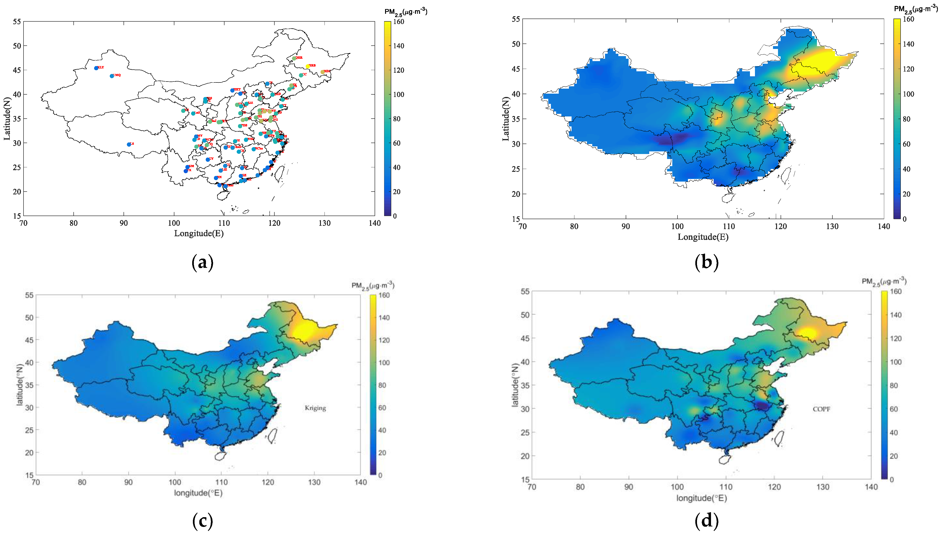
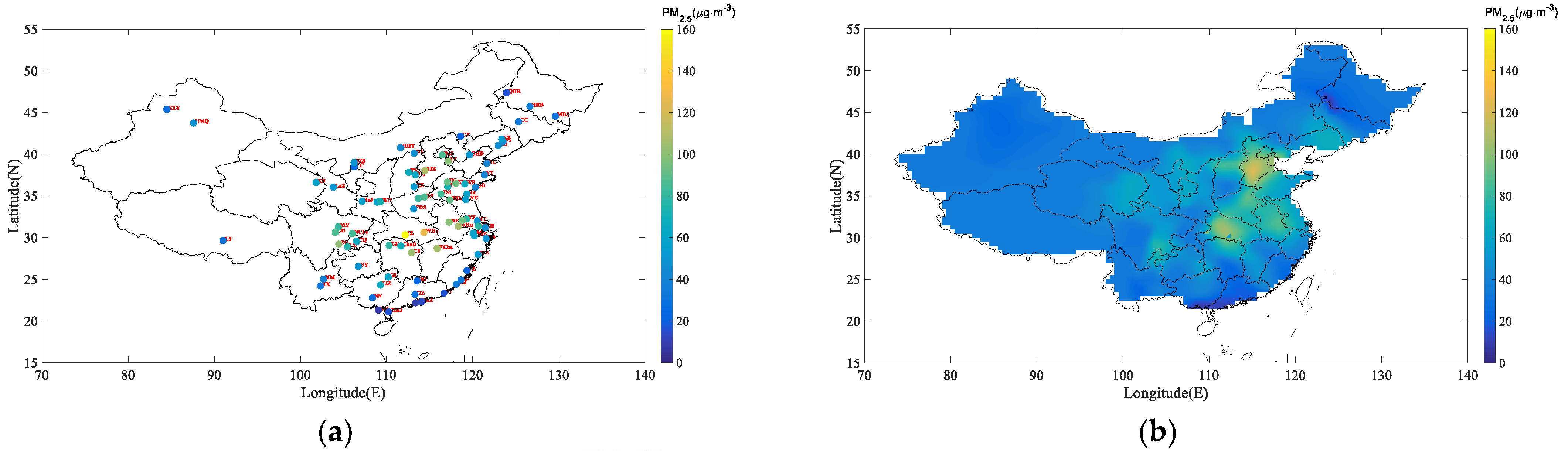
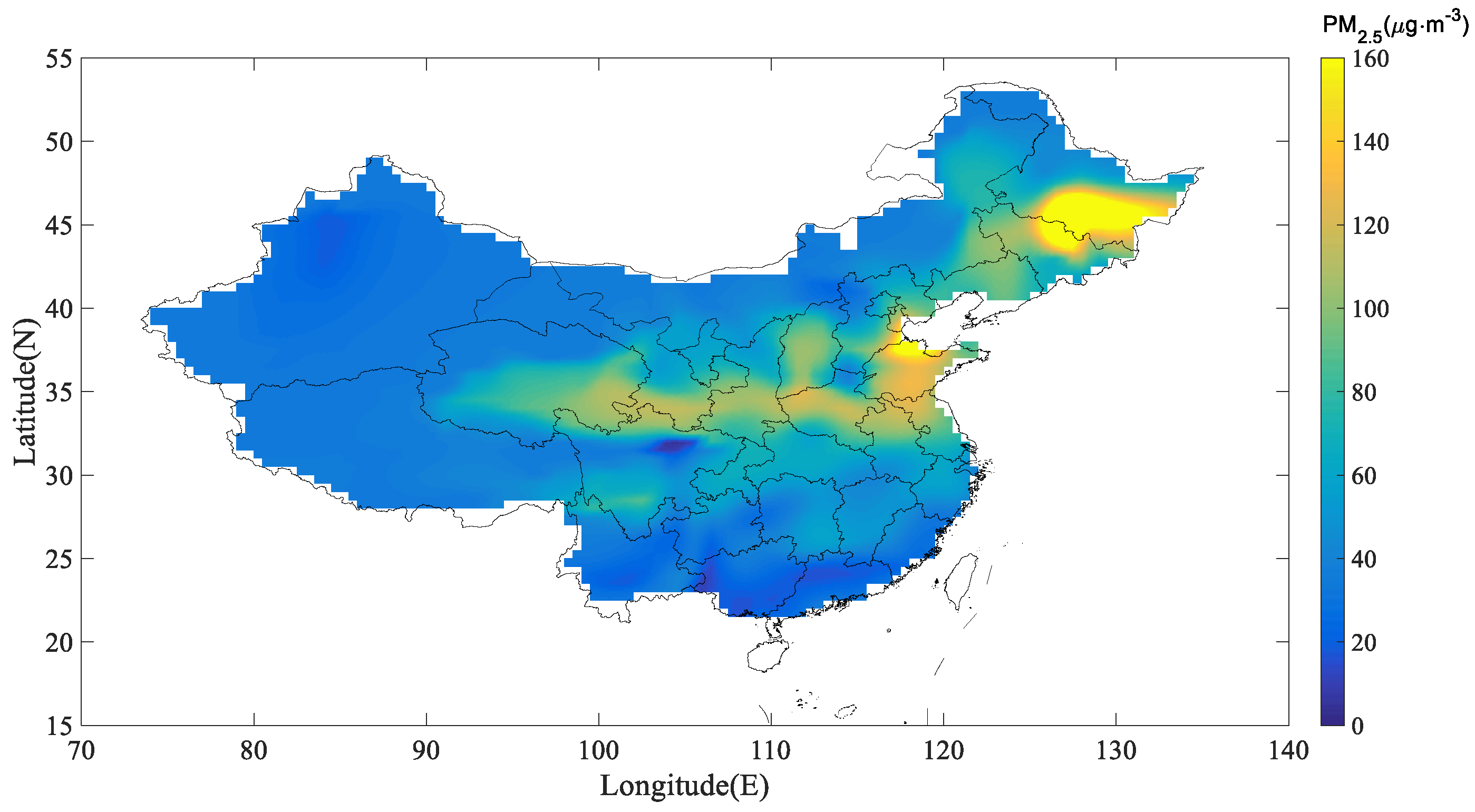
3.3. Mapping of the Mean PM_2.5 Simulations

The mean observations of the 80 sample cities and mean distributions of PM_2.5 on 8–11 November 2014 were mapped in Figure 8. The mean distributions of DCIM, kriging and COPF showed similar distribution with the mean observations map. The DCIM results presented a smoother pattern with a smaller MAGE than the results from the other methods did. As can be seen from the DCIM results, the levels of PM_2.5 simulations were higher in the northern region than in the southern. Shandong and Jiangsu provinces presented higher PM_2.5 concentrations, which was in conformity with industrial development. Guangdong and Fujian provinces presented lower PM_2.5 concentrations due to the low levels of anthropogenic emissions and favorable meteorological conditions for atmospheric dispersion [10]. Meanwhile, heavily polluted regions were identified in North and Northeast China, PM_2.5 concentrations of which rose to 120–160 µg/m³ during the target simulation period. Compared with the MODIS-derived seasonal mean 1 km-resolution PM_2.5 maps averaged over the winter period 2000–2018 as shown in [30], the DCIM results showed similar spatial distribution but presented a higher level of PM_2.5 concentrations in Northeast China. One major reason for the higher level might be the serious pollution from coal combustion in winter, as reported in a previous study [26]. Adverse weather conditions (i.e., long, dry winter that require indoor heating) further intensified the haze epidemic in northern cities. Another reason might be the atmospheric conditions of aerosols, caused by stagnant weather, with a weak wind and planetary boundary layer [31]. It was noteworthy that air quality in Beijing and Hebei (60–80 µg/m³) was much improved, which benefited from the introduction of an emergency emissions-reduction strategy during the Asia–Pacific Economic Cooperation (APEC) summit in November.

The mean observations of the 80 sample cities and mean distributions of PM_2.5 during 17 May to 20 May 2014 were mapped in Figure 9. In detail, the DCIM, kriging interpolation and COPF obtained similar national-scale mean distributions with the mean observations map during 17 May to 20 May 2014. With smaller errors, the DCIM presented smoother pattern. Figure 9 illustrated that the mean values of PM_2.5 concentrations were much larger in the middle China, where the emission of PM_2.5 concentrations was enormous. And the mean values were smaller in southeast China, where the precipitation was rich. Compared with the research results in the same period in [18], similar spatial distribution of PM_2.5 concentrations indicated the rationality of the DCIM.

4. Discussions and Conclusions

This study introduced the PM_2.5 transport model based on the adjoint data assimilation to interpolate the sparse observations for simulating the hourly average PM_2.5 concentrations two hours in advance and national-scale spatial distribution of PM_2.5 concentrations in China. From the perspective of interpolation accuracy and effect, this study selected kriging interpolation and COPF, which had been proved to have high PM_2.5 simulation accuracy for comparative analysis.

Comparison between final interpolated values and observations showed that the DCIM was better for national-scale simulation than kriging and COPF during the discussion periods. More importantly, the spatiotemporal variation of the simulated results was physically reasonable (see Figure 6 and Figure 7). Our DCIM results showed a good correlation coefficient and index of agreement, which indicated the PM_2.5 simulations of the analysis period were highly spatially correlated. The mean distributions of DCIM showed similar distribution with that of kriging and COPF. And the DCIM presented smoother reasonable pattern with smaller simulation errors than the other methods. Though seasonal high levels of PM_2.5 concentrations during the analysis period were often recognized to bring significant biases, the final DCIM results in this study presented a relatively high simulation accuracy, which indicated its conceivable application for providing insights into policies to mitigate air pollution in China.

Previous studies had shown that mapping the distribution of PM_2.5 concentration in China faced many challenges because of the wide geographical range, complex terrain and sparse observations from unevenly distributed systematic ground-level monitoring stations [12]. For that reason, the DCIM was adopted to improve utilization of the sparsely observed PM_2.5 concentrations for both space and time [21]. Due to the rigorous mathematical basis and mature development, the transport model was chosen as the dynamical model among numerous models. This article sought to investigate the DCIM performance in the spatiotemporal simulation patterns of PM_2.5 concentrations over China utilizing ground-level observations.

In addition, the PM_2.5 transport model, which provided the dynamic constrains in the DCIM, had been proved to be a good solution in simulating national-scale ground-level PM_2.5 in [25,26]. This adjoint model was easy to implement and had high practical operational performance, which effectively made up for the simulated errors caused by sparse observations. Moreover, a benefit from the adjoint data assimilation, the major parameter estimation can be obtained from the iterative optimization. The ability to provide dynamic information from the final DCIM results cannot be matched by other traditional interpolation methods. Therefore, the final simulations from the DCIM in this study were close to the observed values, which can be accepted as an effective research program of the PM_2.5 distribution and transport.

There were still some limitations to the approach used in this study. On one hand, we tended to underestimate our simulations and such underestimation mostly occurred when the measured ground-level PM_2.5 concentrations were high. In view of the seasonal emission effect in the analysis period, this underestimation may be mostly because of the coal-based industries in north such as coal-fired power plants, iron and steel manufacturing [17]. On the other hand, the uneven sampling distribution of the monitor and limited PM_2.5 measurements may not be able to make a relatively accurate simulation of the spatial concentration. For the target simulation periods in winter, the sparse PM_2.5 measurements in a highly polluted region have a certain degree of influence on the interpolated distribution accuracy and rationality. Therefore, three new cities in the North China Plain (Jinlin, Dandong and Fuxin) were added to the sampled cities. The observations of the new cities were interpolated in the DCIM for the mean distributions of PM_2.5 on 8–11 November 2014, and the new mean distribution of PM_2.5 were mapped in Figure 10. Compared with the mean distribution of PM_2.5 in Figure 8, the new pattern presented was smoother in the North China Plain. In a highly polluted region, the spatial distribution of PM_2.5 would be improved by adding the right amount of the observations in the DCIM experiments. The bias between the simulations and the observations will be reduced with the gradually increasing number of monitoring sites in China and available PM_2.5 measurements.

In addition, it is necessary to indicate that some aspects related to data assimilation and the dynamic model developments are restricted in this study, which should be further improved in future studies. Admittedly, for large-scale regions, the sparse PM_2.5 measurements in a highly polluted region have a certain degree of influence on the interpolated distribution accuracy and rationality. Adding the right amount of the observations can improve this situation. Only using ground-level observations may result in relatively large observational errors in assimilation and independent verification. In future studies, the contemporaneous satellite observations of PM_2.5 will be needed to supplement the data information and provide a further quality check.

Despite the potential application of the spatial interpolation for solving the PM_2.5 studies with sparse data, the simulation of PM_2.5 concentrations involved a large number of dynamic factors. We therefore applied the dynamically constrained interpolation method to give a better representation of the national-scaled PM_2.5 simulations. Overall, compared with the kriging interpolation and COPF, the DCIM was promising for providing reasonable information for the spatiotemporal simulations of PM_2.5 variation in large geographical regions. In order to obtain more accurate spatial distribution in large-scale region we will continue to improve the details of the DCIM.

References

1. Duan, F.K.; He, K.B.; Ma, Y.L.; Yang, F.M.; Yu, X.C.; Cadle, S.H.; Chan, T.; Mulawa, P.A. Concentration and chemical characteristics of PM2.5 in Beijing, China: 2001–2002. Sci. Total Environ. 2006, 355, 264–275. [Google Scholar] [CrossRef]
2. Han, B.; Zhang, R.; Yang, W.; Bai, Z.P.; Ma, Z.Q.; Zhang, W.J. Heavy haze episodes in Beijing during January 2013: Inorganic ion chemistry and source analysis using highly time-resolved measurements from an urban site. Sci. Total Environ. 2016, 544, 319–329. [Google Scholar] [CrossRef]
3. Chang, H.H.; Hu, X.; Liu, Y. Calibrating MODIS aerosol optical depth for predicting daily PM2.5 concentrations via statistical downscaling. J. Expo. Sci. Environ. Epidemiol. 2014, 24, 198–404. [Google Scholar] [CrossRef] [Green Version]
4. Sun, Y.L.; Wang, Z.F.; Fu, P.Q.; Yang, T.; Jiang, Q.; Dong, H.B.; Li, J.J.; Jia, J.J. Aerosol composition, sources and processes during wintertime in Beijing. China. Atmos. Chem. Phys. 2013, 13, 4577–4592. [Google Scholar] [CrossRef] [Green Version]
5. Wang, W.T.; Primbs, T.; Tao, S.; Simonich, S.L.M. Atmospheric particulate matter pollution during the 2008 Beijing Olympics. Environ. Sci. Technol. 2009, 43, 5314–5320. [Google Scholar] [CrossRef] [PubMed] [Green Version]
6. Liu, Y.; Park, R.J.; Jacob, D.J.; Li, Q.B.; Kilaru, V.; Sarnat, J.A. Mapping annual mean ground-level PM2.5 concentrations using Multiangle Imaging Spectroradiometer aerosol optical thickness over the contiguous United States. J. Geophys. Res. Atmos. 2004, 109, D22. [Google Scholar]
7. VanDonkelaar, A.; Martin, R.V.; Brauer, M.; Kahn, R.; Levy, R.; Verduzco, C.; Villeneuve, P.J. Global estimates of ambient fine particulate matter concentrations from satellite-based aerosol optical depth: Development and application. Environment. Environ. Health Persp. 2010, 118, 847–855. [Google Scholar] [CrossRef] [Green Version]
8. Liu, Y.; Schichtel, B.; Koutrakis, P. Estimating particle sulfate concentrations using MISR retrieved aerosol properties. IEEE J. STARS 2009, 2, 176–184. [Google Scholar] [CrossRef]
9. Song, W.Z.; Jia, H.F.; Huang, J.F.; Zhang, Y.Y. A satellite-based geographically weighted regression model for regional PM2.5 estimation over the Pearl River Delta region in China. Remote. Sens. Environ. 2014, 154, 1–7. [Google Scholar] [CrossRef]
10. Li, T.W.; Shen, H.F.; Yuan, Q.Q.; Zhang, X.C. Estimating Ground-Level PM2.5 by Fusing Satellite and Station Observations: A Geo-Intelligent Deep Learning Approach. Geophys. Res. Lett. 2017. [Google Scholar] [CrossRef] [Green Version]
11. Feng, X.; Li, Q.; Zhu, Y.J.; Hou, J.X.; Jin, L.Y.; Wang, J.J. Artificial neural networks forecasting of PM2.5 pollution using air mass trajectory based geographic model and wavelet transformation. Atmos. Environ. 2015, 107, 118–128. [Google Scholar] [CrossRef]
12. Li, T.W.; Shen, H.F.; Zeng, C.; Yuan, Q.Q.; Zhang, L.P. Point-surface fusion of station measurements and satellite observations for mapping PM2.5 distribution in China: Methods and assessment. Atmos. Environ. 2017, 152, 477–489. [Google Scholar] [CrossRef] [Green Version]
13. Hrust, L.; Klaic, Z.B.; Krizan, J.; Antonic, O.; Hercog, P. Neural network forecasting of air pollutants hourly concentrations using optimized temporal averages of meteorological variables and pollutant concentrations. Atmos. Environ. 2009, 43, 5588–5596. [Google Scholar] [CrossRef]
14. Niska, H.; Rantamaki, M.; Hiltuinen, T.; Karppinen, A.; Kukkonen, J.L.; Ruuskanen, J.; Kolehmainen, M. Evaluation of an integrated modeling system containing a multi-layer perceptron model and the numerical weather prediction model HIRLAM for the forecasting of urban airborne pollutant concentrations. Atmos. Environ. 2005, 39, 6524–6536. [Google Scholar] [CrossRef]
15. Zhang, H.F.; Wang, Z.H.; Zhang, W.Z. Exploring spatiotemporal patterns of PM2.5 in China based on ground level observations for 190 cities. Environ. Pollut. 2016, 216, 559–567. [Google Scholar] [CrossRef] [PubMed]
16. Lv, B.L.; Cobourn, W.G.; Bai, Y.Q. Development of nonlinear empirical models to forecast daily PM2.5 and ozone levels in three large Chinese cities. Atmos. Environ. 2016, 147, 209–223. [Google Scholar] [CrossRef]
17. Physick, W.L.; Cope, M.E.; Lee, S.; Hurley, P.J. An approach for estimating exposure to ambient concentrations. J. Expo. Sci. Environ. Epidemiol. 2007, 17, 76–83. [Google Scholar] [CrossRef]
18. Lv, B.L.; Hu, Y.T.; Howard, H.C.; Armistead, G.R.; Cai, J.; Xu, B.; Bai, Y.Q. Daily estimation of ground-level PM2.5 concentrations at 4 km resolution over Beijing-Tianjin-Hebei by fusing MODIS AOD and ground observations. Sci. Total Environ. 2017, 580, 235–244. [Google Scholar] [CrossRef] [PubMed]
19. Guo, Z.; Pan, H.D.; Fan, W.; Lv, X.Q. Application of surface spline interpolation in inversion of bottom friction coefficients. J. Atmos. Ocean. Technol. 2017, 34, 2021–2028. [Google Scholar] [CrossRef]
20. Li, B.T.; Liu, Y.Z.; Wang, X.Y.; Fu, Q.J.; Lv, X.Q. Application of the Orthogonal Polynomial Fitting Method in Estimating PM2.5 Concentrations in Central and Southern Regions of China. Int. J. Environ. Res. Public Health 2019, 16, 1418. [Google Scholar] [CrossRef] [Green Version]
21. Lebedev, K.; Yaremchuk, M.; Mitsudera, H.; Nakano, I.; Yuan, G. Monitoring the Kuroshio Extension with dynamically constrained synthesis of the acoustic tomography, satellite altimeter and in situ data. J. Phys. Oceanogr. 2003, 59, 7. [Google Scholar] [CrossRef]
22. Zheng, Q.X.; Li, X.N.; Lv, X.Q. Application of Dynamically Constrained Interpolation Methodology to the Surface Nitrogen Concentration in the Bohai Sea. Int. J. Environ. Res. Public Health 2019, 16, 2400. [Google Scholar] [CrossRef] [Green Version]
23. Qu, W.J.; Arimoto, R.; Zhang, X.Y. Spatial distribution and interannual variation of surface PM10 concentrations over eighty-six Chinese cities. Atmos. Chem. Phys. 2010, 10, 5641–5662. [Google Scholar] [CrossRef] [Green Version]
24. Zhang, Y.; Bocquet, M.; Mallet, V.; Seigneur, C.; Baklanov, A. Real-time air quality forecasting, part I: History, techniques, and current status. Atmos. Environ. 2012, 60, 632–655. [Google Scholar] [CrossRef]
25. Wang, D.S.; Li, N.; Shen, Y.L.; Lv, X.Q. The Parameters Estimation for a PM2.5 Transport Model with the Adjoint Method. Adv. Meteorol. 2016, 9, 1–13. [Google Scholar]
26. Li, N.; Lv, X.Q.; Zhang, J.C. Application of Surface Spline Interpolation Method in Parameter Estimation of a PM2.5 Transport Adjoint Model. Math. Probl. Eng. 2018, 6, 1–11. [Google Scholar] [CrossRef]
27. Henze, D.; Seinfeld, J.; Shindell, D. Inverse modeling and mapping US air quality influences of inorganic PM2.5 precursor emissions using the adjoint of GEOS-Chem. Atmos. Chem. Phys. 2009, 9, 5877–5903. [Google Scholar] [CrossRef] [Green Version]
28. Zhang, L.; Liu, L.; Zhao, Y. Source attribution of PM2.5 pollution over North China using the adjoint method. AGU Fall Meet. Abstr. 2014, 1, 4. [Google Scholar]
29. Capps, S.; Henze, D.; Russell, A. Quantifying relative contributions of global emissions to PM2.5 air quality attainment in the US. AGU Fall Meet. Abstr. 2011, 1, 7. [Google Scholar]
30. Van, D.A.; Martin, R.V.; Brauer, M.; Hus, C.N.; Kahn, R.A.; Levy, R.C.; Lyapustin, A.; Sayer, A.M.; Winker, D.M. Global estimates of fine particulate matter using a combined geophysical-statistical method with information from satellites, models, and monitors. Environ. Sci. Technol. 2016, 50, 3762–3772. [Google Scholar]
31. Wei, J.; Li, Z.; Alexei, L.; Sun, L.; Peng, Y.; Xue, W.; Su, T.; Maureen, C. Reconstructing 1-km-resolution high-quality PM2.5 data records from 2000 to 2018 in China: Spatiotemporal variations and policy implications. Remote Sens. Environ. 2021. [Google Scholar] [CrossRef]
Figure 1. The computing area and the locations of the 80 sample cities during the experimental period. Full names of these cities can be found in [25].
Atmosphere 12 00272 g001
Figure 2. Interpolation errors in checked samples of different methods for the 8-fold cross-validation experiments on 8–11 November 2014.
Atmosphere 12 00272 g002
Figure 3. Scatter plots and performance of different methods for the 8-fold cross-validation experiments on 8–11 November 2014: (a) Performance of the 8-fold cross-validation DCIM simulations in the interpolated samples, (b) Performance of the 8-fold cross-validation DCIM simulations in the checked samples, (c) Performance of the 8-fold cross-validation kriging simulations in the checked samples, (d) Performance of the 8-fold cross-validation COPF simulations in the checked samples.
Atmosphere 12 00272 g003
Figure 4. Interpolation errors in checked samples of different methods for the 8-fold cross-validation experiments on 17–20 May 2014.
Atmosphere 12 00272 g004
Figure 5. Scatter plots and performance of different methods for the 8-fold cross-validation experiments on 17–20 May 2014: (a) Performance of the 8-fold cross-validation DCIM simulations in the interpolated samples, (b) Performance of the 8-fold cross-validation DCIM simulations in the checked samples, (c) Performance of the 8-fold cross-validation kriging simulations in the checked samples, (d) Performance of the 8-fold cross-validation COPF simulations in the checked samples.
Atmosphere 12 00272 g005
Figure 6. Comparison of the simulated and observed PM2.5 concentrations on November 8–11, 2014: (a) scatter plot (µg/m3) (the 0.75:1, 1:1 and 1.25:1 lines are shown for reference), (b) variation of spatial mean, NMB, NME and correlation (r), and spatial distribution of (c) NMB and (d) NME.
Atmosphere 12 00272 g006
Figure 7. Comparison of the simulated and observed PM2.5 concentrations on 17–20 May 2014: (a) Scatter plot (µg/m3) (the 1:2, 1:1 and 2:1 lines are shown for reference), (b) Variation of spatial mean, NMB, NME and correlation (r), and spatial distribution of (c) NMB and (d) NME.
Atmosphere 12 00272 g007
Figure 8. Mean observations of the 80 sample cities (a) and mean distribution of the simulated PM2.5 on 8–11 November 2014 (bd).
Atmosphere 12 00272 g008
Figure 9. Mean observations of the 80 sample cities (a) and mean distribution of the simulated PM2.5 on 17–20 May 2014 (bd).
Atmosphere 12 00272 g009aAtmosphere 12 00272 g009b
Figure 10. Mean distribution of the simulated PM2.5 on 8–11 November 2014 obtained after adding observations.
Atmosphere 12 00272 g010