Article

Seasonal Prediction of Arctic Summer Sea Ice Concentration from a Partial Least Squares Regression Model

1
Meteorology Center of East China Regional Air Traffic Management Bureau of Civil Aviation of China, Shanghai 200335, China
2
Department of Atmospheric and Oceanic Sciences & Institute of Atmospheric Sciences, Fudan University, Shanghai 200438, China
3
Shanghai Key Laboratory of Meteorology and Health, Shanghai 200030, China
*
Author to whom correspondence should be addressed.
Atmosphere 2021, 12(2), 230; https://doi.org/10.3390/atmos12020230
Submission received: 14 December 2020 / Revised: 2 February 2021 / Accepted: 3 February 2021 / Published: 7 February 2021
(This article belongs to the Section Climatology)

Abstract

:
The past decade has witnessed a rapid decline in the Arctic sea ice and therefore has raised a rising demand for sea ice forecasts. In this study, based on an analysis of long-term Arctic summer sea ice concentration (SIC) and global sea surface temperature (SST) datasets, a physical–empirical (PE) partial least squares regression (PLSR) model is presented in order to predict the summer SIC variability around the key areas of the Arctic shipping route. First, the main SST modes closely associated with sea ice anomalies are found by the PLSR method. Then, a prediction model is reasonably established on the basis of these PLSR modes. We investigate the performance of the PE PLSR model by examining its reproducibility of the seasonal SIC variability. Results show that the proposed model turns out promising prediction reliability and accuracy for Arctic summer SIC change, thus providing a reference for the further study of Arctic SIC variability and global climate change.

1. Introduction

The sharp melting of Arctic summer sea ice is a striking indicator of global climate change [1,2,3]. Observations show an accelerating thinning and reduction in Arctic summer sea ice concentration (SIC) during recent decades [4,5,6], with large decadal and seasonal variability [7].
Previous research showed that changes in sea surface temperature (SST) and large-scale atmospheric circulations can contribute to the Arctic sea ice depletion [8,9] due to enhanced atmospheric and oceanic heat transports [10,11,12]. Research also found that the North Atlantic Oscillation (NAO) or Arctic Oscillation (AO) may play a critical role [13,14,15]. In addition, the multi-decadal variability in SST, characterized by the Pacific Decadal Oscillation (PDO) in the North Pacific Ocean and the Atlantic Multidecadal Oscillation (AMO) in the North Atlantic Ocean, has also been confirmed to have an influence on the Arctic sea ice retreat [16,17,18].
It can undoubtedly have a great impact on those creatures that thrive in the polar region [19]. At the same time, sea ice can regulate the energy exchange between the ocean and the atmosphere, which has a profound impact on local and remote climate change [20,21]. The reduction in sea ice will directly change the structure of the upper Arctic Ocean, and then lead to the surface temperature anomaly in the Arctic region through the ice–sea–air interaction [22]. It will also affect the temperature gradient between the polar and the mid-latitude and then weaken the westerly wind in the mid-latitude, which will eventually result in an increase in the probability of extreme weather events in the extra-polar regions through its amplification effect [23]. However, on the other hand, the recession of sea ice will increase the possibility of opening the Arctic shipping route, which is of great benefit to polar scientific investigation, ocean transportation and other polar marine activities.
The rapid reduction in Arctic sea ice call for forecasting needs, and thus piqued interest in predictions of Arctic sea ice at decadal and seasonal timescales [24,25,26]. Highly coupled atmosphere–ocean dynamical models have been applied to investigate the long-term downward trend. These models have degrees of success in simulating the decadal variations [27,28,29,30], and many scientists have made great efforts in seasonal forecasting of the Arctic summer sea ice variability [31] since polar maritime activities are basically conducted during summer time. However, there are unavoidable systematic errors and uncertainties in the dynamic model, which cannot truly simulate and predict the seasonal variation of Arctic sea ice. Even the most advanced numerical model can hardly accurately and objectively describe the complex physical processes in the variation of Arctic sea ice [32,33]. At present, the operational prediction system using statistical models at seasonal timescales cannot fully meet the application needs in practice [34,35,36,37,38]. It is evident that the prediction accuracy for seasonal sea ice variability is insufficient, and it is necessary to design better prediction models.
A physical–empirical (PE) statistical model was constructed on the basis of physical considerations, which is different from a simple statistical prediction model [39,40]. In the process of building the traditional linear PE statistical model, the multiple collinearity between different predictors often makes the regression coefficient unreliable, which leads to inaccurate prediction results. The partial least squares regression (PLSR) method can eliminate multiple collinearity among different factors and allow regression modeling in the case of there being a large number of predictive factors [41,42,43]. This method was first proposed by Herman Wold in the 1960s. At present, the PE PLSR model has been widely used in different fields, such as computational biology [44], chemistry [45,46,47] and neuroimaging [48]. In recent years, this technology has also been applied in geoscience and meteorological statistical prediction, and has achieved remarkable results in some extreme weather and climate events prediction [49,50,51,52]. Previous studies have shown that the PE PLSR model is superior to some simple regression models in effectively extracting information from the prediction factors; it also has better forecasting techniques and model stability.
In view of the urgency of predicting Arctic summer sea ice change and the superiority of the PE PLSR method, in this work, we developed a PE PLSR prediction model for the summer sea ice and obtained reasonably great accuracy. The remainder of this article is structured as follows: A brief description of the data and method is present in Section 2, including a detailed modeling process. In what follows we describe the selection of the key areas, where Arctic sea ice varies greatly in summer. In Section 4 we assess the predictors and find the PLSR modes, while a PE PLSR prediction model was built in Section 5. The article closes with a summary of the main results in Section 6.

2. Data and Method

2.1. Data

The main datasets employed in this study include the following: (1) Monthly SIC data from Hadley Centre Sea Ice and SST dataset for the period of 1979–2017 [53]. The numerical value represents the share of sea ice cover area in each grid area. If the total grid area can be represent by 10, then M (M = 0, 1, 2 …, 10) represents the share of the area covered by sea ice. M = 10 when it is covered by sea ice and 0 when there is no sea ice at all; (2) Monthly SST from the Extended Reconstructed SST Version 3b (ERSST.V3b) for the period of 1979–2017, collected from the National Oceanic and Atmospheric Administration (NOAA) [54]; (3) AO index calculated from the NOAA Climate Prediction Center (CPC) and defined as the first leading mode from the EOF analysis of monthly mean height anomalies at 1000 hPa; and (4) Monthly mean 100 hPa, 500 hPa, 850 hPa winds, corresponding geopotential height fields and sea level pressure for the period of 1979–2017 obtained from the National Centers for Environment Prediction/National Center for Atmospheric Research (NCEP/NCAR) reanalysis [55].

2.2. Model Introduction

(1)  Modeling Principle and Procedure of the PE PLS Method
Suppose we want to predict a time series Y with n-year observations (subscripts i represent specific years, ranging from 1 to n), which can be represented by a column vector. Firstly, we need to select a predictors field with physical significance based on certain physical analysis, which contains m lattice points and has the same time dimension with the predictand Y. Therefore, the predictive factor field can be expressed as a matrix (each grid point can be written as Xij; subscripts i represent specific years and ranges from 1 to n and subscripts j represent members and ranges from 1 to m). That is,
Y = | y 1 y n | X = ( X 1 ,   X 2 , ,   X m ) = | x 11 x 12 x 1 m x 21 x 22 x 2 m x n 1 x n 2 x n m |
In order to facilitate the analysis, the forecast quantity and the prediction factor field are standardized with respect to their corresponding time period before the analysis. The standardized predictors field is represented by X0, and Y0 represents the standardized predictand.
In the process of modeling, we need to put all the data of each grid point in the whole factor field into the model for training. Since there are too many predictors, the PE PLSR regression model focuses on finding the main components or potential variables of PLSR. That is to say, the PLSR method can find out the comprehensive variables Z that have the highest variance contribution to both the prediction factors and the forecast amount. Z is the component explaining both the predictors and the predictand. The components are orthogonal to each other. It is a linear combination of predictive factors, i.e., PLSR eigenvectors or PLSR principal components.
The process of model building is as follows: In the first step, the forecast quantity Y0 and each group of forecast factors X0j (j = 1, 2, …, m) are regressed by the least square method, and the regression coefficient matrix is recorded as b1j, then Y ^ 0 = b1jX0j. It is a linear combination of the predictors X0j. It is expected that it can interpret as much information as possible contained in the predictors field, and at the same time, it is required to have the best explanatory ability to the predictand Y0, which is max j = 1 m r 2 ( Y 0 , X 0 j ) V a r ( X 0 j ) . In the second step, regress the predictors field X0j to b 1 j , so that the first comprehensive variable Z 1 = j = 1 m ω 1 j b 1 j X 0 j (ω is the weight coefficient) that can interpret X0 and Y0 simultaneously can be obtained. In the third step, considering that Z1 can only explain part of the information about the predictors field X0, regress Z1 to X0j and the residual matrix X1 (X1 = X0r1Z1) (r1 represents the regression coefficient vector) is calculated. Corresponding residual estimates are also made for information not explained by Z1 in forecast Y0. Return Y0 to Z1 and get Y1. Last but not least, the second synthetic variable Z2 is extracted by repeating the above steps with the obtained Y1 and X1 until the Z component can explain the maximum covariance between the predictors and the predictand. At this time, the simulation effect of the model can hardly be improved by extracting more comprehensive variables, and the algorithm terminates. The number of comprehensive variables extracted was determined by a cross-validity test. In this model, the order of modal arrangement is in the order of variance of the interpreted predictand Y Finally, the prediction equation Y = β1Z1 + β2Z2 + … + βkZk (k represents the number of comprehensive variables extracted, b0 represents the predicted y-intercept) is obtained by multiple linear regression of the predictand Y to the extracted comprehensive variable Z. Because Z is a linear combination of X, the equation of predictand Y about predictors X can be written finally. The expression of the PE PLSR model is Y = α1X1 + α2X2 + … + αmXm.
Unlike the Empirical Orthogonal Function (EOF) method, the PLSR method can help us to find the PLSR component that can best explain the covariance between the predictors and predictand. We use the PLSR components that represent the predictors and predictand, rather than the predictors themselves, to build the regression models. That is to say, the principal mode obtained by the regression method can not only explain the variance contribution of the mode to the change of predictors, but also explain the change in prediction quantity closely related to it. While, the EOF method does not consider the variance of the predictand Y, but only the variance of the predictors X. For example, when analyzing the relationship between regional precipitation (Y) and the large-scale SST field (X), the first PLSR mode of SST can explain the variance in precipitation and SST to the greatest extent, but it cannot guarantee that the variance in SST is greater than that of the EOF first mode alone. Note that although the EOF first mode has the largest variance in explaining SST, it does not necessarily have a good relationship with regional precipitation. The PLSR mode is calculated according to the common variance of explanation (X, Y), and the mode obtained by the PLSR method contains more predictable information, which is the main reason why the PLSR analysis is used in this study [56].
(2)  Advantages of the PLSR Model
Among the statistical prediction modeling methods, the most commonly used is the ordinary linear regression method. In the process of model building, the results are often unreliable due to the limitations of linear regression. The unavoidable problem is that there are serious multiple linear correlations among the selected predictors, which results in some information not being parsed and lost, and cannot be integrated into the model. This multiple correlation will endanger the parameter estimation, expand the model error and seriously destroy the stability of the model. The PE PLSR regression model can extract the comprehensive variable with the strongest explanatory variance of the prediction factor by decomposing and screening the numerous data information in the system through the PLSR method. At the same time, it ensures that the extracted comprehensive variable has the greatest correlation with the forecast quantity. By finding the intermediate variables that have a good relationship with the predictors, the adverse effects of multiple correlations among variables on the model construction can be weakened. Besides, the PE PLSR model will contain all the original variables, which makes the prediction results of the model more reliable. Generally speaking, in general linear regression methods, the number of samples needed for modeling cannot be too small (not less than the number of predictive factors), while the PLSR model allows for modeling when the number of predictive samples is less than the number of predictive factors. Therefore, the PE PLSR method will be used to construct the PE PLSR model to predict the seasonal variation in Arctic sea ice in summer.

2.3. Introduction to the Research Areas: The Arctic Shipping Route

The Arctic shipping route is a maritime channel that crosses the Arctic Ocean and connects the Atlantic Ocean with the Pacific Ocean. There are two Arctic shipping routes. The Northern Sea Route refers to the channel that starts from Nordic Europe and goes eastward through the Arctic Ocean, the Barents Sea, the Kara Sea, the Laptev Sea, the East Siberian Sea and the Chukchi Sea to the Bering Strait and the Pacific Ocean. This waterway connects East Asia and northwest Europe. Compared with the traditional waterway, it has a shorter voyage and is of great significance to the shipping industry in East Asia, especially in China. The Northwest Passage begins with the Bering Strait and runs eastward along the North Alaska offshore (Beaufort Sea) through the Canadian Arctic Islands to the Davis Strait. This route is the shortest between the Atlantic and the Pacific Ocean. It saves one third of the distance and time compared with the traditional Panama Canal. Therefore, the commercial navigation of this route will bring convenience to trade between North America and Asia.
With the warming of the global climate, the Arctic sea ice is melting faster. The Arctic Route has been partially opened now, and the strategic position of the Arctic is becoming increasingly important. In addition to abundant natural resources, convenient Arctic waterways are becoming “new ties” and “highways” connecting the Atlantic and Pacific Oceans. With the increasing possibility of opening the Arctic waterway, Arctic marine activities, such as polar scientific investigation, polar fishing, oil and gas resources development, will become more frequent. The existence of sea ice is the main factor affecting the safety and efficiency of Arctic activities. Therefore, seasonal prediction of sea ice in summer is of great significance, which has become an urgent need for polar navigation and activities support.

3. Characteristics of Arctic Sea Ice Variation and Key Area Selection

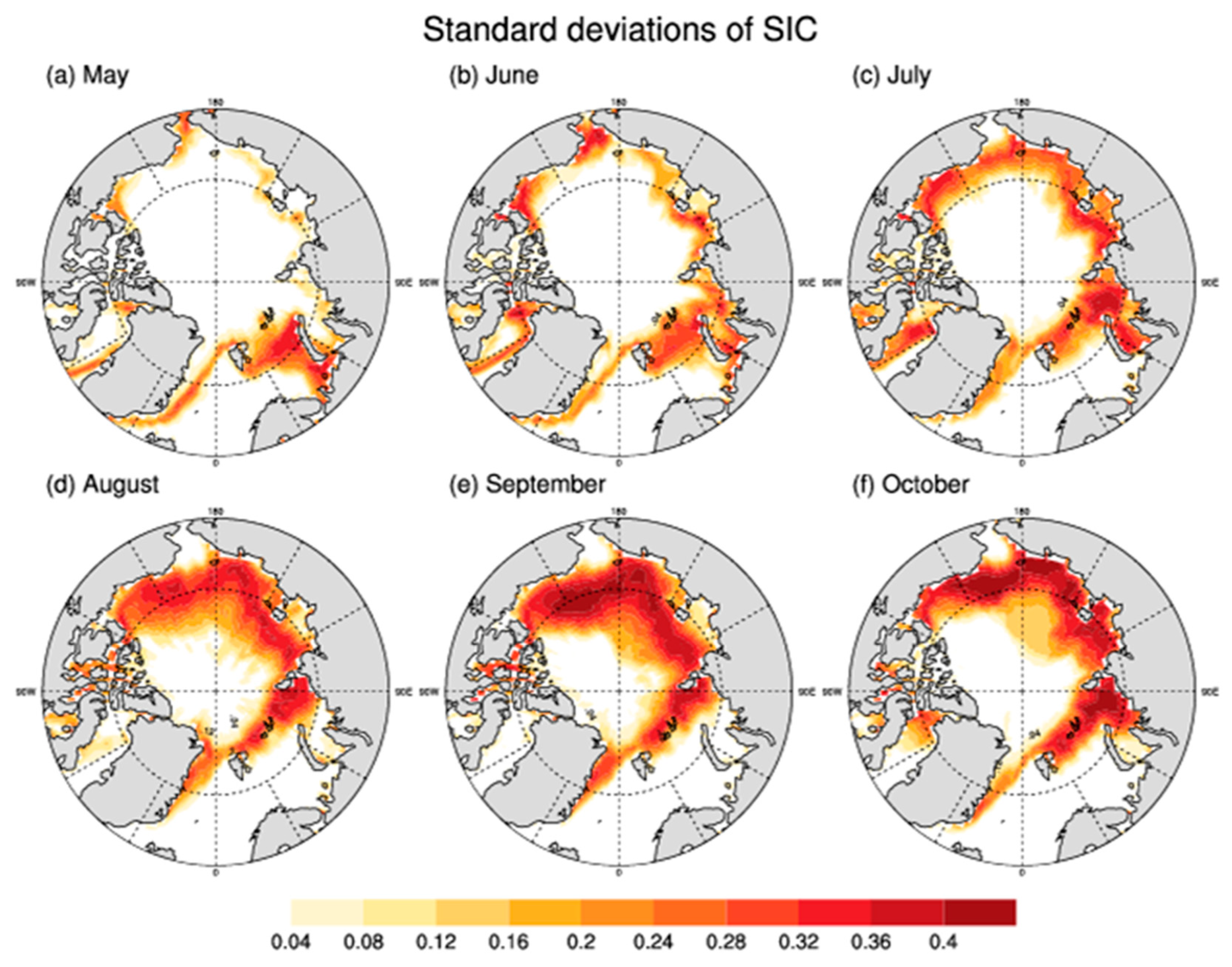
Figure 1 and Figure 2 show the spatial distribution of the SIC climatology and standard deviation from May to October for the period 1979 to 2017, respectively. As can be seen from Figure 1, the Arctic sea ice is in a continuously melting period from June to September and begins to condense in October. It shows that the low-latitude sea ice begins to melt first, and gradually forms an ice-free circle in the marginal sea. In September, the sea ice extent was the smallest. At this time, the Bering Sea, Kara Sea, Baffin Bay and the coastal areas of Chukchi Sea, East Siberian Sea, Laptev Sea and Barents Sea have almost no sea ice coverage. The high-latitude sea ice in the Beaufort Sea, Chukchi Sea, East Siberia Sea, Laptev Sea and Barents Sea are also significantly reduced during early summer, and the areas covered by perennial ice is gradually shrinking, as it retreats to the middle of the Arctic Ocean (within 75° N). In September, the sea ice in the whole coastal zone disappears and forms a wide open water body in the coastal sea area.
We describe the sea ice variability by calculating the standard deviation of the SIC. As shown in Figure 2, the spatial distribution of the SIC variability mainly shows a zonal distribution, and the high-value area mainly located near the ice boundary of the sea ice climatology. The summer sea ice anomaly centers basically appear in the Kara Sea, Laptev Sea, East Siberian Sea, Chukchi Sea and Beaufort Sea. In late summer, there is no ice on the North Pacific side, so there is no sea ice variability. On the North Atlantic side, a sea ice anomaly exists only in the vicinity of the Bay of Baffin, the Greenland Sea and other high-latitude areas. Looking at Figure 1 and Figure 2, we can see that the sea ice has been in a melting stage from June to September. Low-latitude marginal sea ice around the coastal areas of Bering Sea, Kara Sea, Baffin Bay and Barents Sea melted completely in June and July. In the later period, there was no sea ice cover in these areas, and the sea ice variability was zero; but, this “ice-free” state has a great impact on shipping and climate change. Therefore, in this paper we chose the average sea ice from June to September (the whole melting period of sea ice) for in-depth discussion.
We calculated the average SIC standard deviation from June to September for the period 1979–2017, and its spatial distribution is shown in Figure 3a. According to the distribution of the large variability centers in different sea areas, the regional average sea ice indices are calculated, and the correlation coefficients between them can be obtained in Figure 3b. Combining sea ice in regions where the correlation coefficients pass a significant t-test, several key areas of sea ice anomalies (maximum sea ice variability) were determined. Therefore, considering the key areas of sea ice anomalies and the route of the Arctic shipping route, this study investigates the spatial and temporal distribution of sea ice in the following key sea areas of the Arctic shipping route, including (1) the Barents Sea and the Kara Sea in the Northeast Channel; (2) the East Siberian Sea and the Laptev Sea in the Northeast Passage; and (3) the Beaufort Sea and the Canadian Arctic Archipelago in the Northwest Passage. These areas nearly cover the entire Arctic waterway. Studying the characteristics of sea ice changes in these sea areas in summer and making timely prediction of their anomalous changes can provide much-needed ice information for Arctic activities.
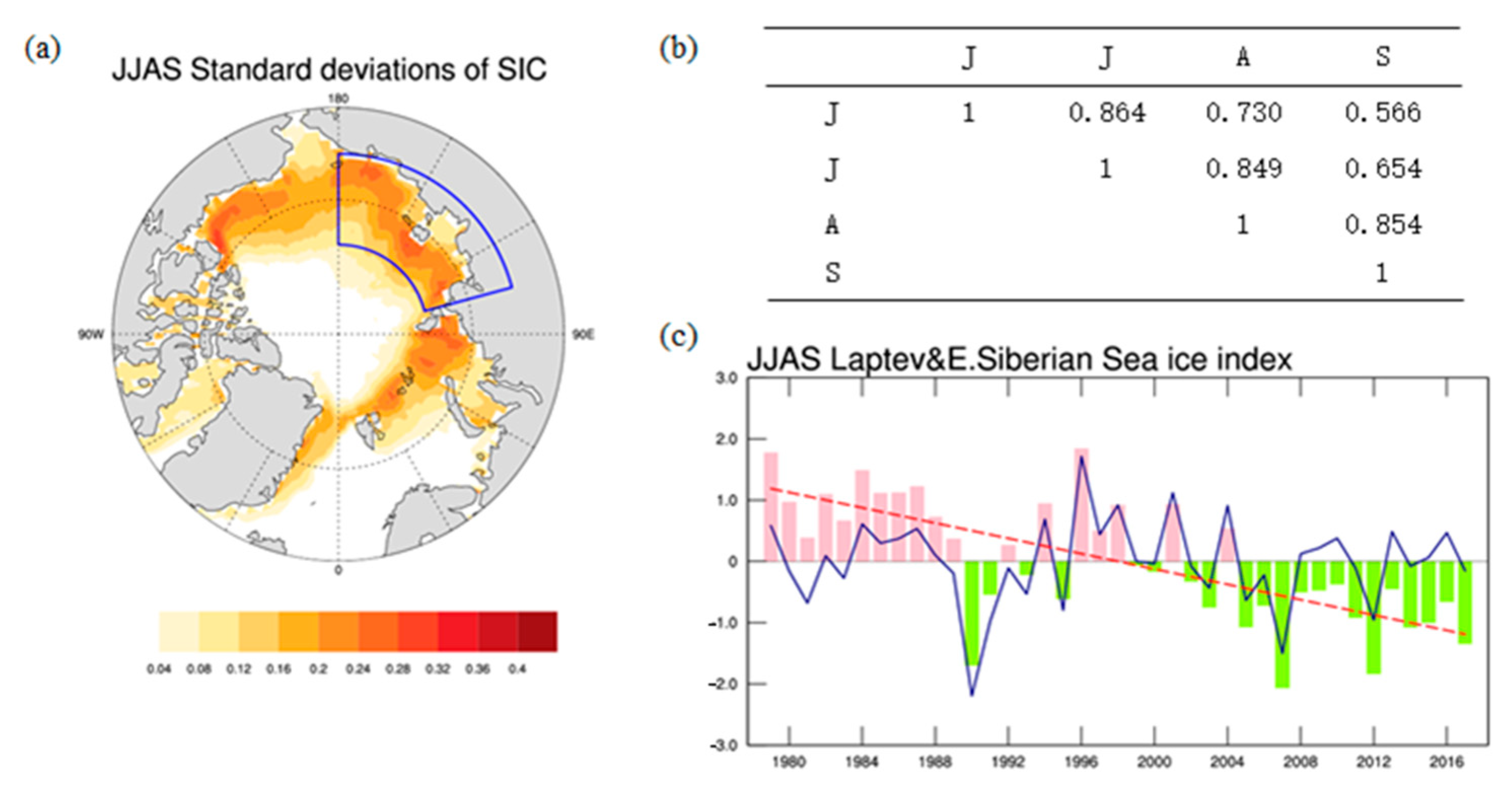
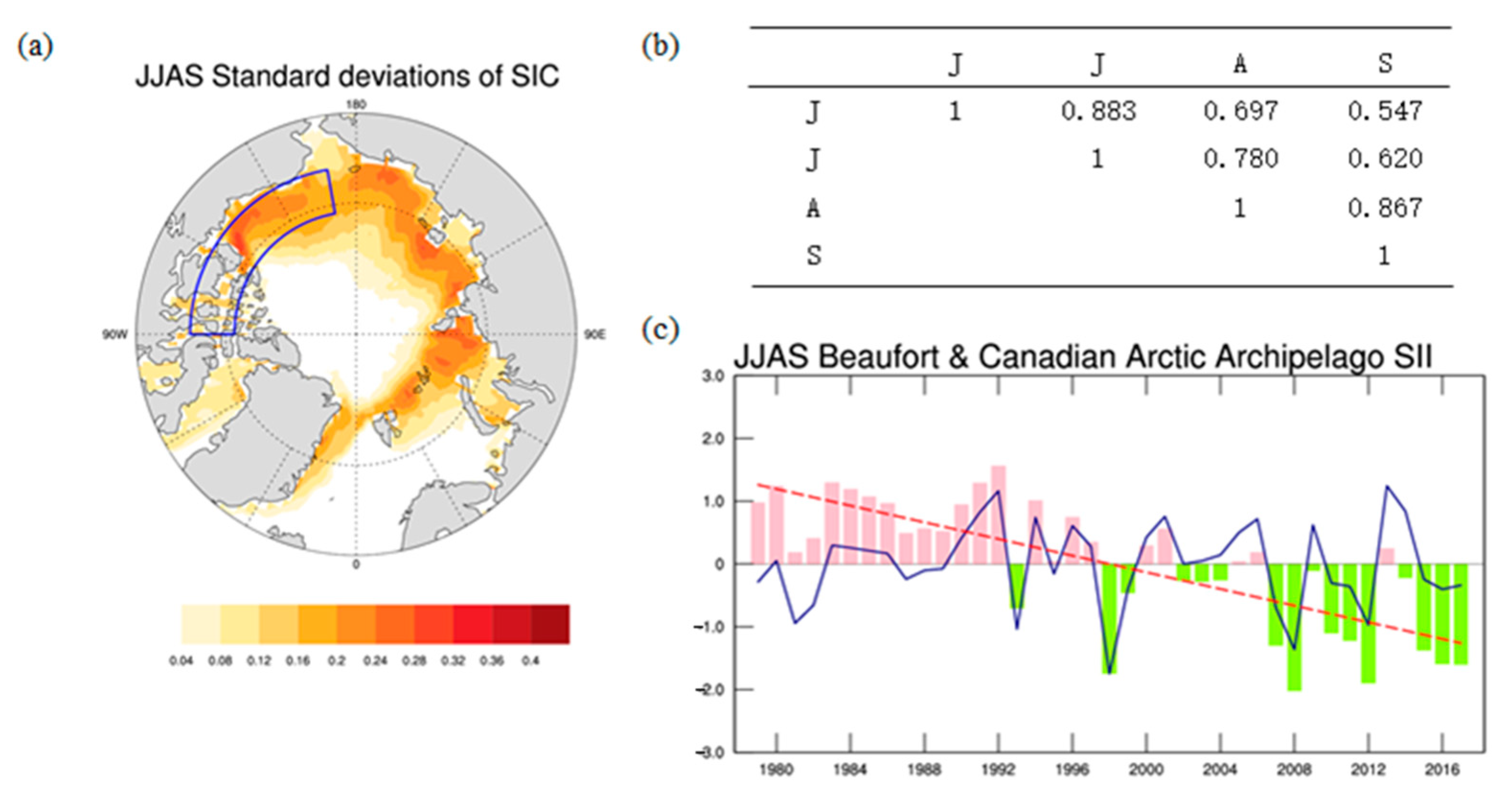
We defined the time series of the regional average SIC variability in the Barents Sea–Kara Sea (BK), East Siberian Sea–Laptev Sea (EL) and the Beaufort Sea–Canadian Arctic Archipelago (BC) area (in the blue frames of Figure 4, Figure 5 and Figure 6) from June to September 1979 to 2017 as the BK, EL and BC sea ice indices (pink-green bars in the Figure 4, Figure 5 and Figure 6), which is the number of standard deviations away from the average regional JJAS (the melt-season) sea ice concentration. Then we defined the detrended sea ice indices as the sea ice index (SII), since the focus here is on the interannual variations of the SIC rather than the long-term trend (blue carves in the Figure 4, Figure 5 and Figure 6). We calculated the correlation of these indices in June, July, August and September, and the correlation coefficients have all passed a certain significant Student’s t-test (Figure 4, Figure 5 and Figure 6). Specifically, sea ice is in a melting state in these four months. It is reasonable to study and discuss the average SIC of the four months.

4. The Leading Predictable Modes

Identifying the predictors is the first step in the model specification. As far as the rapid reduction of Arctic sea ice is concerned, its mechanism is mainly related to global warming. One of the most important global warming progresses is related to the rapid warming of the tropical and extra-tropical oceans. The predictability originates from the interactions between the atmosphere and ocean. Therefore, the abnormal changes in the SST and the related atmospheric circulation anomalies may be the key factors leading to the rapid melting of Arctic sea ice.
In this study, the seasonal leading role of the SST for the SIC is used to build statistical seasonal prediction models, and the PLSR method is used to find the spatial distribution of the SST anomalies before the SIC anomalies occur. First, the spring (March–April–May) SST anomaly field is used as predictors to establish a prediction equation, when the relationships between the predictors and the predictand are generally the greatest. Based on the measured SII, which is standardized according to its corresponding time period and the previous data of the SST field, the key area of SST that has the best correlation with sea ice anomaly is selected through multiple sensitivity tests to determine the sea area range of the prediction factor field Xij. Here, subscript j denotes the number of grid points in the selected critical area of SST after eliminating the missing data. Forecast Yi is the subsequent SII, which is a predictable one dimensional time series. The comprehensive variable Z can be understood as the main distribution pattern of SST, which is closely related to sea ice change revealed by the PLSR method; also, the SST field and sea ice have the best explanatory ability in the early stage.
The PLSR method is used to find the best SST mode with the best correlation between the SST in the early spring and the BK SII. As can be seen from Figure 7, the first two modes of PLSR have statistical significance. The first mode can explain 15.48% of the SST change and 53.84% of the sea ice change. The second mode can explain 20.79% of the SST change and 19.11% of the sea ice change. The first mode has an interdecadal variation similar to the AMO [57], and the corresponding time series shows interdecadal variation. The second mode is related to an AO-like or NAO-like SST pattern [58], and its time series shows interannual variation. This reflects the consideration of multi-scale interaction, which makes the prediction results more accurate. These two SST modes can provide a predictable source of sea ice in the BK Sea from June to September.
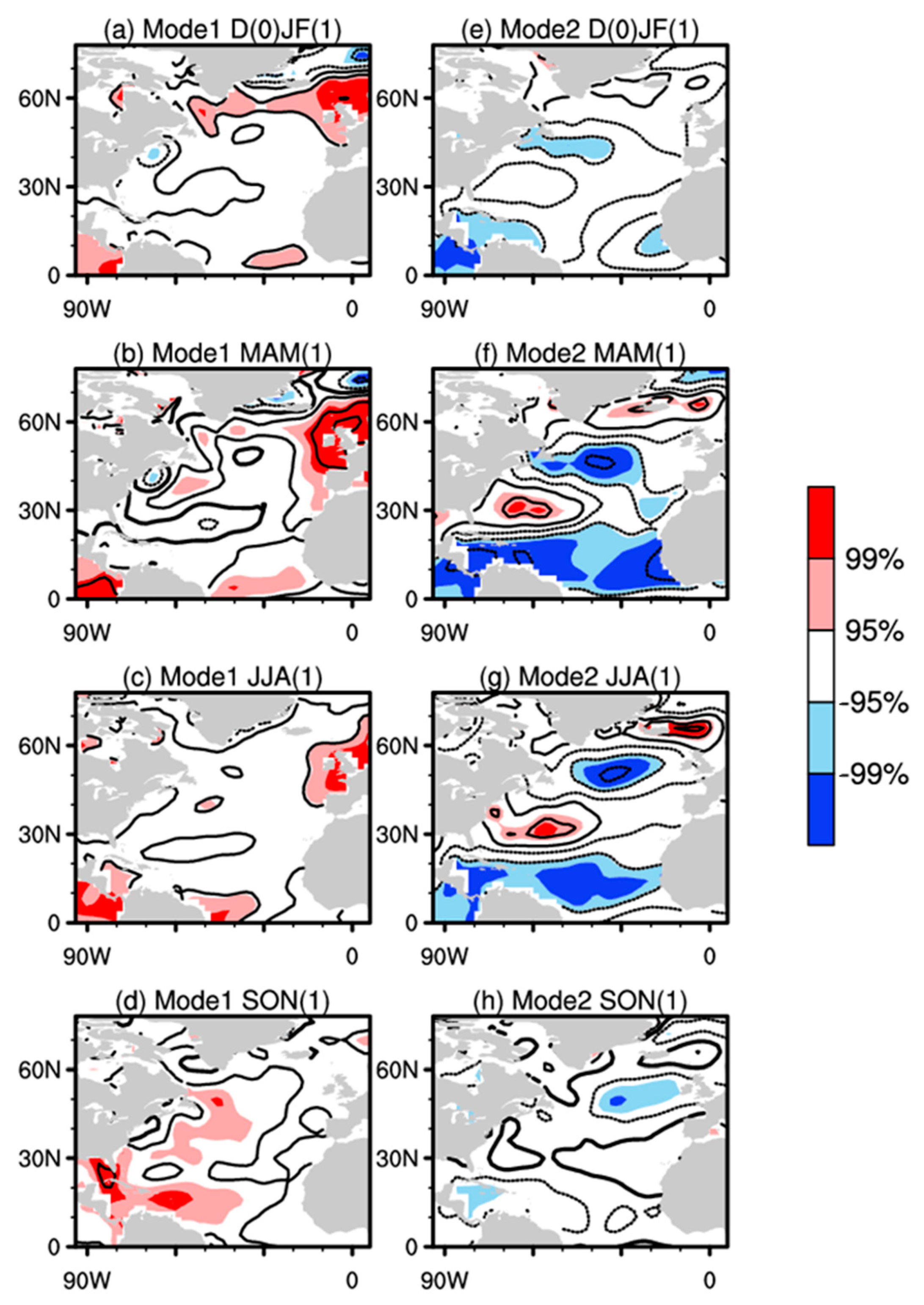
In order to reveal the physical significance of the above two PLSR SST modes, we analyzed the evolution characteristics of the SST field corresponding to the two PLSR SST modes. Figure 8 shows the development of the corresponding SST field from early winter to autumn. It can be seen that the second mode of PLSR has an obvious AO distribution pattern in the early spring, and this SST distribution pattern can last until the subsequent summer, which exerts a direct effect on summer sea ice change. It shows that the second mode has a certain degree of persistence, and this stability can provide strong support for prediction.
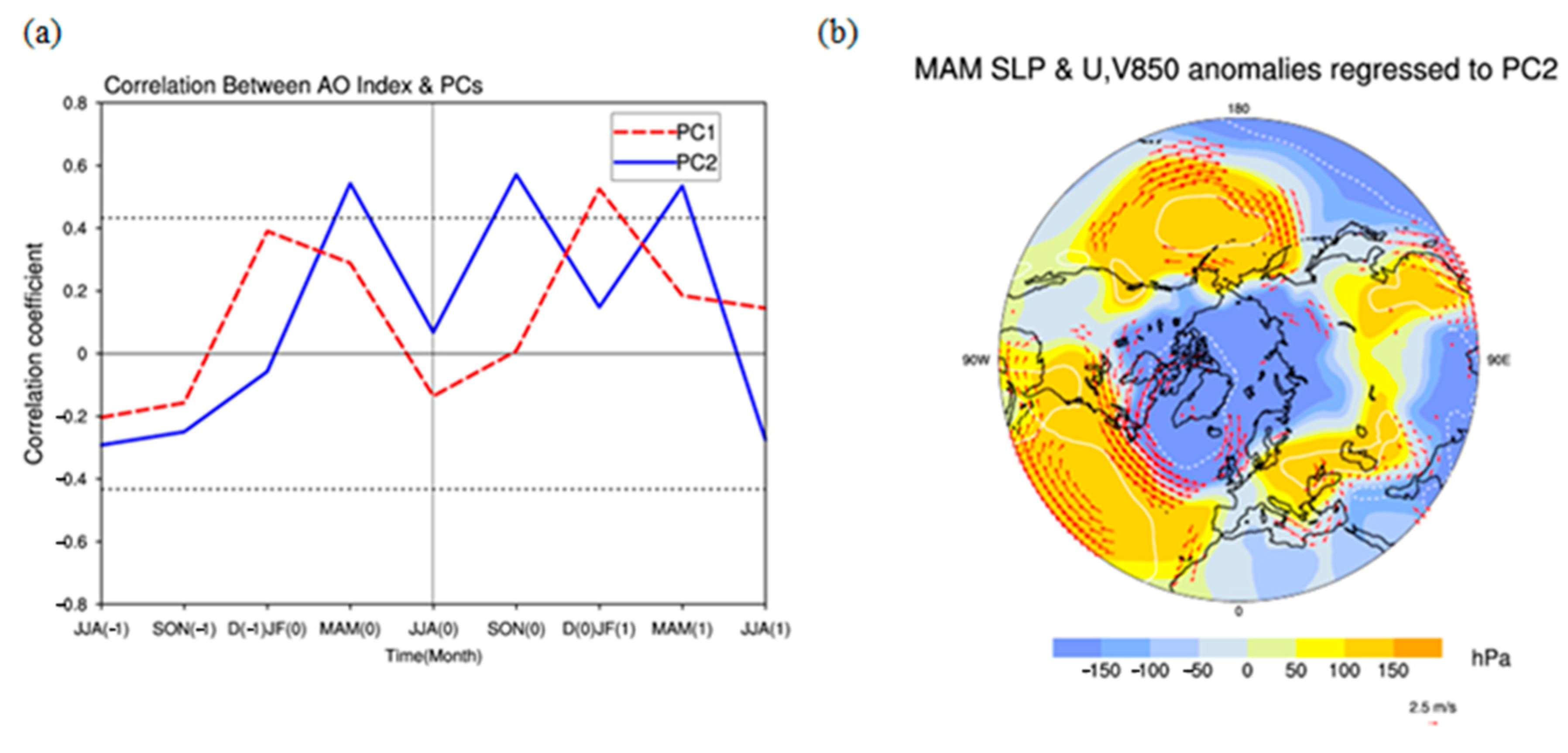
We also calculated the lead–lag correlation between the time series corresponding to the two modes and AO index (Figure 9a). The two modes are first presented in Figure 7, in which case the predictand is spring SSTs and summer SIC, which are constant. While, the AO index is being averaged for each season, which can be regard as variable. It can be found that the correlation between the second mode time series and AO index passed the 95% significance t-test in the early spring, which shows that the second mode is obviously related to the change in AO. We linearly regressed the time series with prior spring U and V winds at the 850 hPa levels and SLP; the responses of the atmospheric circulation suggest an obvious AO-positive phase (Figure 9b). Low-pressure anomalies occur in the polar region while high-pressure anomalies are located in the middle latitudes. It indicates that the sea ice changes in the BK Sea may be closely related to the changes in AO in the early spring, and the anomalous signals of AO may lead to the anomalous changes in sea ice in the BK Sea from June to September in summer.
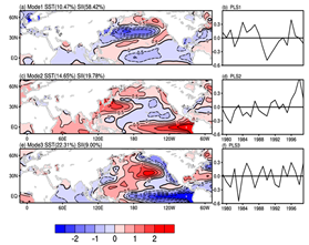
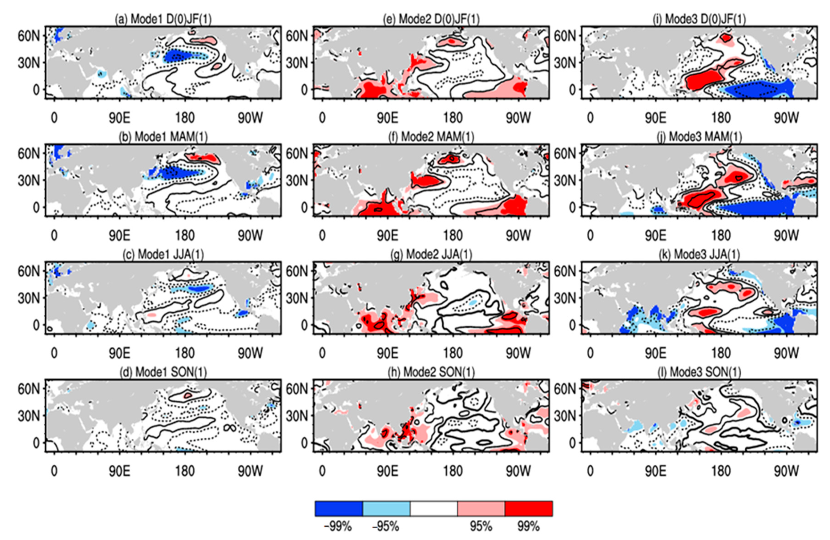
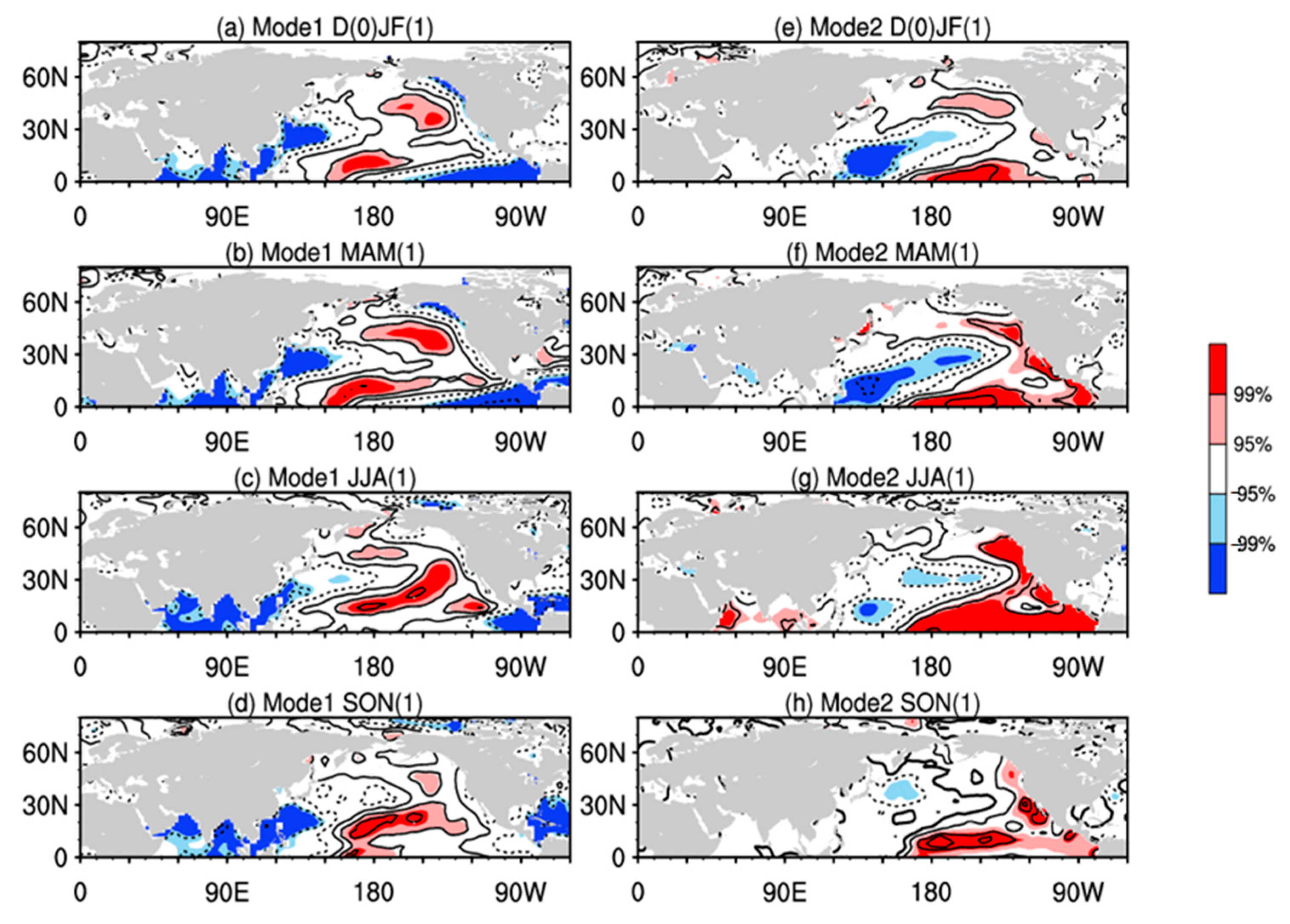
Similarly, we use the PLSR method to find the best SST modes for the EL and BC sea ice indices. The results are shown in Figure 10 and Figure 11. As can be seen from Figure 10, sea ice in the EL Sea is associated with the PDO-like SST modes [59]. Specifically, the Mode 1 matches a positive PDO signal for the northern Pacific only. Mode 2 matches a positive PDO signal for the tropical Pacific and Indian Ocean but not the northern Pacific—especially not east of Japan; that is a bit more El Niño-like. Mode 3 looks the most PDO-like overall (a negative PDO pattern/La Niña). The first three modes of PLSR have statistical significance, totally accounting for 47.43% of the SST changes and 87.2% of the SII changes. As for the BC SII, the first two SST modes have statistical significance, explaining the variance contribution of 43.08% SST change and 49.26% SSI change (Figure 11). As can be seen from the chart, sea ice in the BC area is associated with SST modes similar to PDO or ENSO. The first mode shows the cold SST in the tropical region and the equatorial Pacific region. In addition to the horseshoe-shaped SST distribution in the Northwest Pacific, the second mode also has significant, warm SST signals in the tropics, which is more consistent with PDO or ENSO—especially an El Niño pattern [60]. These SST modes can provide predictive sources for prediction. The corresponding evolution patterns of the SST modes are shown in Figure 12 and Figure 13.
These SST modes searched by the PLSR method indicate the precursory signals of the sea ice anomalies in early spring ahead of summer. They contain the information of the interannual to interdecadal oscillation signals (multi-scale interaction), such as AO, ENSO, PDO and AMO, which have a certain persistence. They can be used as the prediction factor field of the prediction model. Therefore, in the next study, we will use these SST modes to further establish the PE PLSR model to predict the SII.

5. PE PLSR Model Building

5.1. Modeling Process

In this study, the PE PLSR prediction model was established by reconstructing the SII, and independent prediction experiments were carried out. Modeling divides the whole data set into two parts. Firstly, using the data of the first 21 years (1979–1999) for regression training, this time is long enough to be used as the background field of reliable modeling and get the model of the training period. Then, the next 18 years (2000–2017) were taken as the actual forecast period, and the predicted value was compared with the true value to verify the prediction ability of the model.
The predictive equation we established is as follows (SII represents the time series of Arctic SII):
SII = SST × Beta + SIIresidual
SIIfit = SST × Beta, SII = SIIfit + SIIresidual
Here, SST represents the SST field and Beta is the regression coefficient matrix.
SIIresidual = SIIobserve − SIIfit
The specific process of model building and forecasting ability testing is as follows. During the model training and modeling period, the mean SST in spring 1979–1999 and the measured SII in 1979–1999 were used to fit the model in accordance with the PLSR modeling steps. Then, a stable regression equation of SII with respect to the SST field was established. The SII time series simulated during the training period of the corresponding model was obtained by introducing the data of the annual SST field.
In the actual forecast period of the model, it is assumed that we will forecast the SII in 2000. Firstly, the regression coefficient matrix Beta: SIIfit (1979–1999) = SST (1979–1999) × Beta and SIIresidual (1999) = SIIobserve (1999) − SIIfit (1999) were calculated according to the above prediction equation. Then, the new observed data of the 1996 SST field were input and SIIfit (2000) = SST (1999) × Beta, SII (2000) = SIIfit (2000) + SIIresidual (1999) were obtained.
In the process of modeling, through many sensitivity tests, we find that the new Beta and residuals can be obtained by inputting the new SST data and actual flux index into the equation every year, and then putting the new residuals into the model operation can improve the prediction skills of the model. Because of the uncertainty of the model system, the weakening factor is introduced to smooth the system error.

5.2. Model Prediction Effect and Performance Evaluation

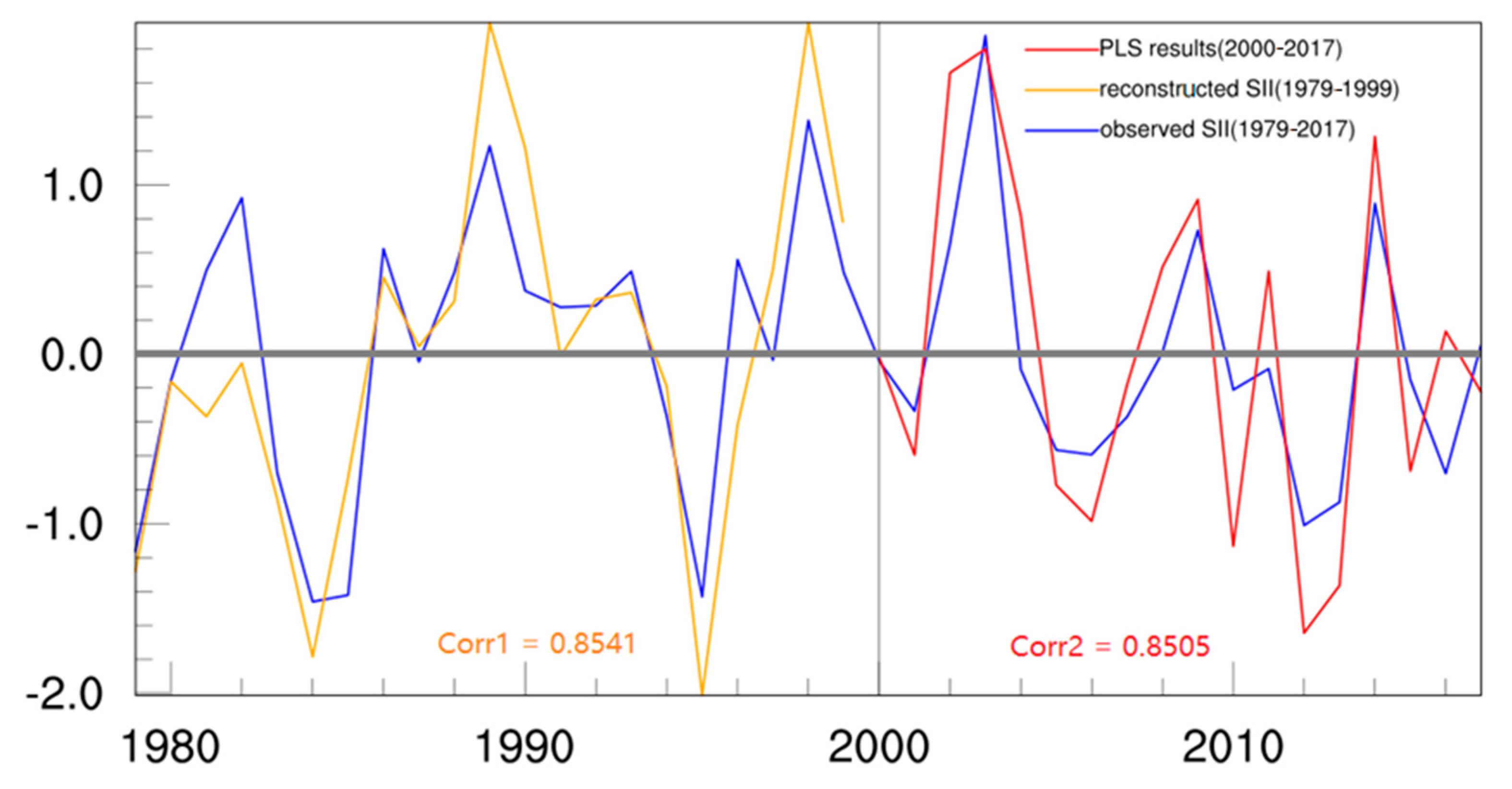
By calculating the correlation coefficient between the actual SII series and the simulation results, we can judge the fitting ability of the model, and calculate the correlation between the measured SII and the prediction results to obtain the actual prediction skills of the model. As shown in Figure 4, the blue solid line represents the actual SII, the yellow solid line is the SII simulated by the model training in 1979–1999, and the red solid line is the SII actually predicted by the model in 2000–2017. Corr1 is the correlation coefficient between the PE PLSR simulation and the actual SII in 1979–1999, and Corr2 is the correlation coefficient between the PE PLSR prediction and the actual SII in 2000–2017. Based on the first two SST modes, we construct the PE PLSR model to predict the BK SII. As shown in Figure 14, the correlation between the simulation period and the forecast period reaches 0.8541 and 0.8505, and the correlation coefficients pass the significance t-test with a confidence level of 99%, which shows that the established model has a high prediction level in both the simulation and prediction periods.
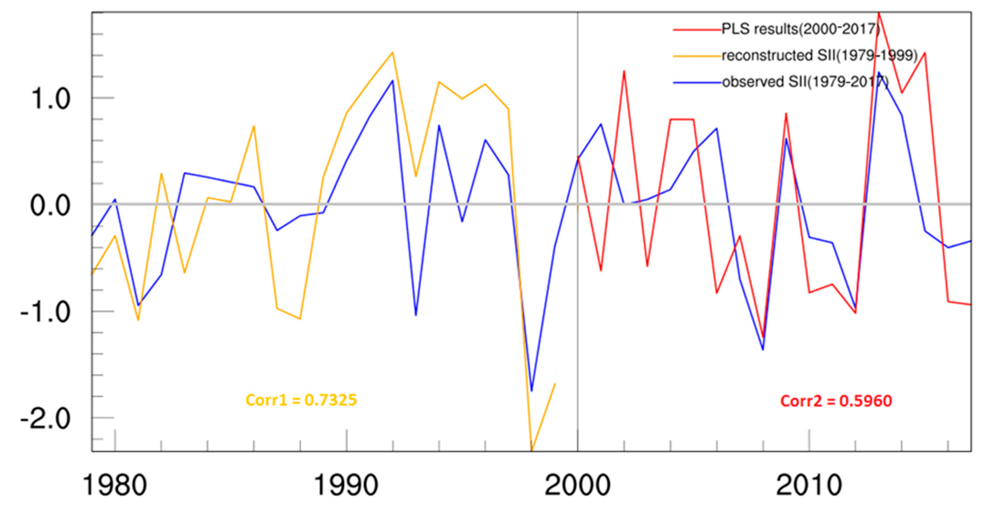
Similarly, based on the first three SST modes, we construct the PE PLSR model to predict the SII of the EL Sea. As shown in Figure 15, the correlation between the measured SII and the model simulated index is 0.9331, and the correlation between the predicted index and the predicted index is 0.6321. All of them are statistically significant at or above the 99% confidence level. The prediciton skills are relatively high. What is more, we constructed the PE PLSR model to forecast the SII in the BC area using the first two SST modes. The correlation coefficient between the simulated SII and measured SII is 0.7325 and 0.5960 (Figure 16), which all passed the 99% significance t-test. The model has a good predictive performance for sea ice anomalies in the area of the BC during the target months.

6. Discussion and Conclusions

The summer Arctic SIC has decreased dramatically during the past decade, which may bring about unpredictable climate impact and may accelerate the maritime transport in the Arctic shipping route as well. Accurate prediction of the Arctic summer sea ice draws great interests but remains an ongoing challenge for scientists.
In this study, we carried out the seasonal prediction of summer SIC by statistical approaches using the PLSR model to predict the sea ice variation in three major parts of the Arctic shipping route. This approach combines statistical analysis with physical thinking. Wang et al. [61] showed there is good agreement between the sea ice dataset used here and the more widely used NSIDC record for the satellite period. The data we used are relatively reliable. Although the resolution of the data is not relatively high, the difference may be negligible if we use seasonal average sea ice data over a large spatial range. The previous SST in spring was chosen as predictors to establish the statistical models, and the models were established by the SST modes from the PLSR method. The high absolute values of the correlation coefficient suggest that these models have a fabulous ability in reproducing the sea ice change, and we confirmed that the models provided moderate seasonal prediction results in the lead time of one season. Therefore, the model is recommended for the prediction of Arctic summer SIC.
Although this model can present good simulation results in all three regions, the Barents–Kara region has a stronger relationship in the 2000–2017 period than the Laptev–East Siberian or Beaufort–Canadian Archipelago regions. In other words, the Atlantic side has more predictability than the Pacific side with this method. It is apparent that, while the ice cover in the Arctic is retreating rapidly, the character of the changing ice is very different in the Atlantic and Pacific sectors [62,63,64,65]. A number of studies showed that the Barents Sea is one of the Arctic regions with the largest sea ice variability at different time scales [66,67,68] and the air–sea temperature differences in the Barents Sea are extremely large [69,70]. We can expect that sea ice change in the Barents Sea will greatly affect the heat release, thus affecting the local and possibly large-scale climatic conditions. This will provide a potential for climate prediction [71].
The Arctic will be a window for future climate change, and the Arctic region is very sensitive to climate change. If the Arctic continues to warm, we will encounter extreme weather more frequently [72,73]. Arctic climate change has profound impacts on the cryosphere, notably via shrinking the sea-ice cover [74]. It is crucial to make reasonable predictions of Arctic summer sea ice, and the results from this paper can help provide more timely and effective forecasting services for Arctic scientific research and marine activities.

Author Contributions

Conceptualization, X.Y. and Z.W.; methodology, X.Y. and Z.W.; software, X.Y.; validation, X.Y. and Z.W.; formal analysis, X.Y. and Z.W.; investigation, X.Y. and Z.W.; resources, X.Y. and Z.W.; data curation, X.Y. and Z.W.; writing—original draft preparation, X.Y. and Z.W.; writing—review and editing, Z.W.; visualization, Z.W.; supervision, X.Y. and Z.W.; project administration, Z.W.; funding acquisition, Z.W. All authors have read and agreed to the published version of the manuscript.

Funding

This work is jointly supported by the Second Tibetan Plateau Scientific Expedition and Research (STEP) program (Grant No. 2019QZKK0102), National Natural Science Foundation of China (Grant Nos. 91937302 and 41790475) and the National Key R&D Program of China (Grant Nos. 2019YFC1509100 and2016YFA0601801).

Institutional Review Board Statement

Our study did not involve humans.

Informed Consent Statement

Our study did not involve humans.

Data Availability Statement

Our data are publicly available, and the specific website can refer to references.

Conflicts of Interest

The authors declare no conflict of interest.

References

  1. Serreze, M.; Barry, R. Processes and impacts of Arctic amplification: A research synthesis. Glob. Planet. Chang. 2011, 77, 85–96. [Google Scholar] [CrossRef]
  2. Francis, J.; Vavrus, S. Evidence linking arctic amplification to extreme weather in mid-latitudes. Geophys. Res. Lett. 2012, 39, L06801. [Google Scholar] [CrossRef]
  3. Grunseich, G.; Wang, B. Arctic sea ice patterns driven by the Asian summer monsoon. J. Clim. 2016, 29, 9097–9112. [Google Scholar] [CrossRef]
  4. Kerr, R. Will the Arctic Ocean lose all its ice? Science 1999, 286, 1828. [Google Scholar] [CrossRef]
  5. Stroeve, J.; Serreze, M.; Fetterer, F.; Arbetter, T.; Meier, W.; Maslanik, J.; Knowles, K. Tracking the Arctic’s shrinking ice cover: Another extreme September minimum in 2004. AGU Fall Meet. Abstr. 2005, 32, L04501. [Google Scholar] [CrossRef] [Green Version]
  6. Serreze, M.; Holland, M.; Stroeve, J. Perspectives on the Arctic’s shrinking sea-ice cover. Science 2007, 315, 1533–1536. [Google Scholar] [CrossRef] [Green Version]
  7. Stein, R.; Fahl, K.; Gierz, P.; Niessen, F.; Lohmann, G. Arctic Ocean sea ice cover during the penultimate glacial and the last interglacial. Nat. Commun. 2017, 8, 373. [Google Scholar] [CrossRef]
  8. Yu, L.; Zhong, S.; Zhou, M.; Lenschow, D.H.; Sun, B. Revisiting the Linkages between the Variability of Atmospheric Circulations and Arctic Melt-Season Sea Ice Cover at Multiple Time Scales. J. Clim. 2019, 32, 1461–1482. [Google Scholar] [CrossRef]
  9. Ogi, M.; Wallace, J.M. Summer minimum Arctic sea ice extent and the associated summer atmospheric circulation. Geophys. Res. Lett. 2007, 34, L12705. [Google Scholar] [CrossRef] [Green Version]
  10. Yamamoto, K.; Tachibana, Y.; Honda, M.; Ukita, J. Intra-seasonal relationship between the Northern Hemisphere sea ice variability and the North Atlantic Oscillation. Geophys. Res. Lett. 2006, 33, L14711. [Google Scholar] [CrossRef] [Green Version]
  11. Wang, J.; Wu, B.; Tang, C.; Walsh, J.; Ikeda, M. Seesaw structure of subsurface temperature anomalies between the Barents Sea and the Labrador Sea. Geophys. Res. Lett. 2004, 31, L19301. [Google Scholar] [CrossRef]
  12. Thompson, D.W.; Wallace, J.M. The Arctic Oscillation signature in the wintertime geopotential height and temperature fields. Geophys. Res. Lett. 1998, 25, 1297–1300. [Google Scholar] [CrossRef] [Green Version]
  13. Deser, C.; Walsh, J.E.; Timlin, M.S. Arctic sea ice variability in the context of recent atmospheric circulation trends. J. Clim. 2000, 13, 617–633. [Google Scholar] [CrossRef]
  14. Hu, A.; Rooth, C.; Bleck, R.; Deser, C. NAO influence on sea ice extent in the Eurasian coastal region. Geophys. Res. Lett. 2002, 29, 2053. [Google Scholar] [CrossRef] [Green Version]
  15. Rigor, I.; Wallace, J.M.; Colony, R.L. Response of sea ice to the Arctic Oscillation. J. Clim. 2002, 15, 2648–2663. [Google Scholar] [CrossRef] [Green Version]
  16. Ding, Q.; Wallace, J.M.; Battisti, D.S.; Steig, E.J.; Gallant, A.J.E.; Kim, H.-J.; Geng, L. Tropical forcing of the recent rapid Arctic warming in northeastern Canada and Greenland. Nature 2014, 509, 209–212. [Google Scholar] [CrossRef] [PubMed]
  17. Ding, Q.; Schweiger, A.; L’Heureux, M.; Battisti, D.S.; Po-Chedley, S.; Johnson, N.C.; Blanchard-Wrigglesworth, E.; Harnos, K.; Zhang, Q.; Eastman, R.; et al. Influence of high-latitude atmospheric circulation changes on summertime Arctic sea ice. Nat. Publ. Group 2017, 7, 289–295. [Google Scholar] [CrossRef]
  18. Yu, L.; Wu, Z.; Zhang, R.; Yang, X. Partial least regression approach to forecast the East Asian winter monsoon using Eurasian snow cover and sea surface temperature. Clim. Dyn. 2018, 51, 4573–4584. [Google Scholar] [CrossRef]
  19. Ferguson, S.H.; Taylor, M.K.; Messier, F. Influence of sea ice dynamics on habitat selection by polar bears. Ecology 2000, 81, 761–772. [Google Scholar] [CrossRef]
  20. Overland, J.; Wood, K.; Wang, M. Large-scale atmospheric circulation changes are associated with the recent loss of Arctic sea ice Tellus A. Dyn. Meteorol. Oceanogr. 2010, 62, 1–9. [Google Scholar] [CrossRef] [Green Version]
  21. Overland, J.; Wood, K.; Wang, M. Warm Arctic–cold continents: Climate impacts of the newly open Arctic Sea. Polar Res. 2011, 30, 15787. [Google Scholar] [CrossRef]
  22. Ivanov, V.; Varentsov, M.; Matveeva, T.; Repina, I.; Artamonov, A.; Khavina, E. Arctic sea ice decline in the 2010s: The increasing role of the ocean-air heat exchange in the late summer. Atmosphere 2019, 10, 184. [Google Scholar] [CrossRef] [Green Version]
  23. Kumar, A.; Perlwitz, J.; Eischeid, J.; Quan, X.; Xu, T.; Zhang, T.; Hoerling, M.; Jha, B.; Wang, W. Contribution of sea ice loss to arctic amplification. Geophys. Res. Lett. 2010, 37. [Google Scholar] [CrossRef] [Green Version]
  24. Guemas, V.; Blanchard, E.; Chevallier, M.; Day, J.; Déqué, M.; Doblas, F.; Fuckar Neven, S.; Geme, A.; Hawkins, E.; Keeley, S.; et al. A review on Arctic sea-ice predictability and prediction on seasonal to decadal time-scales. Q. J. R. Meteorol. Soc. 2016, 142, 546–561. [Google Scholar] [CrossRef]
  25. Petty, A.A.; Schröder, D.; Stroeve, J.C.; Markus, T.; Miller, J.; Kurtz, N.T.; Feltham, D.L.; Flocco, D. Skillful spring forecasts of September Arctic sea ice extent using passive microwave sea ice observations. Earths Future 2017, 5, 254–263. [Google Scholar] [CrossRef]
  26. Wayand, N.E.; Bitz, C.M.; Blanchard, W. A Year—Round Subseasonal-to-Seasonal Sea Ice Prediction Portal. Geophys. Res. Lett. 2019, 46, 3298–3307. [Google Scholar] [CrossRef]
  27. Cruz-García, R.; Guemas, V.; Chevallier, M.; Massonnet, F. An assessment of regional sea ice predictability in the arctic ocean. Clim. Dyn. 2019, 53, 427–440. [Google Scholar] [CrossRef]
  28. Bushuk, M.; Msadek, R.; Winton, M.; Vecchi, G.A.; Gudgel, R.; Rosati, A. Skillful regional prediction of arctic sea ice on seasonal timescales. Geophys. Res. Lett. 2017, 44, 4953–4964. [Google Scholar] [CrossRef]
  29. Massonnet, F.; Fichefet, T.; Goosse, H. Prospects for improved seasonal arctic sea ice predictions from multivariate data assimilation. Ocean Model. 2015, 88, 16–25. [Google Scholar] [CrossRef]
  30. Melia, N.; Haines, K.; Hawkins, E.; Day, J.J. Towards seasonal Arctic shipping route predictions. Environ. Res. Lett. 2017, 12, 084005. [Google Scholar] [CrossRef]
  31. Yang, C.; Liu, J.; Xu, S. Seasonal arctic sea ice prediction using a newly developed fully coupled regional model with the assimilation of satellite sea ice observations. J. Adv. Modeling Earth Syst. 2020, 12, e2019MS001938. [Google Scholar] [CrossRef] [Green Version]
  32. Silva, D.; Arampath, L.; Yamaguchi, H.; Ono, J. Ice-ocean coupled computations for sea-ice prediction to support ice navigation in arctic sea routes. Polar Res. 2015, 34, 25008. [Google Scholar] [CrossRef] [Green Version]
  33. Zhang, J.; Steele, M.; Lindsay, R.; Schweiger, A.; Morison, J. Ensemble 1-year predictions of arctic sea ice for the spring and summer of 2008. Geophys. Res. Lett. 2008, 35, L08502. [Google Scholar] [CrossRef] [Green Version]
  34. Kattsov, V.; Ryabinin, V.; Overland, J.; Serreze, M.; Visbeck, M.; Walsh, J.; Meier, W.; Zhang, X. Arctic sea ice change: A grand challenge of climate science. J. Glaciol. 2010, 56, 1115–1121. [Google Scholar] [CrossRef] [Green Version]
  35. Stroeve, J.; Hamilton, L.; Bitz, C.; Blanchard, E. Predicting September sea ice: Ensemble skill of the search sea ice outlook 2008–2013. Geophys. Res. Lett. 2014, 41, 2411–2418. [Google Scholar] [CrossRef] [Green Version]
  36. Vihma, T. Effects of arctic sea ice decline on weather and climate: A review. Surv. Geophys. 2014, 35, 1175–1214. [Google Scholar] [CrossRef] [Green Version]
  37. Kim, Y.; Kim, H.; Choi, Y.; Kim, W.; Kim, H. Development of statistical seasonal prediction models of arctic sea ice concentration using CERES absorbed solar radiation. J. Atmos. Sci. 2016, 52, 467–477. [Google Scholar] [CrossRef]
  38. Hawkins, E.; Tietsche, S.; Day, J.; Melia, N.; Haines, K.; Keeley, S. Aspects of designing and evaluating seasonal-to-interannual Arctic sea-ice prediction systems. Q. J. R. Meteorol. Soc. 2016, 142, 672–683. [Google Scholar] [CrossRef] [Green Version]
  39. Wu, Z.; Wang, B.; Li, J.; Jin, F. An empirical seasonal prediction model of the East Asian summer monsoon using ENSO and NAO. J. Geophys. Res. Atmos. 2009, 27, 114. [Google Scholar] [CrossRef]
  40. Wu, Z.; Li, J.; Jiang, Z.; He, J. Predictable climate dynamics of abnormal East Asian winter monsoon: Once-in-a-century snowstorms in 2007/2008 winter. Clim. Dyn. 2011, 37, 1661. [Google Scholar] [CrossRef]
  41. Wold, S.; Ruhe, A.; Wold, H.; Dunn, I. The collinearity problem in linear regression. The partial least squares (PLS) approach to generalized inverses. J. Sci. Stat. Comput. 1984, 5, 735–743. [Google Scholar] [CrossRef] [Green Version]
  42. Yeniay, Q.; Goktas, A. A comparison of partial least square regression with other prediction methods. Acettepe J. Math. Stat. 2002, 31, 99–101. [Google Scholar]
  43. Haenlein, M.; Kaplan, A. A beginner’s guide to partial least squares analysis. Underst. Stat. 2004, 3, 283–297. [Google Scholar] [CrossRef]
  44. Tan, Y.; Shi, L.; Tong, W.; Huang, G.; Wang, C. Multi-class tumor classification by discriminant partial least squares using microarray gene expression data and assessment of classification models. Comput. Biol. Chem. 2004, 28, 235–243. [Google Scholar] [CrossRef] [PubMed]
  45. Haaland, D.; Thomas, E. Partial least-squares methods for spectral analyses. 2. Application to simulated and glass spectral data. Anal. Chem. 1998, 60, 1202–1208. [Google Scholar] [CrossRef]
  46. Wold, S.; Sjöström, M.; Eriksson, L. PLS-regression: A basic tool of chemometrics. Chemom. Intell. Lab. Syst. 2011, 58, 109–130. [Google Scholar] [CrossRef]
  47. Udelhoven, T.; Emmerling, C.; Jarmer, T. Quantitative analysis of soil chemical properties with diffuse reflectance spectrometry and partial least-square regression: A feasibility study. Plant Soil 2003, 251, 319–329. [Google Scholar] [CrossRef]
  48. McIntosh, A.; Lobaugh, N. Partial least squares analysis of neuroimaging data: Applications and advances. Neuroimage 2004, 23, 250–263. [Google Scholar] [CrossRef]
  49. Zhang, H.; Qin, J.; Li, Y. Climatic background of cold and wet winter in southern China: Part I observational analysis. Clim. Dyn. 2011, 37, 2335–2354. [Google Scholar] [CrossRef]
  50. Wu, Z.; Lin, H.; Li, Y.; Tang, Y. Seasonal prediction of killing-frost frequency in South-Central Canada during the cool/overwintering-crop growing season. J. Appl. Meteorol. Climatol. 2013, 52, 102–113. [Google Scholar] [CrossRef]
  51. Wu, Z.; Yu, L. Seasonal prediction of the East Asian summer monsoon with a partial-least square model. Clim. Dyn. 2015, 46, 3067–3078. [Google Scholar] [CrossRef]
  52. Ye, X.; Wu, Z.; Wang, Z.; Shen, H.; Xu, J. Seasonal prediction of the Yangtze River runoff using a partial least squares regression model. Atmos. Ocean 2018, 56, 117–128. [Google Scholar] [CrossRef]
  53. Rayner, N.; Parker, D.; Horton, E.; Folland, C.; Alexander, L.; Rowell, D.; Kent, E.; Kaplan, A. Global analyses of sea surface temperature, sea ice, and night marine air temperature since the late nineteenth century. J. Geophys. Res. 2003, 108, 4407. [Google Scholar] [CrossRef]
  54. Smith, T.; Reynolds, R.; Peterson, T.; Lawrimore, J. Improvements to NOAA’s historical merged land-ocean surface temperature analysis (1880–2006). J. Clim. 2008, 21, 2283–2296. [Google Scholar] [CrossRef]
  55. Kalnay, E.; Kanamitsu, M.; Kistler, R.; Collins, W.; Deaven, D.; Gandin, L.; Zhu, Y. The NCEP/NCAR 40-year reanalysis project. Bull. Am. Meteorol. Soc. 1996, 77, 437–471. [Google Scholar] [CrossRef] [Green Version]
  56. Song, L.; Duan, W.; Li, Y.; Mao, J. A timescale decomposed threshold regression downscaling approach to forecasting South China early summer rainfall. Adv. Atmos. Sci. 2016, 33, 1071–1084. [Google Scholar] [CrossRef]
  57. Knight, J.; Folland, C.; Scaife, A. Climate impacts of the Atlantic Multidecadal Oscillation. Geophys. Res. Lett. 2006, 33, L17706. [Google Scholar] [CrossRef] [Green Version]
  58. Koenigk, T.; Mikolajewicz, U.; Jungclaus, J.H.; Kroll, A. Sea ice in the Barents Sea: Seasonal to interannual variability and climate feedbacks in a global coupled model. Clim. Dyn. 2008, 32, 1119–1138. [Google Scholar] [CrossRef] [Green Version]
  59. Newman, M.; Alexander, M.A.; Ault, T.R.; Cobb, K.M.; Deser, C.; Di Lorenzo, E.; Mantua, N.J.; Miller, A.J.; Minobe, S.; Nakamura, H.; et al. The Pacific Decadal Oscillation, Revisited. J. Clim. 2016, 29, 4399–4427. [Google Scholar] [CrossRef] [Green Version]
  60. Deser, C.; Alexander, M.A.; Xie, S.P.; Phillips, A.S. Sea surface temperature variability: Patterns and mechanisms. Annu. Rev. Mar. Sci. 2010, 2, 115. [Google Scholar] [CrossRef] [Green Version]
  61. Rui-Bo, W.A.; Shuanglin, L.I.; Zhe, H.A. Evaluation of the HadISST1 and NSIDC 1850 onward sea ice datasets with a focus on the Barents-Kara seas. Atmos. Ocean. Sci. Lett. 2018. [Google Scholar] [CrossRef] [Green Version]
  62. Serreze, M.C.; Crawford, A.D.; Stroeve, J.C.; Barrett, A.P.; Woodgate, R.A. Variability, trends, and predictability of seasonal sea ice retreat and advance in the Chukchi Sea. J. Geophys. Res. Ocean. 2016, 127. [Google Scholar] [CrossRef]
  63. Serreze, M.C.; Barrett, A.P.; Crawford, A.D.; Woodgate, R.A. Monthly variability in Bering Strait oceanic volume and heat transports, links to atmospheric circulation and ocean temperature, and implications for sea ice conditions. J. Geophys. Res. Ocean. 2019, 124, 9317–9337. [Google Scholar] [CrossRef]
  64. Wendler, G.; Shulski, M.; Moore, B. Changes in the climate of the Alaskan North Slope and the ice concentration of the adjacent Beaufort Sea. Theor. Appl. Climatol. 2009, 99, 67–74. [Google Scholar] [CrossRef]
  65. Woodgate, R.A.; Weingartner, T.; Lindsay, R. The 2007 Bering Strait oceanic heat flux and anomalous Arctic sea-ice retreat. Geophys. Res. Lett. 2010, 37. [Google Scholar] [CrossRef] [Green Version]
  66. Parkinson, C.; Cavalieri, D. Arctic sea ice variability and trends, 1979–2006. J. Geophys. Res. 2008, 113, C07003. [Google Scholar] [CrossRef]
  67. Screen, J.A.; Simmonds, I. Increasing fall-winter energy loss from the Arctic Ocean and its role in Arctic temperature amplification. Geophys. Res. Lett. 2010, 37, L16707. [Google Scholar] [CrossRef] [Green Version]
  68. Mikhailova, N.V.; Yurovsky, A.V. Analysis of Principal Components of the Sea Ice Concentration Fields in the Barents Sea. Phys. Oceanogr. 2017, 11–18. [Google Scholar] [CrossRef]
  69. Simonsen, K.; Haugan, P. Heat budgets of the Arctic Mediterranean and sea surface heat flux parameterizations for the Nordic Seas. J. Geophys. Res. 1996, 101, 6553–6576. [Google Scholar] [CrossRef]
  70. Årthun, M.; Eldevik, T.; Smedsrud, L.H.; Skagseth, Ø.; Ingvaldsen, R.B. Quantifying the Influence of Atlantic Heat on Barents Sea Ice Variability and Retreat. J. Clim. 2012, 25, 4736–4743. [Google Scholar] [CrossRef] [Green Version]
  71. Onarheim, I.H.; Eldevik, T.; Årthun Marius Ingvaldsen, R.B.; Smedsrud, L.H. Skillful prediction of barents sea ice cover. Geophys. Res. Lett. 2015, 42, 5364–5371. [Google Scholar] [CrossRef] [Green Version]
  72. Lee, M.Y.; Hong, C.C.; Hsu, H.H. Compounding effects of warm sea surface temperature and reduced sea ice on the extreme circulation over the extratropical north pacific and north America during the 2013–2014 boreal winter. Geophys. Res. Lett. 2015, 42, 1612–1618. [Google Scholar] [CrossRef]
  73. Grassi, B.; Redaelli, G.; Visconti, G. Arctic sea ice reduction and extreme climate events over the mediterranean region. J. Clim. 2013, 26, 10101–10110. [Google Scholar] [CrossRef]
  74. Grémillet, D.; Fort, J.; Amélineau, F.; Zakharova, E.; Le Bot, T.; Sala, E.; Gavrilo, M. Arctic warming: Nonlinear impacts of sea-ice and glacier melt on seabird foraging. Glob. Chang. Biol. 2015, 21, 1116–1123. [Google Scholar] [CrossRef] [PubMed] [Green Version]
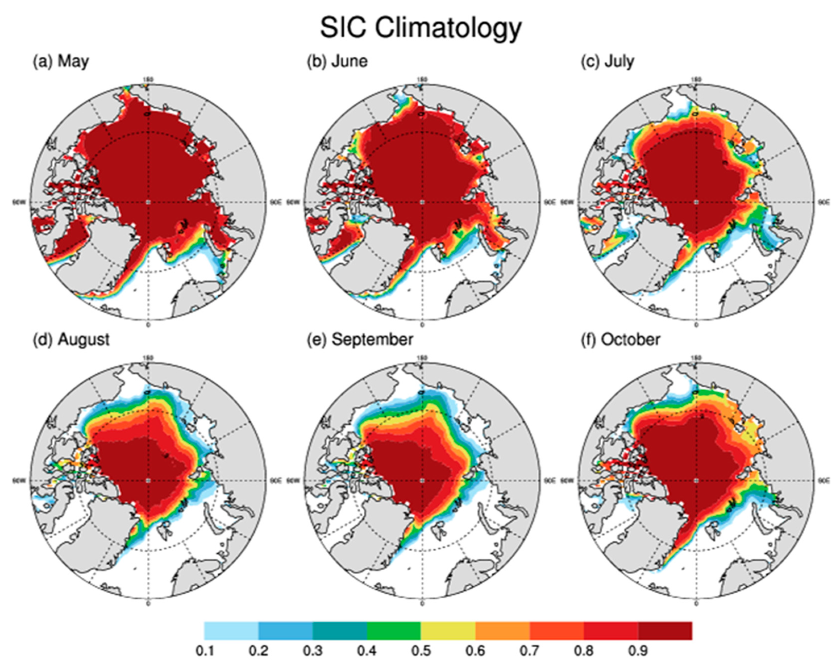
Figure 1. Spatial distribution of the sea ice concentration climatology from May to October (af) for the 39-year period from 1979 to 2017.
Atmosphere 12 00230 g001
Figure 2. Spatial distribution of the sea ice concentration standard deviation from May to October (af) for the 39-year period from 1979 to 2017.
Atmosphere 12 00230 g002
Figure 3. (a) Spatial distribution of the sea ice concentration standard deviation from June to September for the 39-year period from 1979 to 2017. The blue boxes in the map show the key areas of sea ice anomaly variation (centers of large sea ice variability) in different sea areas. (b) The correlation coefficients table of the sea ice indices in different sea areas. **: The coefficient passed the significance t-test at the 99% confidence level.
Atmosphere 12 00230 g003
Figure 4. (a) Key area of sea ice variability in the Barents–Kara Sea; (b) correlation coefficients between sea ice concentration in June, July, August and September; (c) time series of SII in Barents Sea and Kara Sea.
Atmosphere 12 00230 g004
Figure 5. (a) Key area of sea ice variability in the East Siberian Sea and the Laptev Sea; (b) correlation coefficients between sea ice concentration in June, July, August and September; (c) time series of SII in East Siberian Sea and the Laptev Sea.
Atmosphere 12 00230 g005
Figure 6. (a) Key area of sea ice variability in the Beaufort Sea and the Canadian Arctic Archipelago; (b) correlation coefficients between sea ice concentration in June, July, August and September; (c) time series of SII in Beaufort Sea and the Canadian Arctic Archipelago.
Atmosphere 12 00230 g006
Figure 7. The spring sea surface temperature (°C) modes (a,c) and their corresponding time coefficients (b,d) obtained from the PLSR model training for the period 1979–1999, which has best correlation with the Barents–Kara SII.
Atmosphere 12 00230 g007
Figure 8. The evolution of the correlation coefficients distribution between the time series of the first two modes of the PLSR (Figure 7b,d) and the sea surface temperature anomaly (°C) in (a,e) early winter, (b,f) spring, (c,g) summer and (d,h) autumn, for the period 1979–1999. The color area was the area that passed the significance t-test at the 99% (dark) and 95% (light) confidence levels, respectively (Barents–Kara SII).
Atmosphere 12 00230 g008
Figure 9. (a) Lead–lag correlation between the time series of the first two modes of the PLSR and AO index. In the diagram, “−1” represents the previous year, “0” represents this year, and “1” represents the next year. The horizontal dotted line represents the critical line with a statistical confidence level at the 95% level, based on a significant t-test, and the intersection point of the curve and vertical line represents this summer (JJA(0)); (b) regression of the PLSR second mode to SLP (hPa) and 850 hPa U and V wind field (m/s) in the early spring, only drawing a wind field passing the 95% significance t-test.
Atmosphere 12 00230 g009
Figure 10. The spring sea surface temperature (°C) modes (a,c,e) and their corresponding time coefficients (b,d,f) obtained from the PLSR model training for the period 1979–1999, which has best correlation with the East Siberian Sea and the Laptev SII.
Atmosphere 12 00230 g010
Figure 11. The spring sea surface temperature (°C) modes (a,c) and their corresponding time coefficients (b,d) obtained from the PLSR model training for the period 1979–1999, which has best correlation with the Beaufort Sea and the Canadian Arctic Archipelago SII.
Atmosphere 12 00230 g011
Figure 12. The evolution of the correlation coefficients distribution between the time series of the first three modes of the PLSR (Figure 10b,d,f) and the sea surface temperature anomaly (°C) in (a,e,i) early winter, (b,f,j) spring, (c,g,k) summer and (d,h,l) autumn, for the period 1979–1999. The color area was the area that passed the significance t-test at the 99% (dark) and 95% (light) confidence levels, respectively (East Siberian Sea and the Laptev SII).
Atmosphere 12 00230 g012
Figure 13. The evolution of the correlation coefficients distribution between the time series of the first two modes of the PLSR (Figure 7b,d) and the sea surface temperature anomaly (°C) in (a,e) early winter, (b,f) spring, (c,g) summer and (d,h) autumn, for the period 1979–1999. The color area was the area that passed the significance t-test at the 99% (dark) and 95% (light) confidence levels, respectively (Beaufort Sea and the Canadian Arctic Archipelago SII).
Atmosphere 12 00230 g013
Figure 14. Prediction results of the PE PLSR model for the BK index. In the figure, the blue solid line represents the actual SII, the blue solid line is the SII simulated by the model training in 1979–1999, and the red solid line is the SII actually predicted by the model in 2000–2017. Corr1 is the correlation coefficient between the PE PLSR-simulated SII in 1979 and 1999, and Corr2 is the correlation coefficient between the PE PLSR-predicted SII and the actual SII in 2000–2017.
Atmosphere 12 00230 g014
Figure 15. Prediction results of the PE PLSR model for the East Siberian Sea and the Laptev index. In the figure, the blue solid line represents the actual SII, the blue solid line is the SII simulated by the model training in 1979–1999, and the red solid line is the SII actually predicted by the model in 2000–2017. Corr1 is the correlation coefficient between the PE PLSR-simulated SII in 1979 and 1999, and Corr2 is the correlation coefficient between the PE PLSR-predicted SII and the actual SII in 2000–2017.
Atmosphere 12 00230 g015
Figure 16. Prediction results of the PE PLSR model for the Beaufort Sea and the Canadian Arctic Archipelago index. In the figure, the blue solid line represents the actual SII, the blue solid line is the SII simulated by the model training in 1979–1999, and the red solid line is the SII actually predicted by the model in 2000–2017. Corr1 is the correlation coefficient between the PE PLSR-simulated SII in 1979 and 1999, and Corr2 is the correlation coefficient between the PE PLSR-predicted SII and the actual SII in 2000–2017.
Atmosphere 12 00230 g016
Publisher’s Note: MDPI stays neutral with regard to jurisdictional claims in published maps and institutional affiliations.