Satellite-Derived Spatio-Temporal Distribution and Parameters of North Atlantic Polar Lows for 2015–2017

Abstract

A list of North Atlantic polar lows was compiled for 2015–2017. A total of 131 polar lows were found by analyzing the Moderate Resolution Imaging Spectroradiometer (MODIS) infrared imagery and auxiliary information. The study region was additionally divided by the 20° W meridian to assess possible differences in the polar lows occurring in the western and eastern parts of the region. The highest polar low activity was found over the Barents Sea and the northern Norwegian Sea. A large number of polar lows over this region were dual or multiple. When considering such systems as a single event, more polar lows were found in 2015 over the Labrador Sea and southern Davis Strait, which is the region with the second highest number of polar lows. High interannual variability of polar low frequency was noted, which was more pronounced in the western part of the region. During the analyzed period, the largest number of polar lows occurred in January for the western part of the region and in February for the eastern part. The main polar low parameters were similar within the region, with the mean values slightly higher in the western part of the region, but all extreme high values were observed in the eastern part.

1. Introduction

Polar lows are intense maritime mesoscale cyclones occurring over the high latitude ice-free areas [1]. High near-surface wind speeds allow distinguishing them from other polar mesoscale cyclones with 15 m/s often used as a threshold (e.g., [2,3]). Polar lows are characterized by short lifetimes (generally, less than 48 h) and small sizes (generally, less than 600 km), and are often not captured by synoptic charts or atmospheric re-analyses [4,5,6]. Near-surface wind speeds within polar lows may exceed 30 m/s and significant wave height may exceed 10 m [7,8,9]. Polar lows are, thus, certainly dangerous maritime weather events.

Over the years, many studies [10,11,12,13] revealed different mechanisms responsible for polar low development, including the baroclinic instability, conditional instability of the second kind (CISK), and wind-induced surface heat exchange (WISHE). Later, it became apparent that a variety of polar lows exists, referred to as the “polar low spectrum,” which has purely baroclinic systems at one end and purely convective at the other [1]. Consequently, there are different definitions of polar lows and criteria for their identification in different studies. Here, we adopt the widely used definition from Rasmussen and Turner [1], which reads: “A polar low is a small, but fairly intense, maritime cyclone that forms poleward of the main baroclinic zone (the polar front or other major baroclinic zone). The horizontal scale of the polar low is approximately between 200 and 1000 km and surface winds near or above gale force.”

In the Northern Hemisphere, the main polar low genesis regions are the North Pacific Ocean [14] including the Gulf of Alaska and the Bering Sea [15], the Sea of Japan [16], and the North Atlantic, where the highest polar low activity is found [17]. Part of this region, i.e., the Nordic and Barents seas, is most extensively studied. First, climatologies for the region used synoptic charts and only a few satellite images [18,19] and found about 6.5 polar lows per year. Increased availability of satellite data allowed more recent studies to reveal considerably more polar lows. However, the estimates vary greatly (i.e., from about 12 to 45 cases per year) mostly due to the different polar low identification approaches [2,3,20,21].

In contrast, less studies focused on the regions within the North Atlantic west of 20° W. Dedicated studies [22,23] used polar-orbiting and geostationary satellite imagery and reported a relatively high number of polar lows and mesoscale vortices over the eastern Canadian waters with the highest activity over the Labrador Sea and southern Davis Strait. In Kolstad [24], a frequent occurrence of favorable conditions for polar low development was documented, but rather few polar lows (19 in 10 seasons) were found west of 20° W by analyzing the Advanced Very High Resolution Radiometer (AVHRR) quicklook imagery. A slightly higher number of polar lows (10 in 2 years) was found in Blechschmidt [2] for the Irminger Sea by using AVHRR quicklook imagery. This contrasts with the model-based and reanalysis-based objective climatologies, which found polar low activity over the Irminger Sea to be the highest [25] or second highest [17] within the North Atlantic.

In this study, we identify polar lows over the North Atlantic from 2015 to 2017 using a uniform satellite-based method to estimate and intercompare their frequency and parameters within the region, and to produce a polar low list, which might be useful in other polar low-related studies.

2. Data and Methods

The study region includes the North Atlantic Ocean north of 50° N and adjacent parts of the Arctic Ocean, i.e., the Baffin Bay and the Greenland and Barents Seas, which, for brevity, are collectively referred to here as the North Atlantic (Figure 1).

Mesoscale vortices in this region were first identified using the Moderate Resolution Imaging Spectroradiometer (MODIS) thermal infrared imagery (channel 31, 10.78–11.28 µm). Level 1B calibrated radiances with 1-km spatial resolution (MOD021/MYD021) along with the corresponding geolocation products (MOD03/MYD03) were obtained from the NASA’s Level-1 and Atmosphere Archive & Distribution System (LAADS) Distributed Active Archive Center (DAAC) (https://ladsweb.modaps.eosdis.nasa.gov/ (accessed on 28 January 2021)). The MODIS instruments onboard the Terra and Aqua polar orbiting satellites provide almost uniform coverage of the northern areas of the study region (i.e., Barents Sea, northern Norwegian and Greenland Seas) as consecutive satellite swaths for a certain area are separated by no more than about 1 h 40 min with only one temporal gap between the swaths per day, which does not exceed 4 h. However, for more southern latitudes (i.e., <65° N), there are two 6–8 h gaps between the available data per day. Hence, the AVHRR channel 4 quicklook infrared imagery from the MetOp-B and NOAA-19 satellites provided by the Dundee Satellite Receiving Station at the University of Dundee (presently, Dundee Satellite Station Ltd. Dundee, UK) was additionally used to better assess the development and displacement of a system in question when they were uncertain. However, this did not considerably reduce the gaps (generally, by about only 1 h) as the ground tracks of the MetOp-B and NOAA-19 satellites were close in space and time to those of the Terra and Aqua satellites, respectively. AVHRR imagery was thus not used in the construction of polar low tracks or estimation of their parameters.

Maximum near-surface wind speeds within the identified mesoscale vortices were estimated using the data from the Advanced Scatterometer (ASCAT) instrument onboard the MetOp-A and MetOp-B satellites. Level 2 wind vectors with 12.5-km spatial resolution were obtained from the NASA’s Physical Oceanography DAAC (https://podaac.jpl.nasa.gov/ (accessed on 28 January 2021)). Exceedance of the 15 m/s threshold at least once during lifetime was required for a system to be further considered as a polar low. Examples of the identified polar lows over the Labrador and Barents Seas are shown in Figure 2. The accuracy of the ASCAT wind speed data, which is about 1 m/s [26], is only of concern in borderline cases, where it could impact the decision whether to include or dismiss the case. To mitigate the possibility of the incorrect inclusion of cases, the wind speed threshold was required to be exceeded in at least four adjacent grid cells. There is, however, a possibility of wind speed underestimation leading to the incorrect omission of cases.

The methodology described above could, however, lead to the inclusion of numerous small-scale extratropical cyclones, which may appear similar to polar lows on infrared imagery [1,20]. To better distinguish polar lows from other systems, it is, therefore, necessary to assess the development mechanisms of the analyzed cyclones. For this purpose, we used surface synoptic charts produced by the Met Office and Deutscher Wetterdienst along with the European Centre for Medium-Range Weather Forecasts (ECMWF) fifth generation reanalysis ERA5 [27] data, which included mean sea level pressure, air temperature at 2 m and at 850 hPa, and geopotential at 500 and 1000 hPa. Joint analysis of these data with the available infrared imagery allowed excluding frontal systems following the classical Norwegian or Shapiro-Keyser cyclone models and retaining polar lows, which generally develop during cold air outbreaks along low-level baroclinic zones and are triggered by the positive vorticity advection supplied by upper-level cold lows or troughs.

The tracks of all identified polar lows were constructed by recording the locations of polar low centers on successive MODIS swaths. Polar low center locations were set to the cloud-free eye or, if not present, to the circulation center determined by the rotation of the system on successive infrared images when possible, or subjectively identified considering previous track points, the overall movement of the system, and smoothness of the resulting track. The number of track points per polar low in the resulting dataset spans from 2 (only one case) to 59 (only one case as well) with the median number of track points being 8.

Main polar low parameters were calculated as follows. The polar low diameter was approximated by averaging the lengths of two roughly orthogonal lines crossing the main cloud structure (excluding the cloud tail when present). The reported values are maximum diameters reached during the cyclone mature stage. Lifetimes were calculated as the difference between the last and the first MODIS observation of a given polar low. Distance travelled is the sum of distances between consecutive track points. Translation speed is the total distance travelled divided by the lifetime. Maximum wind speed refers to the maximum value of near-surface wind speed reached within a polar low lifetime. To ensure that only the values within a given polar low are considered and not those belonging to, e.g., large-scale synoptic fields or adjacent mesocyclones or polar lows in the case of multiple systems, and to eliminate the possible effect of retrieval errors, the maximum wind speed was determined manually by relating the ASCAT wind speed fields rounded down and plotted as integers with a 1-m/s step and MODIS imagery and then selecting the lowest value within a group of at least four adjacent grid cells with maximum wind speeds within the polar low area. Dominant propagation direction was approximated first by binning the track segments of a given polar low into 30° bins and then selecting the bin with the longest total duration of track segments within it.

Dual and multiple polar lows refer to the cases when two or more polar lows formed within the same synoptic environment in proximity to each other and were simultaneously active during any time period. Total polar low numbers are given both when considering such systems as a single event and when counting each system individually.

3. Results and Discussion

3.1. Temporal Distribution

Overall, 131 polar lows were found over the North Atlantic for 2015–2017. The largest number of polar lows (61) was found in 2015, 45 polar lows were identified in 2017, and only 25 cases occurred in 2016 (

Table 1. Temporal distribution of identified polar lows. Numbers in brackets are obtained when considering dual and multiple polar lows as a single event.

Polar Lows		Jan	Feb	Mar	Apr	Oct	Nov	Dec	Total
All	2015	15 (12)	16 (11)	6 (5)	1	1	7 (4)	15 (8)	61 (42)
	2016	5 (3)	0	5 (2)	4 (3)	0	4 (2)	7 (5)	25 (15)
	2017	8 (6)	15 (9)	8 (5)	3	0	6 (5)	5 (4)	45 (32)
	Total	28 (21)	31 (20)	19 (12)	8 (7)	1	17 (11)	27 (17)	131 (89)
≤20° W	2015	9	6 (5)	3	1	0	4 (3)	4 (3)	27 (24)
	2016	3 (1)	0	0	0	0	0	2	5 (3)
	2017	1	2	1	2	0	1	3 (2)	10 (9)
	Total	13 (11)	8 (7)	4	3	0	5 (4)	9 (7)	42 (36)
>20° W	2015	6 (3)	10 (6)	3 (2)	0	1	3 (1)	11 (5)	34 (18)
	2016	2	0	5 (2)	4 (3)	0	4 (2)	5 (3)	20 (12)
	2017	7 (5)	13 (7)	7 (4)	1	0	5 (4)	2	35 (23)
	Total	15 (10)	23 (13)	15 (8)	5 (4)	1	12 (7)	18 (10)	89 (53)

). Hereinafter, the study region is additionally divided by the 20° W meridian to assess possible differences in the polar lows occurring in the western (mostly corresponding to the Davis Strait and Labrador and Irminger Seas) and eastern (mostly corresponding to the more studied Nordic and Barents seas) parts of the region. Accordingly, polar lows, which formed west (east) of 20° W, are referred to as western (eastern) polar lows.

A total of 89 polar lows were found over the eastern region including 34 that occurred in 2015, 20 that occurred in 2016, and 35 that occurred in 2017. The interannual variability is even higher in the western region, where 27 polar lows formed in 2015, 5 polar lows formed in 2016, and 10 formed in 2017 (42 in total). There is a considerably higher number of dual and multiple polar lows in the eastern region. If such cases are counted as a single event, the difference in the number of polar lows between the regions is reduced, i.e., there are 36 events over the western and 53 events over the eastern region. Moreover, more polar low events were found over the western region (24) than over the eastern (18) in 2015.

The mean annual number of eastern polar lows obtained here (about 30) lies within the range found in the literature. In particular, about 45 polar lows per year are found on average in Smirnova et al. [3]. Some of this difference may possibly be attributed to the different data used and to the large interannual variability of polar low frequency, which certainly affects the robustness of our estimates due to the rather short period analyzed. Another source of this difference is that no additional information was used in Smirnova et al. [3] to analyze the development mechanisms of selected systems, which might have led to the selection of smaller extratropical cyclones or other vortices that would not be considered polar lows in the present study. In contrast, lower mean annual numbers are found in Noer et al. [20] and Rojo et al. [21]. We find that their updated dataset [28] contains 21 cases on average for the same years as analyzed here (2015–2017). Some of this difference is most likely because our list contains more minor cases as in the present study we did not consider the magnitude of wind speed exceedance within a cyclone relatively to the ambient wind speed field as a selection criterion and could possibly include cases with less magnitude than would be required in these studies.

Although identification was performed for all months, no polar lows were found from May to September, and only one was found in October (Figure 3). On average, for the western region, the largest number of polar lows is observed in January. For the eastern region, more polar lows were found in February. Monthly polar low frequencies are also highly variable, e.g., no polar lows were observed in February 2016. Longer-term satellite-derived polar low climatologies for the Nordic and Barents seas find maximum polar low frequency in March [3,21]. However, if we compare our results to the updated dataset by Rojo et al. [28], which includes more recent years, we find a similar monthly distribution for 2015–2017 to the one obtained here, with a clear February maximum.

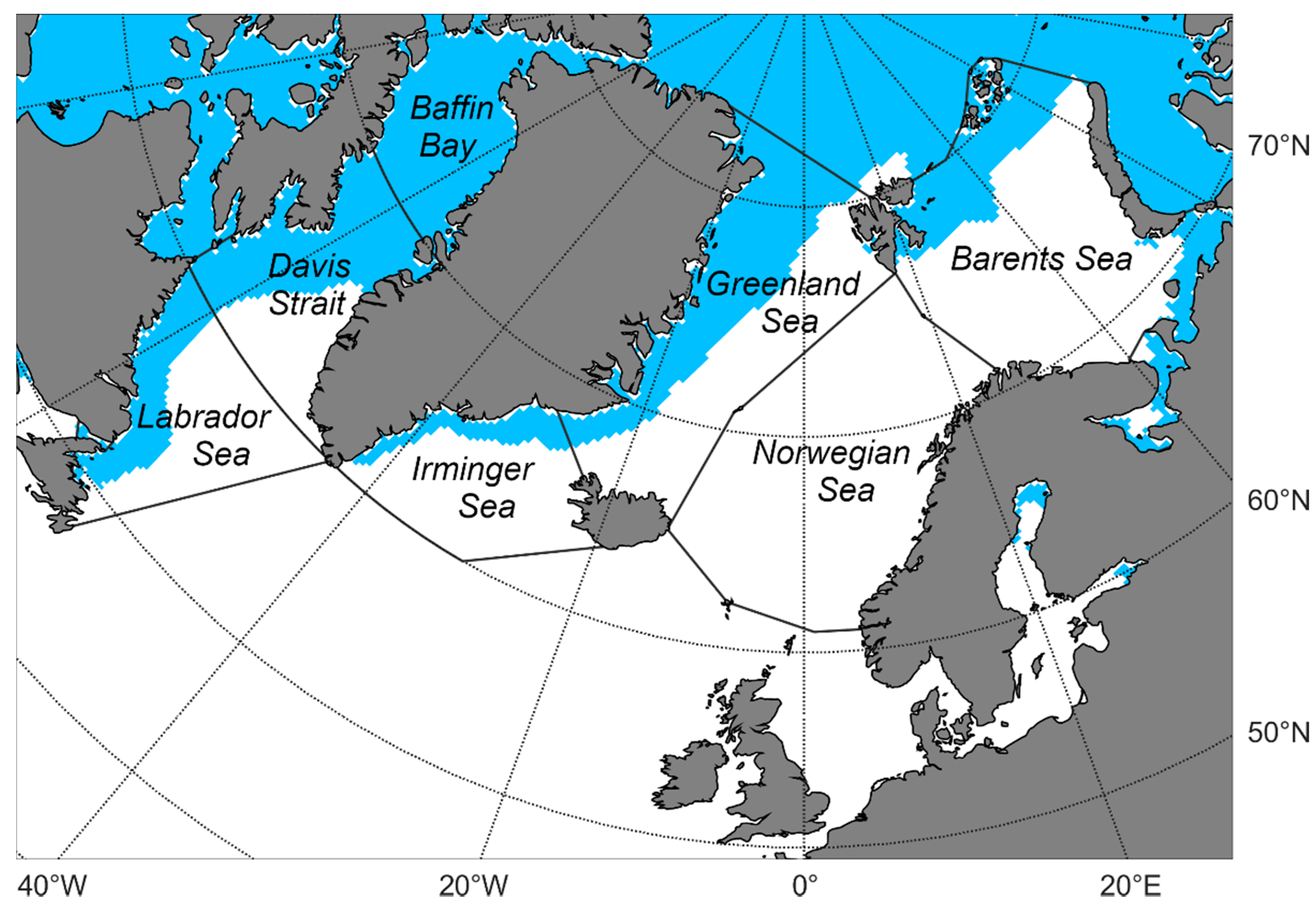
3.2. Spatial Distribution

Tracks of all identified polar lows are plotted in Figure 4. The highest polar low activity is observed in the region encompassing the Barents Sea and northern Norwegian Sea (north of 70° N), where more than half of identified polar lows (68) originated. This is in line with other studies, which reported peak polar low numbers within this region [3,20,21]. At the same time, these studies also found a high number of polar lows over the Norwegian Sea south of 70° N, where, rather surprisingly, very few polar lows (8) are observed here. This may be due to the high variability of polar low frequency and formation locations, which depend on the large-scale circulation patterns (e.g., [21,29]).

Another region with high polar low activity is found over the Labrador Sea and southern Davis Strait where 28 cyclones formed. Similar to the Nordic and Barents seas, this region is prone to frequent cold air outbreaks and is located close to one of the low-pressure centers within the circumpolar vortex providing the upper-level forcing necessary for polar low development [1]. Using the indices representing static stability and upper-level forcing, Kolstad [24] found that the favorable conditions for polar low development are observed in the Labrador Sea even more often than in the Nordic and Barents seas, although the lower sea surface temperatures in the Labrador Sea may be a factor decreasing the probability of polar low formation. If we consider the dual and multiple polar lows as a single event, which better characterizes the frequency of the environmental conditions that led to polar low formation regardless of one or several cyclones developed within this environment, the difference between the regions with the highest polar low activity decreases, i.e., 24 polar low events occurred over the Labrador Sea and southern Davis Strait and 36 over the Barents Sea and northern Norwegian Sea. Furthermore, in 2015, more polar low events occurred over the Labrador Sea and southern Davis Strait (15) than over the Barents Sea and northern Norwegian Sea (11). Analyzing the influence of large-scale atmospheric circulation on polar low formation, the positive phase of the North Atlantic Oscillation (NAO) was found to set favorable conditions for polar low development over the western North Atlantic promoting colder temperatures, lower 500 hPa geopotential heights and northerly (for the Davis Strait), westerly (for the Labrador Sea), and northerly to northeasterly (for the Irminger Sea) flows inducing cold air outbreaks, and unfavorable conditions over the Norwegian and Barents Sea, where southerly to southwesterly flows are promoted, which prevents cold air outbreaks [29,30]. Indeed, our results likely reflect this since using the values provided by the NOAA Climate Prediction Center [31], we find that the average monthly mean NAO index for the colder months (January-April and October-December) of 2015 is 1.39, i.e., a strongly positive NAO phase, while less pronounced, albeit also positive values are found for 2016 and 2017 (0.51 and 0.72, respectively), which presumably implies that other weather regimes were prevalent for more extended periods during these years.

High polar low activity over the Irminger Sea found in the model-based or reanalysis-based objective climatologies (e.g., [17,25]) is not present in our results. Only nine polar lows were identified over this region including seven that occurred in 2015 and two that occurred in 2017. This difference might also be attributed to the more positive NAO phase in 2015. We note, however, a large number of small extratropical cyclones and mesoscale vortices within this region. Some of the latter had wind speeds exceeding the 15 m/s threshold, but, nevertheless, were not included since, as far as we could ascertain, their development differed from that expected for polar lows, e.g., there was no upper-level forcing or wind speeds exceeding 15 m/s were only on periphery and were considered to belong to synoptic flow.

No polar lows were found over the Baffin Bay, which is mostly ice-covered throughout the cold season. During the analyzed period, freeze-up, on average, started in late October and a small ice-free area near Greenland could be observed until mid-December.

3.3. Polar Low Parameters

The distribution of polar lows by diameter is shown in Figure 5a. Most polar lows (60%) have maximum diameters at mature stage that are in the 200–400 km range. Diameters of only six polar lows exceeded 600 km, all in the eastern region, and one of them exceeded 700 km. Smaller polar lows with less than 200-km diameters account for 15% of cases. Such small systems are more frequent in the eastern region, where 20% fall into this category. Overall, western polar lows are slightly larger than eastern ones with more cases in the 300–600-km range. The mean diameter is 351 km for western and 321 km for eastern polar lows. This difference might be due to the considerably higher number of multiple systems in the eastern region, which can be rather small (e.g., several minor, smaller polar lows may accompany a major, larger polar low), but the mean diameter of eastern polar lows only grows by 10 km when neglecting multiple systems.

Figure 5b shows the distribution of polar lows by lifetime. Most polar lows (56%) existed for less than 24 h and 26% are in the 12–18 h range. The maximum recorded polar low lifetime is 102 h. Western polar lows generally existed slightly longer than eastern ones with the mean lifetimes of 20.6 h and 19.6 h, respectively, although all the longest-lived systems (more than 42 h) were found in the eastern region. Since almost all western polar lows originated south of 65° N latitude, the local minima at 18–24 h and 30–36 h lifetimes are most likely due to the decreased temporal resolution of MODIS imagery at lower latitudes.

Distance travelled is also generally larger for western polar lows (Figure 5c). Almost 30% of them travelled 500–750 km. For eastern polar lows, 37% are in the 250–500 km range. The mean values are 625 and 569 km for western and eastern polar lows, respectively. There are nine cases in total when polar lows travelled more than 1500 km, two of which travelled more than 2000 km (both in the eastern region).

Polar low translation speeds are similar in both regions (Figure 5d). About 30% of cases are in the 6–9 m/s range. Seven polar lows exceeded the translation speed of 18 m/s, and the fastest moving one reached 21 m/s. The mean values are 8.8 m/s for the western region and 8.9 m/s for the eastern region.

As mentioned above, the maximum wind speeds were determined by rounding down the ASCAT data and recording integers with a 1 m/s step. Since exact decimal values were unknown, they were approximated by adding 0.5 m/s to each recorded wind speed value. The resulting distribution of polar lows by maximum wind speed is shown in Figure 6. As for most other parameters, generally larger values are found for the western polar lows. About 40% of them have wind speeds in the 19–21 m/s range. More than half of the eastern polar lows are in the 17–21 m/s range. The mean wind speed is 21 m/s for the western polar lows and 20 m/s for the eastern polar lows. Only two polar lows were found to exceed 27 m/s wind speed, one of which exceeded 28 m/s wind speed.

Figure 7 shows the distribution of polar lows by dominant propagation direction. More than half of the western polar lows propagate predominantly eastwards and about one-third propagate northeastward or southeastward. The eastern polar lows predominantly propagate southward or southeastward.

3.4. Formation Conditions

The large-scale synoptic environment during the formation of western and eastern polar lows may be assessed using Figure 8, which shows composites of 500-hPa geopotential height (Z500) anomalies and 925-hPa wind vectors. The composites were obtained from ERA5 data using the closest 1-h time step to the first observation of each polar low in our list. Anomaly of Z500 represents the difference between Z500 at a given time step and the mean Z500 for October–April 2015–2017.

For the western polar lows, there is a strong negative anomaly centered above southern Greenland and covering the Labrador Sea, the Davis Strait, and the Irminger Sea (Figure 8a). The largest anomaly magnitude exceeds -200 m, which confirms the presence of strong upper-forcing during formation of the identified polar lows. Lower-level winds indicate the presence of cold-air outbreaks as intense northeasterly and easterly flows advect the colder air located over the continent and sea ice toward the warmer sea surface of the Davis Strait and Labrador Sea. During formation of the western polar lows, generally unfavorable conditions for polar low development are found in the eastern region, with small, albeit negative, Z500 anomalies and weak southwesterly to southeasterly flow. Rather favorable conditions are found over the Greenland Sea closer to the Greenland coast, but sea ice in this region suppresses any possible developments.

Similarly, during the formation of the eastern polar lows, a strong negative Z500 anomaly is observed over the area of the highest polar low activity in the eastern region (Figure 8b). This anomaly is centered over the Barents Sea and has the largest magnitudes exceeding −180 m. Strong northerly to north-easterly flow leads to the outbreaks of cold Arctic air over the region. During this situation, unfavorable conditions for polar low formation are found in the western region, where a weak positive anomaly is present and only a minor cold air flow may be observed over the Davis Strait and northwestern Labrador Sea.

Overall, slightly weaker negative Z500 anomaly and lower-level flow are found during formation of the eastern polar lows compared to the conditions during formation of the western polar lows. The distributions in Figure 8 are in excellent agreement with those presented in Mallet et al. [29] for Noer et al. [20] and Kolstad [24] polar low lists.

Another view of polar low formation conditions is presented in Figure 9, which shows the composites of the main parameters within a 500-km radius centered around each polar low. Same as above, the closest in time to the first polar low observation ERA5 data were used for these composites.

Figure 9a,d show composites of the difference between the sea surface (θ_SST) and 500 hPa (θ₅₀₀) potential temperatures for the western and eastern regions. The differences between the sea surface or skin temperature or potential temperature and that at a higher level are often used to characterize atmospheric static stability and identify marine cold air outbreaks (e.g., [17,32,33]). Stoll et al. [17] found that the difference between the sea surface and 500-hPa potential temperatures performs better than other similar criteria. In Figure 9a,d, higher values indicate less stable atmosphere, and the highest values are found within 100 km of polar low centers in both regions. The magnitude of the θ_SST−θ₅₀₀ difference is similar between the regions, except for the area of the highest values, exceeding −5 K, which is considerably larger in the western region. The highest values are approximately located at the northwestern sector for the western polar lows and at the northeastern sector for the eastern polar lows, likely reflecting the orientations of the upper-level troughs present in Z500 composite fields (Figure 9c,f). Figure 9b,e show composites of 850-hPa air temperature (T850). Strong baroclinic environments are evident, as the largest temperature gradients are about 2 K over 100 km with colder air located in the west and north-northwest for the western and eastern polar lows, respectively.

4. Conclusions

In this study, polar lows over the North Atlantic were identified in MODIS infrared imagery and their intensity was assessed using ASCAT scatterometer data. The development of selected systems was examined using synoptic surface charts and atmospheric reanalysis data to better exclude smaller extratropical cyclones or more minor vortices. A total of 131 polar lows were found for 2015–2017. The number of polar lows over the eastern part of the study region (>20° W) is 89, which is more than two times higher than for the western part (<20° W), where 42 polar lows were found. A substantial part of this difference is due to the larger number of dual or multiple polar lows over the eastern region. When considering them as a single event, the difference is markedly decreased, i.e., there are 53 events in the eastern region and 36 events in the western region.

Most of the identified polar lows (68) originated over the Barents Sea and northern Norwegian Sea (north of 70° N). The second highest number of polar lows (28) formed over the Labrador Sea and southern Davis Strait. Counting dual and multiple systems as a single event results in a decreased difference as well. In particular, more polar low events occurred over the Labrador Sea and southern Davis Strait than over the Barents Sea and northern Norwegian Sea in 2015. This is likely a consequence of a strongly positive NAO phase in the colder months of 2015, during which the number of polar lows is increased over the Labrador Sea and decreased over the Norwegian and Barents Sea [29,30].

Overall, polar low frequency exhibits high interannual variability, which was noted in many studies (e.g., [3,20,21]). In particular, in the present study, 61, 25, and 45 polar lows were found in 2015, 2016, and 2017, respectively. Some of this variability might be due to the variation of the large-scale atmospheric circulation patterns (e.g., [21,29]). For instance, the strong dependence of the western polar low frequency on the NAO phase found in previous studies [29,30,34] with more events occurring during the positive NAO phase, have likely influenced the numbers we obtained for this region as indicated by our simplified estimates using the average values of the monthly mean NAO index for colder months.

Overall, during the analyzed period, more polar lows were observed in February, while for the western region the maximum number was found in January. The monthly distribution is, however, highly variable, as found in previous studies (e.g., [3,21]) and also here (e.g., no polar lows were identified in February 2016). The distributions of polar lows by their main parameters derived here for the North Atlantic generally agree with those previously reported for polar lows over the Nordic and Barents seas (e.g., [3,21]). The following mean values for the main polar low parameters were obtained: diameter of 331 km, lifetime of 19.9 h, distance travelled of 587 km, translation speed of 8.9 m/s, and wind speed of 20.3 m/s. Comparing the mean values for the two subregions, except for the mean translation speeds, which are almost equal, higher mean values were found for the western polar lows, although the difference is rather small. In particular, the mean diameter and distance travelled are larger by about 10%, mean lifetime is longer by 1 h, and mean wind speed is higher by 1 m/s. At the same time, all extreme high values of these parameters are observed in the eastern region. The estimated dominant polar low propagation directions are mostly westward for the western polar lows and mostly southward and southwestward for the eastern polar lows.

Given the high interannual variability in polar low frequency and formation locations and our quite limited study period, we certainly do not consider the derived polar low spatio-temporal distributions as robust in the sense that they would hold for other years. Rather, they are only intended to reflect the polar low activity during the period analyzed here. The polar low list compiled here (Table S1) might also be useful for other polar low-related studies and might be extended in the future.

References

1. Rasmussen, E.A.; Turner, J. Polar Lows: Mesoscale Weather Systems in the Polar Regions; Cambridge University Press: Cambridge, UK, 2003. [Google Scholar]
2. Blechschmidt, A.-M. A 2-year climatology of polar low events over the Nordic seas from satellite remote sensing. Geophys. Res. Lett. 2008, 35, L09815. [Google Scholar] [CrossRef]
3. Smirnova, J.E.; Golubkin, P.A.; Bobylev, L.P.; Zabolotskikh, E.V.; Chapron, B. Polar low climatology over the Nordic and Barents seas based on satellite passive microwave data. Geophys. Res. Lett. 2015, 42, 5603–5609. [Google Scholar] [CrossRef] [Green Version]
4. Laffineur, T.; Claud, C.; Chaboureau, J.P.; Noer, G. Polar lows over the Nordic Seas: Improved representation in ERA-Interim compared to ERA-40 and the impact on downscaled simulations. Mon. Weather Rev. 2014, 142, 2271–2289. [Google Scholar] [CrossRef]
5. Zappa, G.; Shaffrey, L.; Hodges, K. Can polar lows be objectively identified and tracked in the ECMWF operational analysis and the ERA-Interim reanalysis? Mon. Weather Rev. 2014, 142, 2596–2608. [Google Scholar] [CrossRef]
6. Smirnova, J.; Golubkin, P. Comparing polar lows in atmospheric reanalyses: Arctic System Reanalysis versus ERA-Interim. Mon. Weather Rev. 2017, 145, 2375–2383. [Google Scholar] [CrossRef]
7. Orimolade, A.P.; Furevik, B.R.; Noer, G.; Gudmestad, O.T.; Samelson, R.M. Waves in polar lows. J. Geophys. Res. Oceans 2016, 121, 6470–6481. [Google Scholar] [CrossRef]
8. Golubkin, P.; Kudryavtsev, V.; Smirnova, J.; Chapron, B. Abnormal Waves Generated by Polar Lows: Evaluation of Expectancy. In Proceedings of the 2018 IEEE International Geoscience and Remote Sensing Symposium, Valencia, Spain, 22–27 July 2018; pp. 3286–3289. [Google Scholar]
9. Rojo, M.; Claud, C.; Noer, G.; Carleton, A.M. In situ measurements of surface winds, waves, and sea state in polar lows over the North Atlantic. J. Geophys. Res. Atmos. 2019, 124, 700–718. [Google Scholar] [CrossRef] [Green Version]
10. Harrold, T.W.; Browning, K.A. The polar low as a baroclinic disturbance. Q. J. R. Meteorol. Soc. 1969, 95, 710–723. [Google Scholar] [CrossRef]
11. Rasmussen, E. The polar low as an extratropical CISK disturbance. Q. J. R. Meteorol. Soc. 1979, 105, 531–549. [Google Scholar] [CrossRef]
12. Emanuel, K.A.; Rotunno, R. Polar lows as arctic hurricanes. Tellus A 1989, 41, 1–17. [Google Scholar] [CrossRef]
13. Montgomery, M.T.; Farrell, B.F. Polar low dynamics. J. Atmos. Sci. 1992, 49, 2484–2505. [Google Scholar] [CrossRef] [Green Version]
14. Yarnal, B.; Henderson, K.G. A climatology of polar low cyclogenetic regions over the North Pacific Ocean. J. Clim. 1989, 2, 1476–1491. [Google Scholar] [CrossRef] [Green Version]
15. Businger, S. The synoptic climatology of polar-low outbreaks over the Gulf of Alaska and the Bering Sea. Tellus A 1987, 39, 307–325. [Google Scholar] [CrossRef] [Green Version]
16. Yanase, W.; Niino, H.; Watanabe, S.I.; Hodges, K.; Zahn, M.; Spengler, T.; Gurvich, I.A. Climatology of polar lows over the Sea of Japan using the JRA-55 reanalysis. J. Clim. 2016, 29, 419–437. [Google Scholar] [CrossRef]
17. Stoll, P.J.; Graversen, R.G.; Noer, G.; Hodges, K. An objective global climatology of polar lows based on reanalysis data. Q. J. R. Meteorol. Soc. 2018, 144, 2099–2117. [Google Scholar] [CrossRef] [Green Version]
18. Wilhelmsen, K. Climatological study of gale-producing polar lows near Norway. Tellus A 1985, 37, 451–459. [Google Scholar] [CrossRef]
19. Ese, T.; Kanestrøm, I.; Pedersen, K. Climatology of polar lows over the Norwegian and Barents Seas. Tellus A 1988, 40, 248–255. [Google Scholar] [CrossRef]
20. Noer, G.; Saetra, Ø.; Lien, T.; Gusdal, Y. A climatological study of polar lows in the Nordic Seas. Q. J. R. Meteorol. Soc. 2011, 137, 1762–1772. [Google Scholar] [CrossRef]
21. Rojo, M.; Claud, C.; Mallet, P.E.; Noer, G.; Carleton, A.M.; Vicomte, M. Polar low tracks over the Nordic Seas: A 14-winter climatic analysis. Tellus A 2015, 67, 24660. [Google Scholar] [CrossRef]
22. Hanley, D.; Richards, W.G. Polar Lows in Canadian Waters 1977–1989; Report: MAES 2-91; Scientific Services Division, Atlantic Region, Atmospheric Environment Service: Toronto, ON, Canada, 1991. [Google Scholar]
23. Parker, N. Cold Air Vortices and Polar Low Handbook for Canadian Meteorologists; Environment Canada: Edmonton, AB, Canada, 1997.
24. Kolstad, E.W. A global climatology of favourable conditions for polar lows. Q. J. R. Meteorol. Soc. 2011, 137, 1749–1761. [Google Scholar] [CrossRef]
25. Zahn, M.; von Storch, H. A long-term climatology of North Atlantic polar lows. Geophys. Res. Lett. 2008, 35. [Google Scholar] [CrossRef] [Green Version]
26. Vogelzang, J.; Stoffelen, A.; Verhoef, A.; Figa-Saldaña, J. On the quality of high-resolution scatterometer winds. J. Geophys. Res. Oceans 2011, 116. [Google Scholar] [CrossRef] [Green Version]
27. Hersbach, H.; Bell, B.; Berrisford, P.; Hirahara, S.; Horányi, A.; Muñoz-Sabater, J.; Nicolas, J.; Peubey, C.; Radu, R.; Schepers, D.; et al. The ERA5 global reanalysis. Q. J. R. Meteorol. Soc. 2020, 146, 1999–2049. [Google Scholar] [CrossRef]
28. Rojo, M.; Noer, G.; Claud, C. Polar Low Tracks in the Norwegian Sea and the Barents Sea from 1999 until 2019; PANGAEA: Bremen, Germany, 2019. [Google Scholar] [CrossRef]
29. Mallet, P.E.; Claud, C.; Cassou, C.; Noer, G.; Kodera, K. Polar lows over the Nordic and Labrador Seas: Synoptic circulation patterns and associations with North Atlantic-Europe wintertime weather regimes. J. Geophys. Res. Atmos. 2013, 118, 2455–2472. [Google Scholar] [CrossRef]
30. Claud, C.; Duchiron, B.; Terray, P. Associations between large-scale atmospheric circulation and polar low developments over the North Atlantic during winter. J. Geophys. Res. Atmos. 2007, 112. [Google Scholar] [CrossRef] [Green Version]
31. NOAA Climate Prediction Center—Teleconnections: North Atlantic Oscillation. Available online: https://www.cpc.ncep.noaa.gov/products/precip/CWlink/pna/nao.shtml (accessed on 14 December 2020).
32. Kolstad, E.W.; Bracegirdle, T.J.; Seierstad, I.A. Marine cold-air outbreaks in the North Atlantic: Temporal distribution and associations with large-scale atmospheric circulation. Clim. Dyn. 2009, 33, 187–197. [Google Scholar] [CrossRef]
33. Papritz, L.; Spengler, T. A Lagrangian climatology of wintertime cold air outbreaks in the Irminger and Nordic Seas and their role in shaping air–sea heat fluxes. J. Clim. 2017, 30, 2717–2737. [Google Scholar] [CrossRef]
34. Carleton, A.M. Meridional transport of eddy sensible heat in winters marked by extremes of the North Atlantic Oscillation, 1948/49–1979/80. J. Clim. 1988, 1, 212–223. [Google Scholar] [CrossRef] [Green Version]
Figure 1. The study region and the main areas within it. The blue shaded area denotes the median cold season (October-April) sea ice extent for 2015–2017.
Atmosphere 12 00224 g001
Figure 2. Examples of polar lows identified in MODIS infrared imagery with ASCAT near-surface wind speeds overlayed. (a) 1 March 2017. (b) 11 March 2017.
Atmosphere 12 00224 g002
Figure 3. Monthly distribution of polar lows. Total bar lengths correspond to all observed polar lows. Darker colored bar bases represent the numbers obtained when considering dual and multiple polar lows as a single event.
Atmosphere 12 00224 g003
Figure 4. Tracks of identified polar lows. Circles represent locations of the first observation of a given polar low color-coded according to the years the cyclones occurred. Lines represent median sea ice extent during colder months (January-April, October-December) of the analyzed years.
Atmosphere 12 00224 g004
Figure 5. Distribution of polar lows by (a) diameter, (b) lifetime, (c) distance travelled, and (d) translation speed.
Atmosphere 12 00224 g005
Figure 6. Distribution of polar lows by maximum near-surface wind speed reached during their lifetimes.
Atmosphere 12 00224 g006
Figure 7. Distribution of polar lows by dominant propagation direction. The radial axes represent the proportion of polar lows (%).
Atmosphere 12 00224 g007
Figure 8. Composite of 500-hPa geopotential height anomaly (m, shaded) and 925-hPa wind vectors (arrows) during formation of (a) western and (b) eastern polar lows.
Atmosphere 12 00224 g008
Figure 9. Composites within a 500-km radius of polar low centers of (a), (d) difference between the sea surface and 500-hPa potential temperatures, (b, e) temperature at 850 hPa and (c, f) geopotential height at 500 hPa for (ac) western and (df) eastern polar lows.
Atmosphere 12 00224 g009