Representativeness of Carbon Dioxide Fluxes Measured by Eddy Covariance over a Mediterranean Urban District with Equipment Setup Restrictions

Abstract

The CO₂ fluxes measured by the eddy covariance technique (EC) are presented for a district of the urban area of Bari (Italy). The applicability of the EC method was satisfied even though the measurements were taken at a limited height. The CO₂ fluxes are representative of an area with public offices and schools, the university campus, green areas, and busy roads with intensive traffic during school and office times. The measurements were carried out in March–June, covering late winter, characterized by huge vehicle traffic and domestic heating, until late spring, characterized by reduced activities for schools and the university. The source area was determined as a function of atmospheric stability, for data with the ratio between measurement-height/buildings-height in the range of 1.3–1.5. The measured CO₂ fluxes were compared to gas consumption values. The results show that the district is a strong source of CO₂ during the winter. Emissions were drastically reduced (−82%) after the heating was switched off, and a further decrease in CO₂ emissions (−50%) occurred with the reduction of school activities, partly due to the mitigating effect of green areas with large trees in the area.

1. Introduction

Many experimental studies are available for understanding the role of human activities on atmospheric carbon dioxide (CO₂) dynamics in urban ecosystems. These works are mostly based on measurements of CO₂ fluxes by the eddy-covariance (EC) technique [1] at different urban locations all over the world. In general, the influence of human activities on urban CO₂ fluxes has been identified in three specific sources/sinks: (i) Fossil fuel and gas combustions for heating and electricity, (ii) urban traffic, and (iii) biogenic emission and uptake from vegetation. Furthermore, local weather has a major influence on CO₂ exchanges at urban ecosystem level (in terms of air temperature and humidity, wind speed and direction, solar radiation, and rain).

CO₂ fluxes are measured mainly in America and Europe (see [2] for a review), and in more recent years in Asia (e.g., [3]). In general, intensity and distribution of CO₂ sources and sinks in urban ecosystems are clearly and strongly seasonal, as domestic heating is linked to air temperature and humidity; urban traffic is linked to day-of-the-week and rush hour; vegetation cover is related to the plant growth cycle, which in turn is affected by the thermodynamics of the biosphere. Urban CO₂ fluxes therefore change with changing seasons. Velasco et al. [4] carried out measurements during and after holidays for 23 days, finding that CO₂ fluxes followed a diurnal pattern, correlated with traffic and urban land use (scholar, residential, and commercial areas). Moreover, effects of extension and location of the EC tower were found for coastal (Melbourne, [5]) and semi-arid areas in the USA [2]. Among many others, similar behaviors of CO₂ fluxes were found in several contrasting urban sites like Edinburgh [6], Chicago [7], Tokyo [8], Helsinki [9], Mexico City [10], London [11], Łódź [12], Beijing [13], and Basel [14].

Even though the Mediterranean region has been identified as one of the most prominent “hot-spots” in future climate change projections, with a delicate equilibrium between inner rural, suburban, and coastal areas [15,16], the studies on CO₂ fluxes in urban sites of this region are rare. By analyzing the urban heating and traffic, Matese et al. [17] found that in Florence (Central Italy) the CO₂ Net Ecosystem Exchange is well related to the seasonal changes of air temperature. Same results were found for Rome (Central Italy, [18]) subject to Mediterranean climate, warm and temperate, and Lecce (Southern Italy, [19]), a city quite far from the sea and subject to a semi-arid climate. In a coastal Mediterranean big city such as Marseille, Grimmond et al. [20] showed that a central district is almost always a CO₂ source, but the vegetation reduces the magnitude of the CO₂ emissions when the wind comes from the green areas inland (during the afternoon).

Matching the requirements for EC measurements above urban areas can be complex. In fact, the great patchiness of the urban surface, usually a mixture of building, asphalt/concrete roads and vegetation, translates into complex roughness characteristics, making it challenging for EC measurements, and for drawing conclusions in terms of representativeness at district or city scales [21]. In particular, the EC instrumentation should be installed at a tower height greater than the blending height (defined as the scale at which the flow changes from equilibrium with the local surface to horizontal position independence [22]), so that the measured fluxes can represent their local-scale source areas. However, restrictions in the setting up of monitoring towers in densely built areas, especially for public or historical buildings, often prevent the most appropriate choice of sensor location in terms of height, absence of obstacles nearby, and relative distance to the building [23]. As a consequence, very interesting urban areas falling into this last category are little studied or not monitored at all.

However, when urban EC measurements cannot be representative of the whole city, a detailed and accurate determination of the source area around the measurement point is often still possible, for understanding the relationships between urban structures, vegetation, and human activities, even if only at the local scale [20,21,22,23,24,25,26]. These results could be useful for achieving wider air quality objectives by municipalities and public institutions starting from actual CO₂ data.

In this study, CO₂ fluxes are measured from an urban district of a large coastal city subject to Mediterranean climate in southern Italy (Bari, Apulia). The trial was carried out in an area hosting mainly public facilities, schools and university buildings. The EC instrumentation was installed on top of the roof of a historic public building surrounded by a large old garden, at the maximum possible height given all the structural restrictions, instrumental constraints, and public authorizations required for the available tower. The main objective of this study is to determine in detail the CO₂ source areas, to understand how representative the EC measurements are, and to assess which specific areas correspond to the relationships between CO₂ fluxes and human activities. In support of this, an analysis of factors affecting CO₂ exchanges and their relationships with the surrounding area and human activities was carried out during a three-month trial, showing the effects in terms of domestic heating and traffic, during a transition period between winter and spring.

2. Materials and Methods

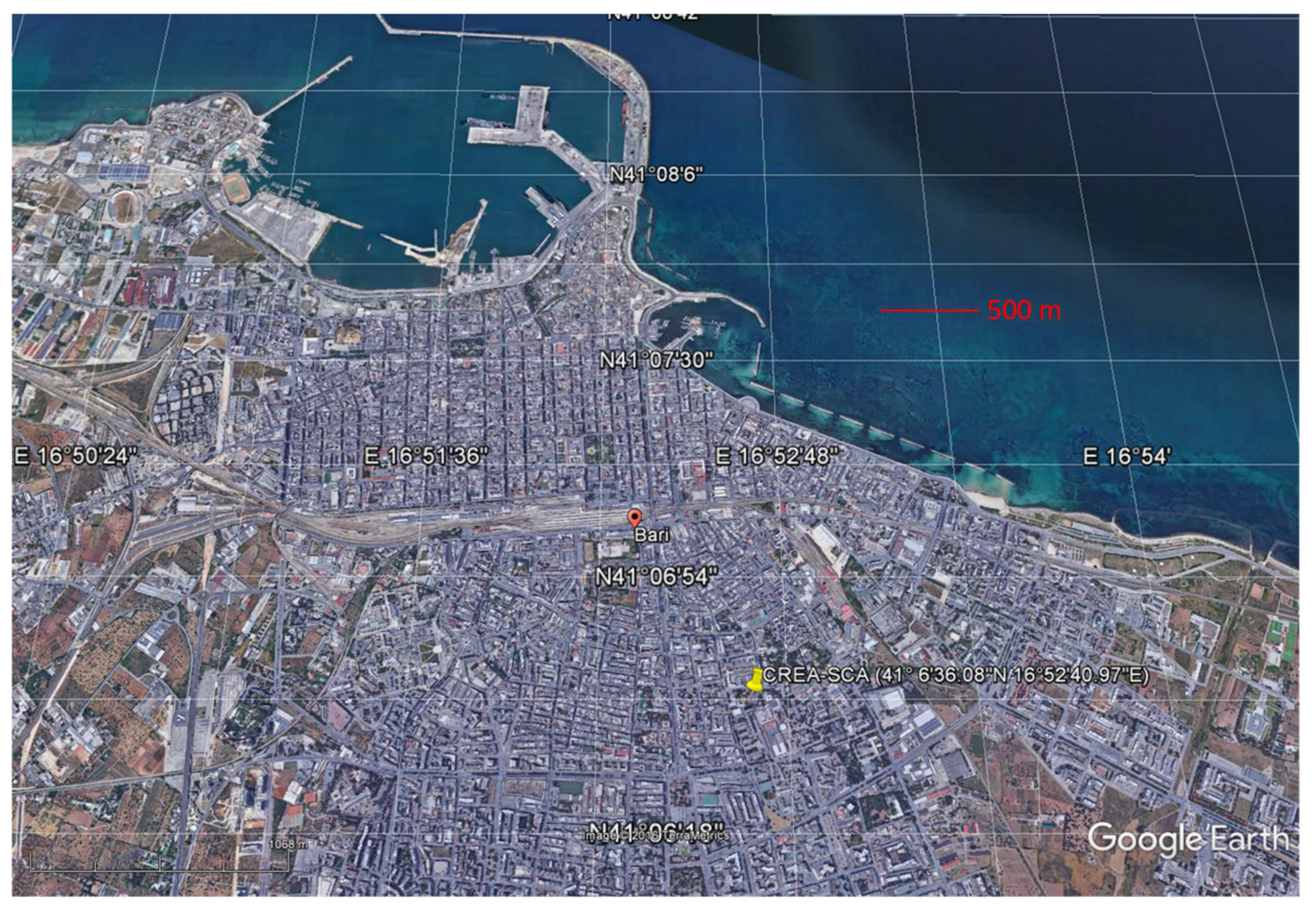
2.1. The Site and the Set Up

The trial was carried out in Bari, a coastal city on the Adriatic Sea of around 320,000 inhabitants on a surface of 117.39 km² located in Southern Italy (Figure 1). The EC tower was set up on the roof of the CREA-AA research institute site, a public historic building (late 19th century), located in a residential area with many public offices, schools, and the university campus. The main types of building structures considering a radius of 500 m from the measuring tower are shown in Figure 2. In the north-eastern sector (I quadrant), a large green surface of large trees is visible (mainly spruce with some cypress and eucalyptus); the south-east sector (II quadrant) hosts the university campus, with high and small buildings, green areas covered by shrubs, small trees, and grass; in the south-western sector (III quadrant), only big roads and civil buildings are present; the remaining north-western sector (IV quadrant) hosts schools and public offices among some private buildings. The EC-tower building is surrounded by a garden with shrubs, grass, and trees of different species (mainly olive, citrus, broadleaves, and conifers) [27].

The experimental campaign started on 7 March 2012 and finished on 17 June 2012, covering a transition period between winter, characterized by domestic heating and intensive vehicle traffic for scholar and public offices activities, and spring, characterized by vehicle traffic and active growth of urban vegetation.

Measured values of CO₂ fluxes are compared to the actual gas consumption of the city. Natural gas used for domestic heating and cooking is usually provided by two pumping stations by Amgas Srl, established in Bari since 2003. Here the values of gas consumption, as provided by the station serving the monitored district, are presented in m³ day⁻¹. The city of Bari did not have any limited traffic zone, therefore no official value of circulating vehicles was available: However, during the scholar activities, the vehicle traffic was obviously most intensive in the area around the monitoring point of this study due the prevalence of public offices (see Figure 2).

The EC equipment did not work between 11 April at 10:30 and 18 April at 8:30, therefore the measurements cover a period of 96 days, from the end of winter up to the end of spring.

The weather in the experimental period followed the seasonal patterns typical of the Bari climate. Daily mean values of air temperature (minimum and maximum), relative humidity, global radiation, and precipitations are shown in Figure 3a, for the period of 1 March–30 June 2012.

Considering that the city developed along the Adriatic Sea (see Figure 1), thus benefiting of the afternoon breeze, the analysis of the predominant wind directions was carried out separately for morning (from 6:00 until 12:00) and afternoon (from 12:00 until 18:00). Figure 3b shows the percentage number of times the wind blew from each 10° sector; in the morning the wind comes from inland (mainly west and north-west), while in the afternoon the wind generally comes from the sea (north and north-east), following the breeze regime until sunset.

The sensors were installed on a 3.5 m mast mounted on a small turret (2 m high, with a floor area of 7 m²) on the roof of the building 12 m above street level, thus the measuring point was positioned at a total height of 17.5 m above street level. The building has the shape of a rough parallelepiped with a surface of 28 × 31 m².

The EC tower system was equipped with a fast-responding open-path infrared gas analyzer for water vapor (H₂O) and CO₂ (IRGA, LI-7500, Li-COR Inc., Lincoln, NE, USA) and a three-dimensional sonic anemometer Gill-R2 (Gill Instruments Ltd., Lymington, UK). The LI-7500 sensor was placed 0.3 m to the side of the anemometer in order to avoid flow disturbances.

The Municipality of Bari imposed by law the switch-off of domestic heating on 31 March 2012; in the first half of June, school holidays began (with complete interruption of lessons and reduction of university activities) in Southern Italy. The trial covers a transition period between intensive and reduced activities of schools and workplaces. The measurement periods and the main events are summarized in

Table 1. Main events during the experimental period.

Date	Event
7 March	Start of CO2 flux measurements
31 March	Household heating official switch off
11–18 April	Failure of equipment
1 June	Beginning of school holidays and reduction of university activities
17 June	End of CO2 flux measurements

.

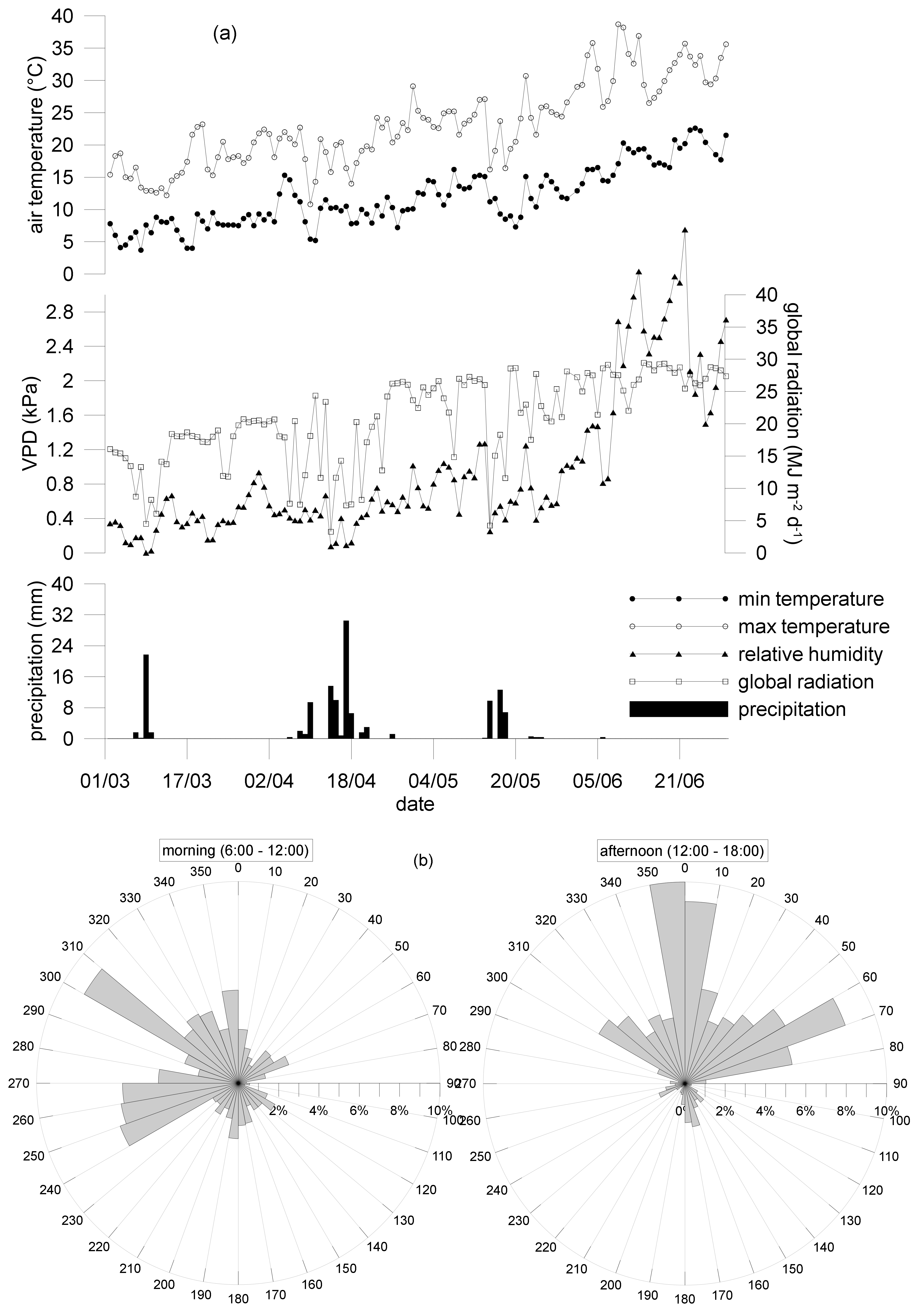
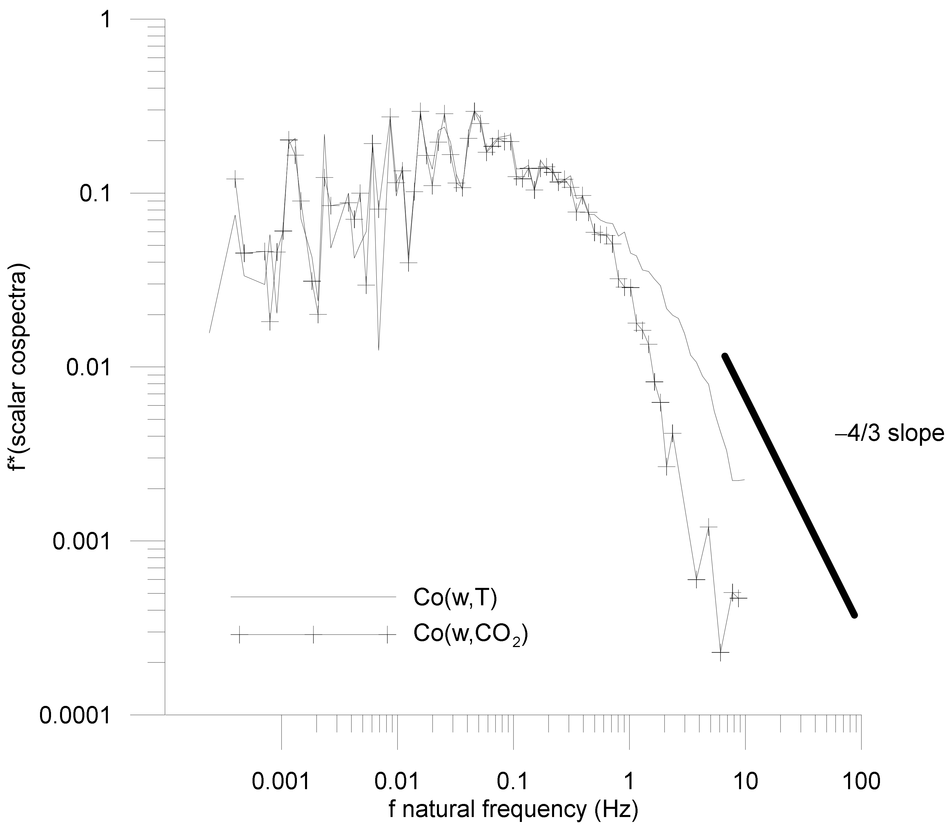
2.2. Measurements and Data Processing

Fluxes of CO₂ were measured by the eddy covariance method [1,28], in which the net flux F in μmol m⁻² s⁻¹, is given by:

$$F=\overline{{\rho }_a}\overline{w\prime \chi \prime }$$

(1)

where ${\rho }_a$ is the air density, $w^{\prime }$ and $\chi \prime$ are the departures from the mean of the vertical wind component and the mean mass of a scalar per unit mass of dry air, respectively.

Following [29], micrometeorological measurements were recorded at 20.8 and 10 Hz, for wind and concentration, respectively, by the EddySoft resident software, and half-hourly fluxes were computed offline using EddyPro^® 4.2 (www.licor.com/eddypro).

The angle-of-attack correction after [30] was applied to compensate flow distortions for the Gill anemometer. The standard WPL terms [31,32] were taken into account to correct for density fluctuations.

Following the suggestion by some authors in the literature [33,34], no friction velocity screening was used. The stationarity and developed turbulence tests of [35] were calculated for all fluxes, but in this case we did not follow the standard procedure to discard the fluxes flagged as “2” (as done normally in non-urban context), since these classifications could lead to considerable data loss for urban areas [34,36].

Spectral analysis was used to verify the quality of the acquisition frequency applied on site, and averaging time interval used for the fluxes. An example of averaged and normalized scalar cospectra of sensible heat and CO₂ is reported in Figure 4 for the runs from 11:00 to 15:00 during a clear day. Both cospectra agreed well with the theoretical −4/3 slopes in the inertial subrange. The low damping in the CO₂ fluxes was corrected, at high and low frequencies, applying the method proposed by [37].

In order to verify Taylor’s turbulence frozen hypothesis, the turbulence intensity is determined by standard deviations of wind vector divided by horizontal wind velocity U [38] as:

$$I_i=\frac{{\sigma }_i}{U} \left(i=u, v, w\right)$$

(2)

I_i < 0.5 is required for Taylor’s hypothesis to be verified [38]. Mean values for the different wind vector components under neutral stability found at this site are I_u = 0.38, I_v = 0.30, I_w = 0.14; these are in agreement with urban values reported by other authors [20,39,40].

The flux random uncertainty due to sampling errors was calculated according to [41], giving overall estimates of 7.4 ± 7 W m⁻² for sensible heat and 2.3 ± 7.3 μmol m⁻² s⁻¹ for CO₂ fluxes, respectively; other considerations on the random errors are reported in Appendix A. The steady state classification according to [35] showed that the suspicious fluxes (class 2) amounted to 2% and 10% for sensible heat flux (H) and CO₂, respectively, for daylight values, increasing to 10% and 25%, respectively, for night time, when often stable conditions prevail.

One-way ANOVA was applied to daily mean CO₂ fluxes, after testing normality (Kolmogorov–Smirnov test) and homogeneity of variance (Bartlett test), for the period before and after heating switching (31 March). This statistical analysis was carried out using the free software environment R (R Development Core Team, 2014. http://cran.r-project.org/).

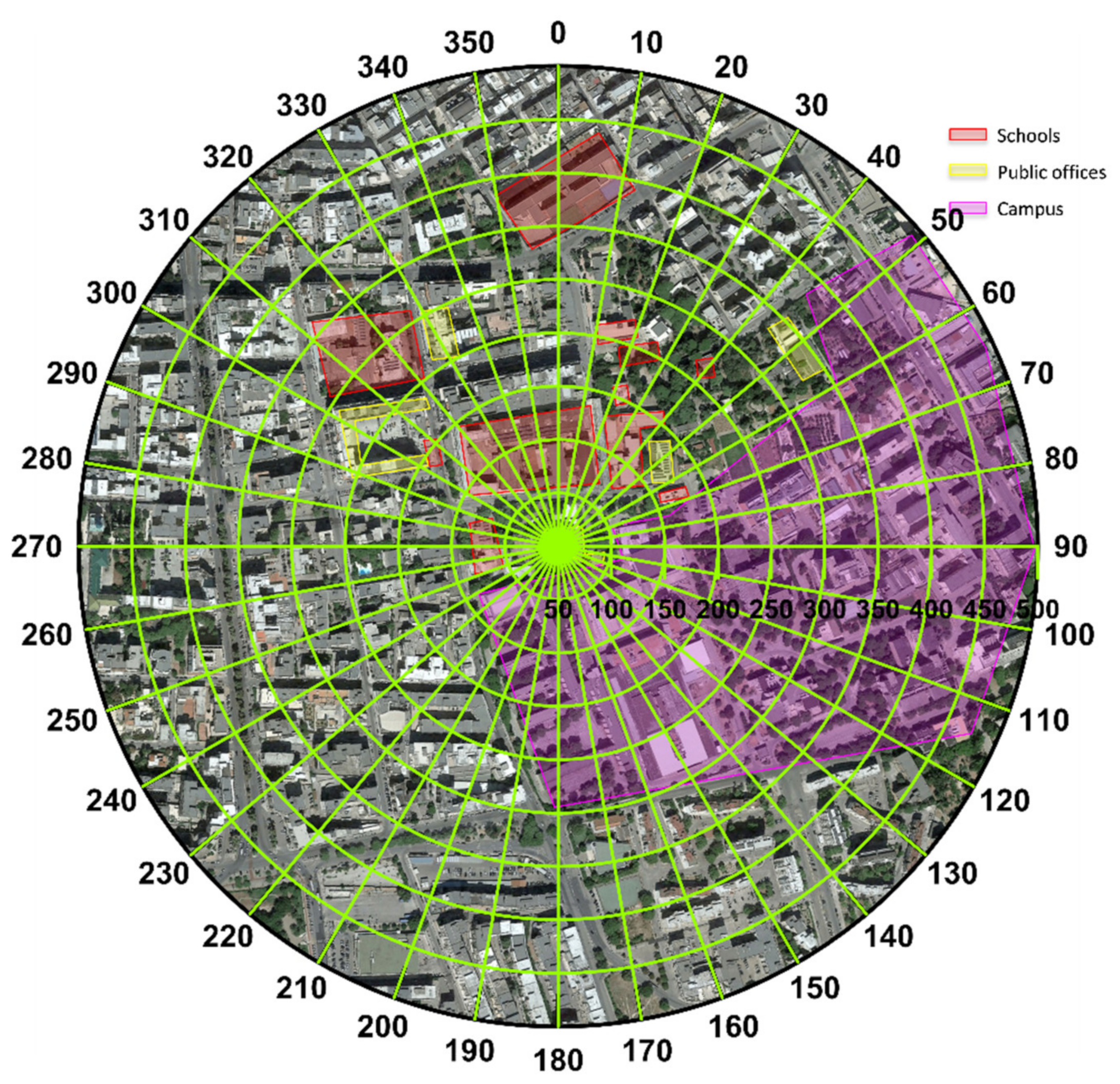
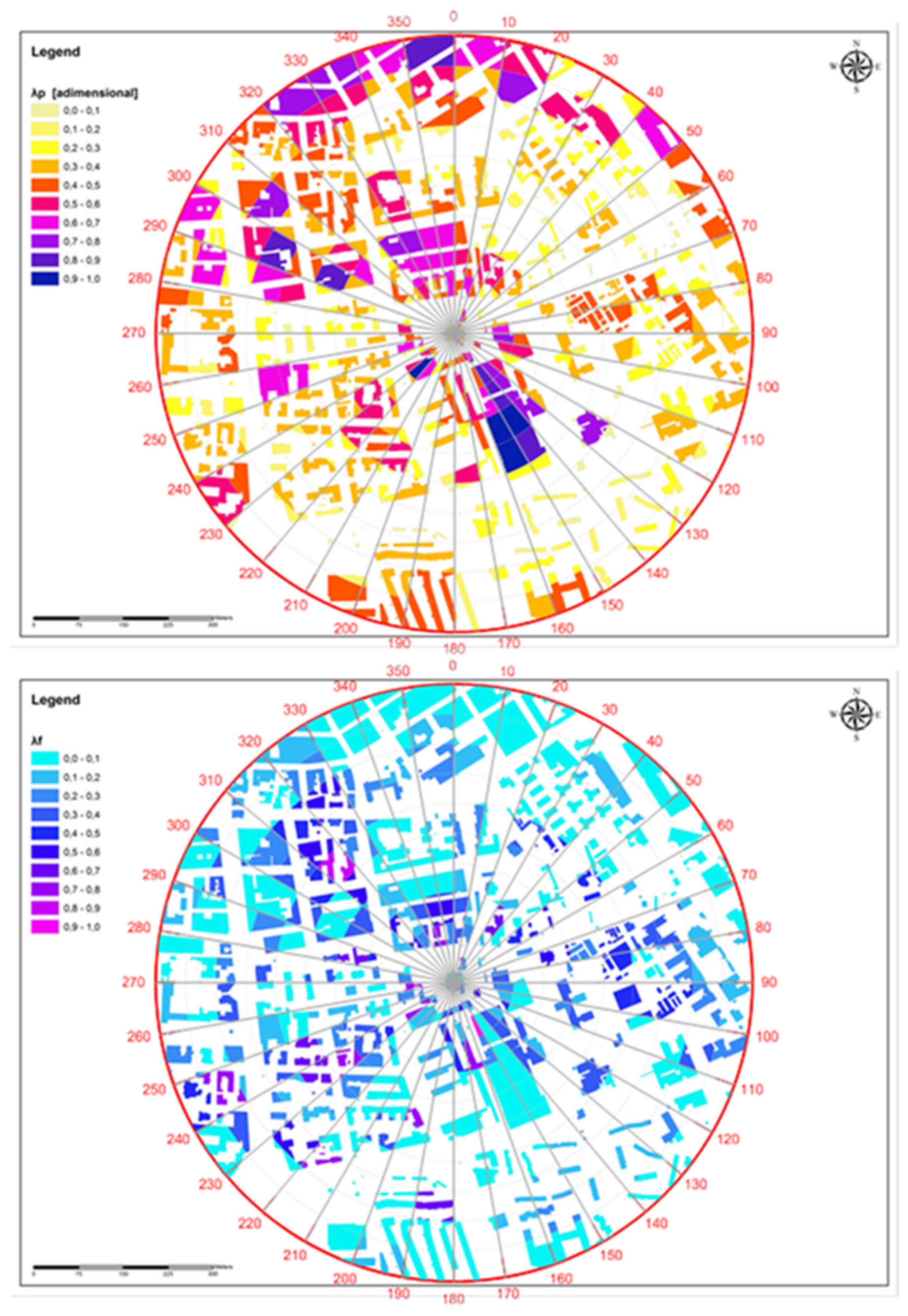
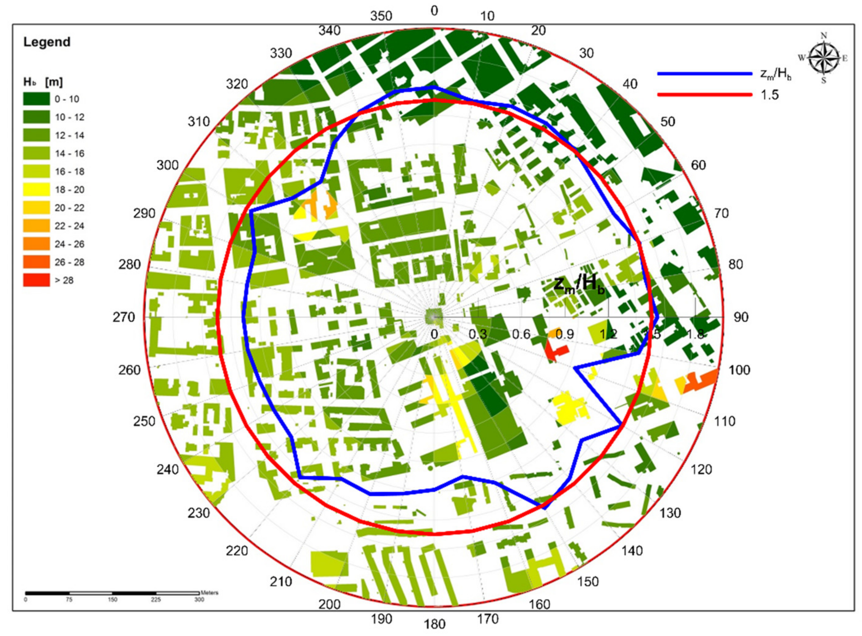
2.3. Morphological Characteristics and CO₂ Source Areas of the Site

The footprint notion is often used to describe the source area of turbulent scalar fluxes [42]. In this study, the source areas of CO₂ fluxes, in terms of distance from the EC measurement point, were calculated run by run, following the procedure from Kotthaus and Grimmond [25]. The footprint (x, in m) was determined as a function of wind speed and direction, roughness length (z₀, in m), and displacement plane height (d, in m) at the site. In this case, d and z₀ were determined as reported by MacDonald et al. [43], using the morphological parameters (building height H_b in m, frontal area fraction λ_f, and plan area fraction λ_p) relative to the cells individuated inside the area of 500 m radius centered in the EC tower, for every 50 m and 10° interval sectors (324 cells, see the scheme of cells in Figure 2). In particular:

$${\lambda }_p=\frac{A_p}{A_d}$$

(3)

$${\lambda }_f=\frac{A_f}{A_d}$$

(4)

with A_p, A_d, and A_f being the plan area in m² occupied by buildings, the area of the cell, and the frontal area of buildings oriented toward the EC measurement point, respectively. A_f is calculated as indicated in [44], as it is a function of orientation, θ, of the frontal area of the buildings. The projection of the building surface along the wind direction is given by the dot product between this vector and a horizontal unit vector in the direction θ. The detailed procedure to calculate the source areas is presented in Appendix B.

3. Results and Discussion

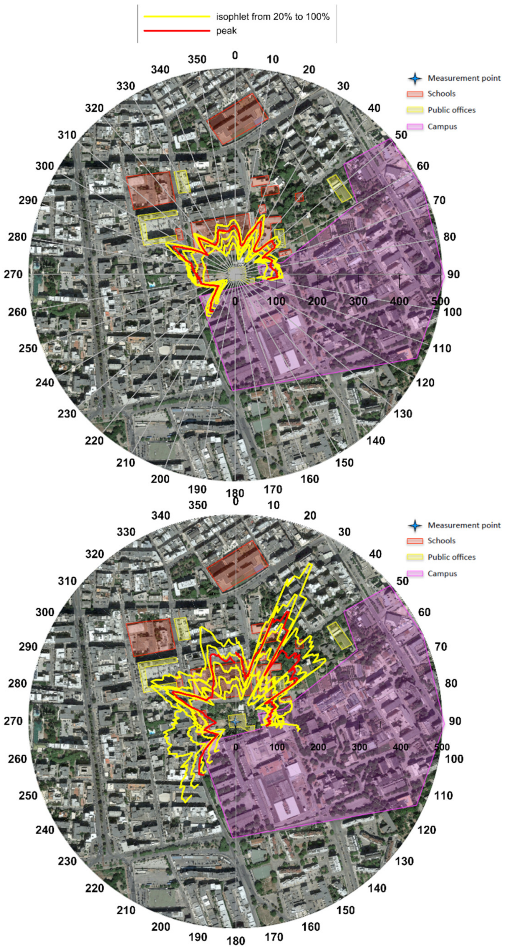
3.1. Source Area

The level of patchiness of the studied area can be deduced by the values of λ_f and λ_p, illustrated in Figure 5. In fact, λ_p has the lowest value in the sectors between 60° and 80°, corresponding to the areas with fewer buildings and large vegetation cover, while the highest values are in the north-west and south-east sectors, hosting many civil buildings and the university campus, respectively (see Figure 2). λ_f assumes the lowest value always in the direction with large vegetation area at north-east, but also at south south-east, where the university campus hosts both high and low scattered buildings. Figure 6 shows the distribution of the mean building heights for each cell and the mean values of the ratio between the measurement height (z_m) and H_b of all cells in each sector of 10°. Moreover, in Figure 6, the ratio between z_m and the H_b found by Kljun et al. [45], above which the divergence of fluxes vanishes, is highlighted (equal to 1.5). It is clear that the requirement of 1.5 for having acceptable measurements is completely satisfied in the sector 330–100°, while a lower value around 1.3–1.4 was accepted for the sector 210–330°. The ratio between z_m and the H_b was considered too low.

The source area of EC fluxes is strongly affected by the atmospheric stratification [42]. Following [23], the chosen atmospheric stability parameter is ζ = z′/L, with L Obukhov length and z′ effective height z′ = z_m − d (z_m and d are measurement and displacement height, respectively). The used stability classification is ζ < −0.1, −0.1 ≤ ζ ≤ 0.1, and ζ > 0.1 for unstable, near neutral, and stable conditions, respectively; the number of runs in stable conditions is negligible (3%) for all sectors, and not further considered in the flux analysis, while the number of runs in neutral and unstable conditions represent 50.5% and 46.5% of the total, respectively. The percentage of runs with the wind coming from the sectors between 100° and 210° (not considered in the analysis of CO₂ fluxes) is 17% (9% in neutral and 8% in unstable conditions). The unstable conditions occurred during daytime on 65% of the total cases, while neutral conditions in 58% of total cases during the night. Stable conditions were found exclusively during the night.

The results of this calculation are reported in Figure 7 for neutral and unstable conditions: The isopleths represent the 20, 40, 60, 80, 100% of the source areas, calculated by aggregating all data, showing a larger surface area under neutral conditions than unstable conditions. The footprint calculation relative to the sector between 100° and 210° failed to return feasible results, i.e., no footprint value met the conditions required by the Kormann and Meixner’s model, confirming that when the wind comes from that sector, the measurement point is inside the roughness sublayer and well below the blending height, jeopardizing the hypotheses of the method. For this reason, the sector was excluded from the flux analysis.

In unstable conditions, the source areas of CO₂ fluxes contained public facilities buildings, the vegetated area surrounding the measuring tower, a single-carriage road which passes through the schools and public offices, and a very busy road east of the measuring point which links the outskirts to the city center. In neutral conditions, the source area was extended to private residence buildings, roads, and the large vegetation area in the north-east direction.

In Figure 7, the footprint peak is also reported, as a red line; it was always between 50 and 150 m away from the roof of the building with the EC tower, in both unstable and neutral situations.

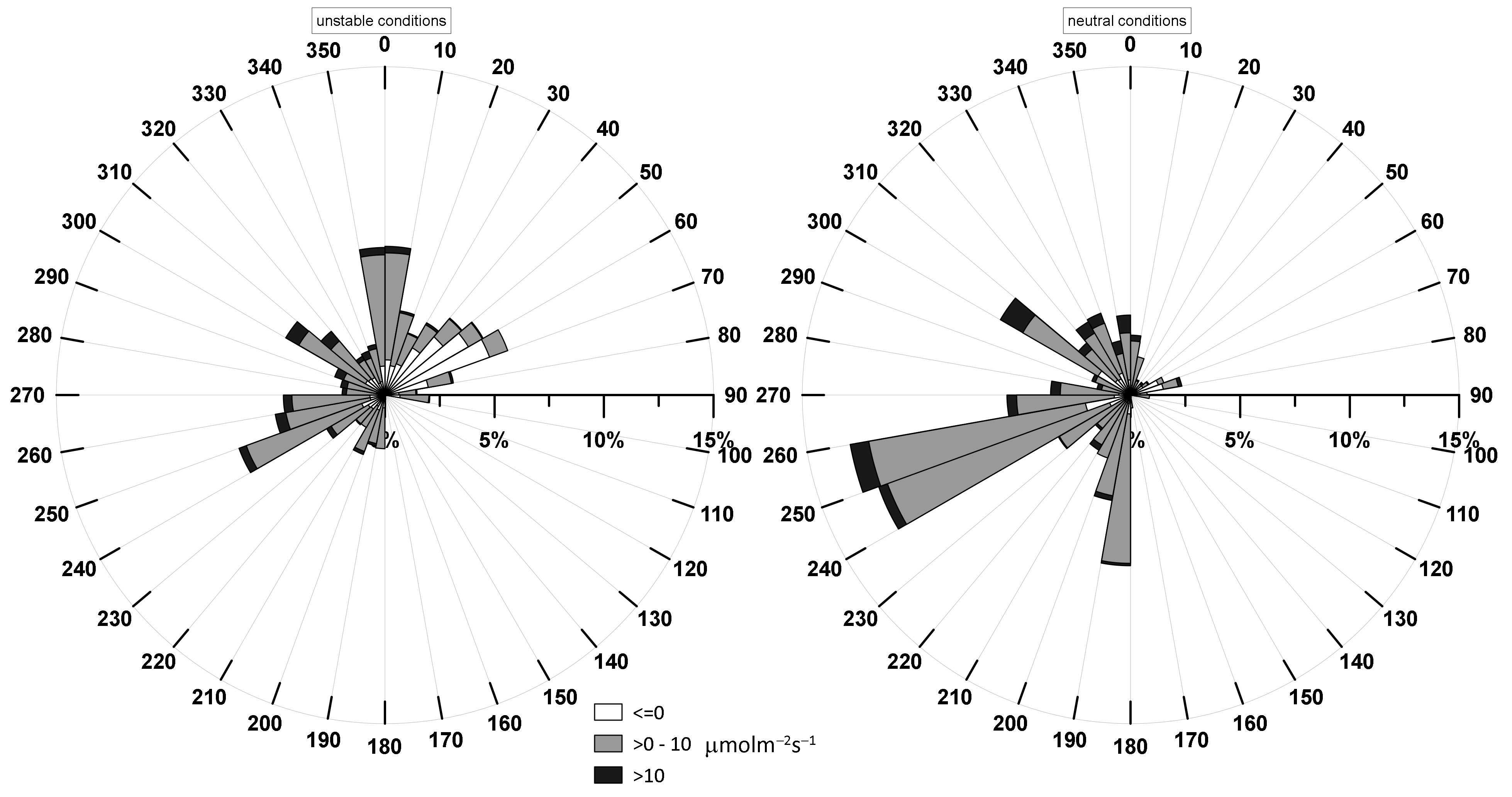
3.2. CO₂ Fluxes and Anthropogenic Activities

3.2.1. Landscape

Firstly, the relationship between wind direction and CO₂ fluxes around the measurement tower is analyzed. In Figure 8, the measured CO₂ fluxes (μmol m⁻² s⁻¹) are shown for each 10° sector, in unstable (left) and neutral (right) conditions, for the whole experimental period; the half-hourly fluxes are subdivided in three classes: ≤0 μmol m⁻² s⁻¹, i.e., CO₂ uptake by the ecosystem, 0–10 μmol m⁻² s⁻¹, i.e., moderate emissions, and ≥10 μmol m⁻² s⁻¹, i.e., high emissions. For unstable conditions, the majority of CO₂ emissions came from the big busy streets and schools between south-west and north. The north-east sector, where a large green surface is located, with big trees just close to the measurement point above the historical building, was never a source of CO₂ in unstable conditions. In this case, the presence of trees and the vegetation, with their diurnal photosynthetic activity, probably contributes with a CO₂ uptake, mitigating the otherwise emissive character of the urban area, similarly to the mitigation effect of vegetation on CO₂ emissions observed by Grimmond et al. [20] on Marseille. In fact, a one-way ANOVA for comparing, at hourly scale, (1) the mean of CO₂ fluxes when the wind direction was inside the I quadrant (north-east) and (2) the mean of fluxes when the wind direction was in the other sectors (see Figure 2) showed a highly significant difference (p < 0.00001), with lower values in the first case, i.e., when the wind came from the area containing large vegetated surfaces (

Table 2. Comparison between mean hourly CO₂ fluxes, as measured during the whole experimental period, in function of wind direction (one way—ANOVA).

Wind Direction	Runs (n)	Mean CO2 Fluxes (μmol m−2 s−1)	Standard Deviation (μmol m−2 s−1)	Mean Random Error (μmol m−2 s−1)
I quadrant (north-east)	918	−0.25	21.7	1.35
others	2416	+4.00	117.8	2.43

). In Table 2, the mean random error is also reported for both cases.

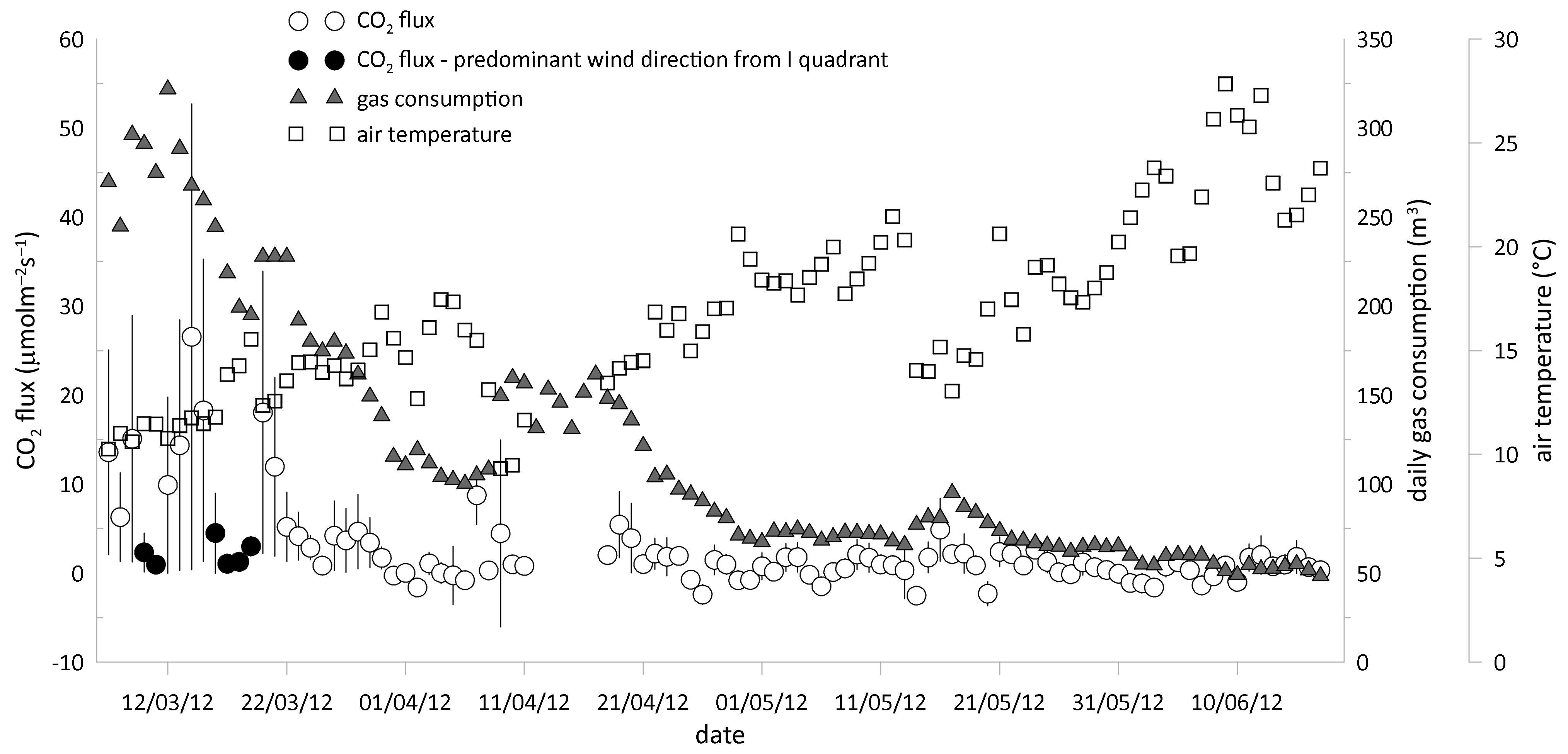
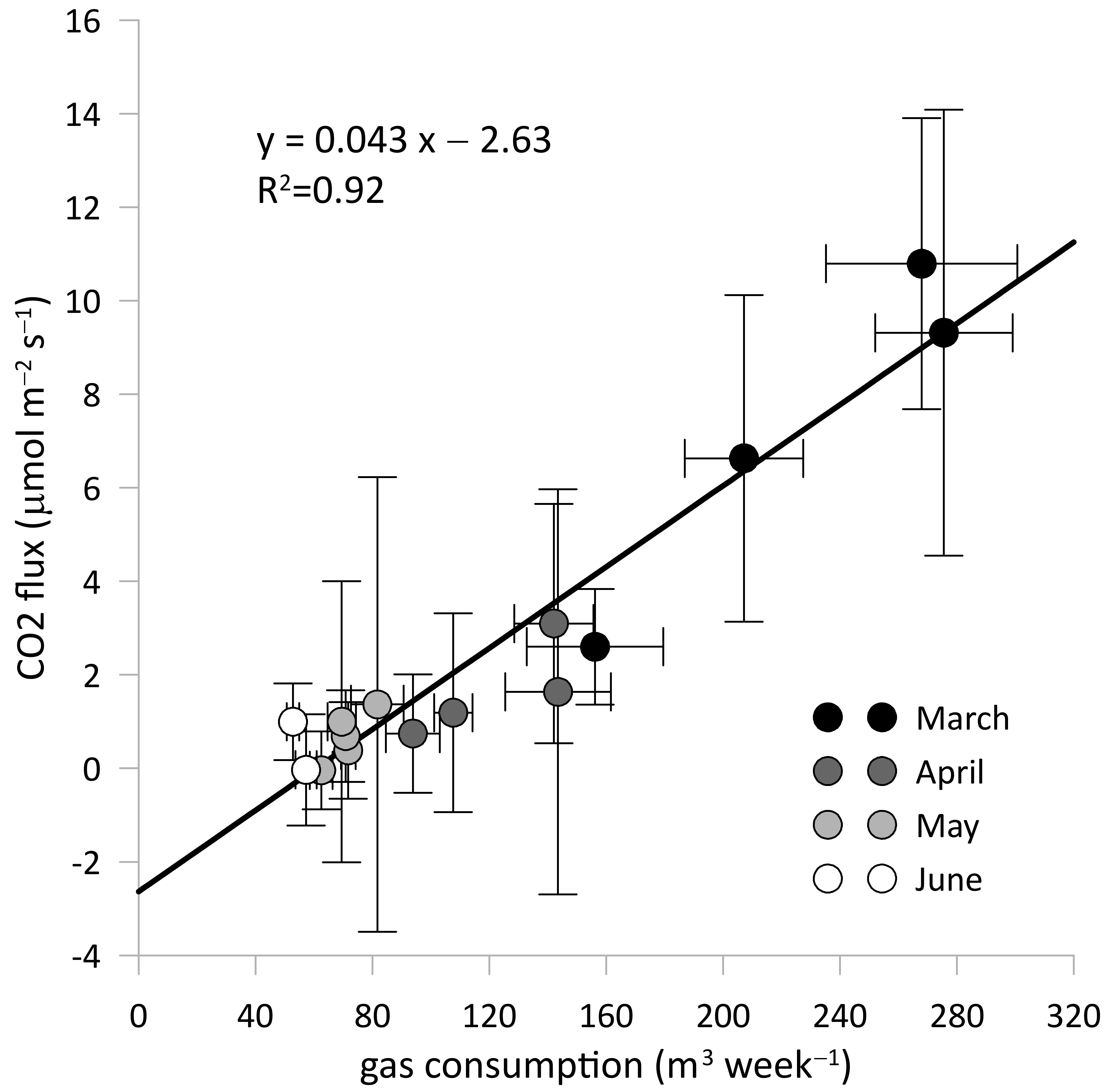
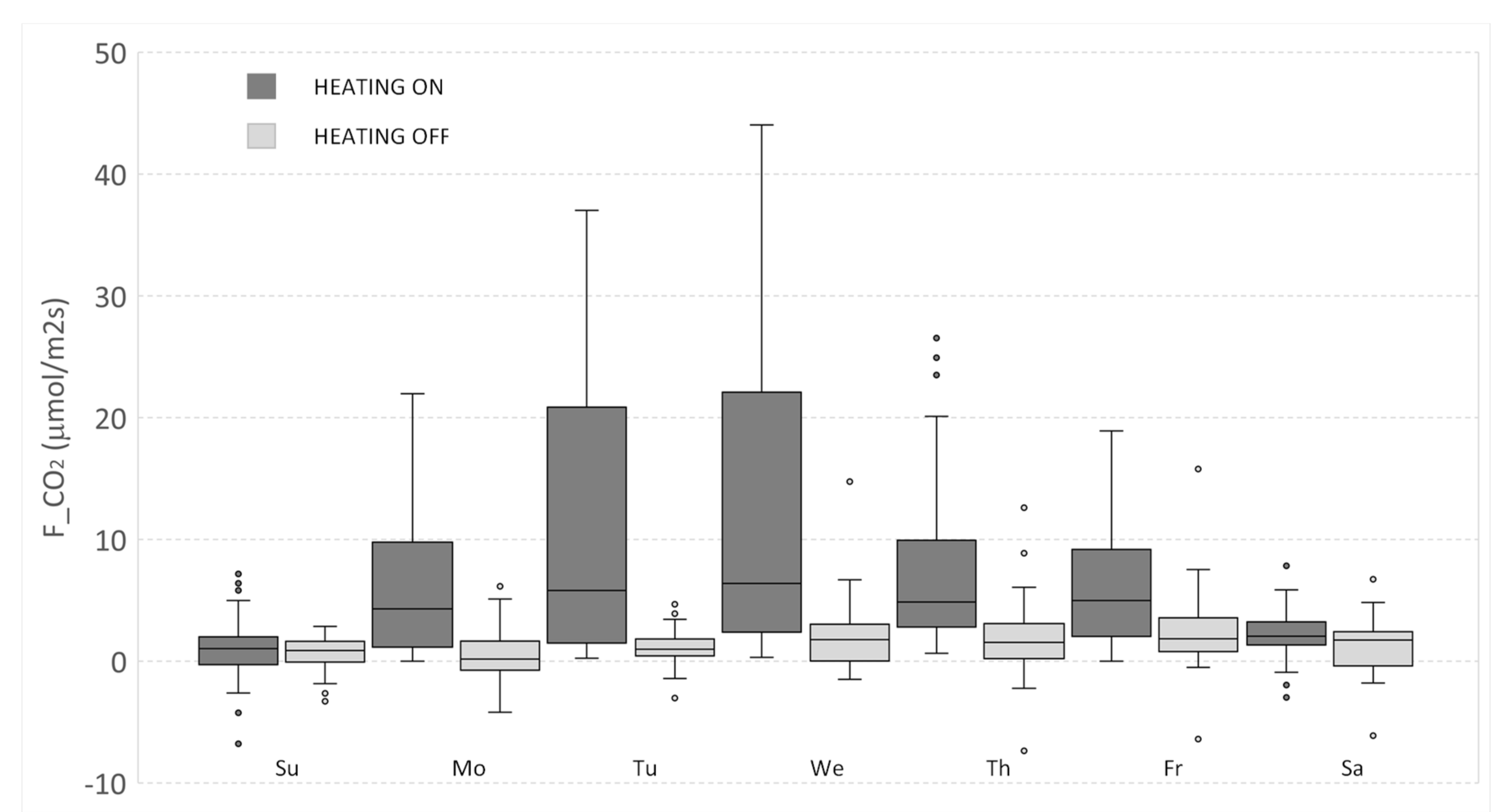
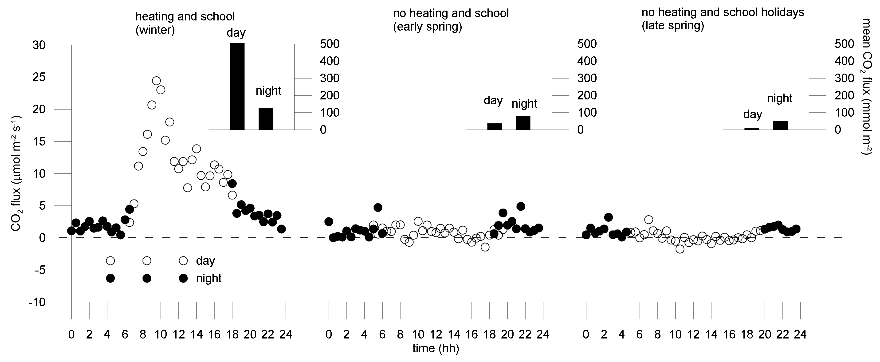
3.2.2. Domestic Heating

The dynamics of CO₂ flux, the gas consumption, and the air temperature as average at daily scale are shown in Figure 9.

From the figure, it is clear that the CO₂ fluxes are highest in the month of March, corresponding to the highest gas consumption values. This is in accordance with the consideration that in Bari, the domestic heating is switched off by law on 31 March. The highest CO₂ fluxes are, moreover, in correspondence with lowest air temperature values. Furthermore, from Figure 9 it can also be noticed that the emissions of CO₂ are partially compensated by the photosynthetic activity of vegetated surfaces, when the predominant wind came from the I quadrant (north-east, black circles).

The relationship between CO₂ fluxes and gas consumption in the experimental period is evaluated considering the average at weekly scale in Figure 10. A clear linear dependence is highlighted with a high value of R². The values are largely spread (high standard deviations) during the months presenting highest values of CO₂ flux (March and April).

Table 3. F values and P-values of the one-way ANOVA applied to mean daily CO₂ fluxes for each day of the week, before and after the heating switching off (Significant codes: *** p < 0).

Day of the Week	F-Value	p-Value
Sunday	0.792	0.376
Monday	40.46	7.21 × 10−9 ***
Tuesday	37.43	2.28 × 10−8 ***
Wednesday	28.85	5.97 × 10−7 ***
Thursday	25.67	2.04 × 10−6 ***
Friday	22.75	6.74 × 10−6 ***
Saturday	3.863	0.0523

shows F values and P-values of a one-way ANOVA applied to mean daily CO₂ fluxes for each day of the week before and after the heating switching off. Figure 11 shows a box plot of CO₂ fluxes representative for each day of the week for the two contrasting periods (heating ON and heating OFF).

In particular, the differences between the two periods are highly significant for the workdays of the week, between Monday and Friday, clearly suggesting the relationship with the highest gas consumption required by working and scholar activities, and their interruption during the weekend.

From these results, it is evident that the investigated area is a strong source of CO₂ during winter, with the heating on, especially during weekdays from Monday to Friday, with peak values around the center of the week (Wednesdays). During the winter weekends, emissions of CO₂ are reduced because in the surrounding area the majority of buildings are public places as schools, the university, and offices, normally closed during weekends. After March, with the heating switched off, the daily course of CO₂ fluxes does not present a clear pattern within the week. Further investigations are necessary to better describe the possible turbulence pumping effect in the central part of the week.

3.2.3. Local Traffic

Without a measured number of vehicles circulating in the area due to the absence of a monitoring of the municipality, the behavior of CO₂ fluxes can be only qualitatively linked to the local traffic, which appears more relevant when the heating component is off. The chosen period to investigate the relationship between local traffic and CO₂ emissions in the experimental area was identified from May until the end of the trial in June, including the closure of the schools and university for the summer holidays (after 1 June), and the consequent decrease of traffic around the EC tower in the actual source area (see Figure 7). In general, the CO₂ mean fluxes during workdays (Monday to Friday) are slightly higher during the school period. In fact, calculating the cumulative sum of all CO₂ fluxes during this period, the values are +1210 and +783 mmol m⁻² period⁻¹ for the workdays before and after the school holiday, respectively, with a reduction of 35% of the total CO₂ emissions during holiday periods. During weekends, the CO₂ fluxes are always positive or slightly negative during the day, because of the presence of quite large green surfaces with big trees, which during the spring have a strong photosynthetic activity.

Finally, the patterns of the CO₂ fluxes during the day at an hourly scale (averaged over the different periods) show specific peculiarities for the three targeted periods: Heating and school, no heating and school, no heating and school holidays. The results illustrated in Figure 12, in fact, clearly show that in the first period, when the heating is working, the emissions of CO₂ are always positive both during daytime and night time, with cumulated mean daily values of 506 mmol m⁻² d⁻¹ and 127 mmol m⁻² d⁻¹, respectively (see the bar panels at the right of each panel in Figure 12). During the second period, when the heating is switched off, the CO₂ fluxes greatly decrease, being almost always positive during the day, and with more similar values for day and night (37 and 80 mmol m⁻² d⁻¹, respectively). During the third period, with reduced traffic for the school holidays and no heating, the emissions are further reduced, being 8 and 50 mmol m⁻² d⁻¹ for day and night, respectively. Furthermore, during the day, the CO₂ fluxes are slightly but consistently negative, showing a clear uptake of CO₂ by the vegetation around the experimental area. In this case, the photosynthetic activity seems to play an important role during the day by mitigating the CO₂ emissions and should be studied in more detail.

4. Conclusions

This study reports a morphological analysis of the source area and a footprint analysis within an urban context, using EC-CO₂ fluxes measured in a district of a coastal city in southern Italy, between the end of winter and the end of spring. The eddy covariance measurements were carried out on the roof of a laboratory research site, surrounded by green surfaces and trees. The ratios of measurement-height/buildings-height of the source area were in the range 1.3–1.5. However, despite the fact that the measurement point of EC fluxes in this study was not placed at an ideal height, the source area was determined in great detail run by run, showing different representativeness of source areas according to stability conditions. Under unstable conditions, the source area includes only public buildings (schools, offices, research centers, the university campus) and a single road connecting all structures. In neutral conditions, the source area is extended to private buildings and relatively busy roads. A big green area, north-east of the measurement site, also markedly influences the CO₂ sink/source characteristics. A sector of 90° in the south-east direction is excluded from the analysis due to the proximity of big buildings which do not meet the requirements for the correct calculation of the source area.

The effects of heating, vehicle traffic, and vegetation on CO₂ fluxes supported the source area analysis. In particular, the results showed that the experimental area is almost always a source of CO₂. However, the presence of big trees and other vegetative surfaces seems to mitigate the CO₂ emissions when the growing season starts. When the domestic heating was on, the area emitted large amounts of CO₂, especially during workdays, with a reduction of 82% when the heating was switched off. A further reduction of 50% was measured at the closing of the schools for summer holidays and consequent traffic reduction. These insights could be well used to regulate the heating at least in public structures (to shorten and better schedule the functioning time), and to understand a way to reduce the impact of the traffic on human health.

Further research is evidently desirable for linking the photosynthetic activity of vegetation and the evapotranspiration to the CO₂ sink/source of this particular urban area to mitigate the impacts of carbon dioxide and other pollutants.

Finally, even if the investigated area was too restricted to allow a generalization of the results to the whole city, it is evident that the CO₂ sink/source character of a well delimited area can be anyway related with specific anthropogenic and vegetation activities, by implementing a parameterization of the footprint for each individual run, which draws a clear picture of the morphological characteristics for each flux event.

References

1. Aubinet, M.; Vesala, T.; Papale, D. Eddy Covariance—A Practical Guide to Measurement and Data Analysis; Springer: Dordrecht, The Netherlands; Berlin/Heidelberg, Germany; London, UK; New York, NY, USA, 2012; p. 307. [Google Scholar] [CrossRef]
2. Ramamurthy, P.; Pardyjak, E.R. Toward understanding the behavior of carbon dioxide and surface energy fluxes in the urbanized semi-arid Salt Lake Valley, Utah, USA. Atmos. Environ. 2011, 45, 73–84. [Google Scholar] [CrossRef]
3. Liu, H.Z.; Feng, J.W.; Järvi, L.; Vesala, T. Four-year (2006–2009) eddy covariance measurements of CO2 flux over an urban area in Beijing. Atmos. Chem. Phys. Discuss 2012, 12, 7881–7892. [Google Scholar] [CrossRef] [Green Version]
4. Velasco, E.; Pressley, S.; Allwine, E.; Westberg, H.; Lamb, B. Measurements of CO fluxes from the Mexico City urban landscape. Atmos. Environ. 2005, 39, 7433–7446. [Google Scholar] [CrossRef]
5. Coutts, A.; Beringer, J.; Tapper, N.J. Characteristics influencing the variability of urban CO2 fluxes in Melbourne, Australia. Atmos. Environ. 2007, 41, 51–62. [Google Scholar] [CrossRef]
6. Nemitz, E.; Hargreaves, K.J.; McDonald, A.G.; Dorsey, J.; Fowler, D. Micrometeorological Measurements of the Urban Heat Budget and CO2Emissions on a City Scale. Environ. Sci. Technol. 2002, 36, 3139–3146. [Google Scholar] [CrossRef] [PubMed]
7. Grimmond, S.; King, T.; Cropley, F.; Nowak, D.; Souch, C. Local-scale fluxes of carbon dioxide in urban environments: Methodological challenges and results from Chicago. Environ. Pollut. 2002, 116, S243–S254. [Google Scholar] [CrossRef]
8. Moriwaki, R.; Kanda, M. Seasonal and Diurnal Fluxes of Radiation, Heat, Water Vapor, and Carbon Dioxide over a Suburban Area. J. Appl. Meteorol. 2004, 43, 1700–1710. [Google Scholar] [CrossRef]
9. Vesala, T.; Järvi, L.; Launiainen, S.; Sogachev, A.; Rannik, Ü.; Mammarella, I.; Siivola, E.; Keronen, P.; Rinne, J.; Riikonen, A.; et al. Surface–atmosphere interactions over complex urban terrain in Helsinki, Finland. Tellus B Chem. Phys. Meteorol. 2008, 60, 188–199. [Google Scholar] [CrossRef] [Green Version]
10. Velasco, E.; Pressley, S.; Grivicke, R.; Allwine, E.; Coons, T.; Foster, W.; Jobson, B.T.; Westberg, H.; Ramos, R.; Hernandez, F.; et al. Eddy covariance flux measurements of pollutant gases in urban Mexico City. Atmos. Chem. Phys. Discuss 2009, 9, 7325–7342. [Google Scholar] [CrossRef] [Green Version]
11. Helfter, C.; Famulari, D.; Phillips, G.J.; Barlow, J.F.; Wood, C.R.; Grimmond, S.B.; Nemitz, E. Controls of carbon dioxide con-centrations and fluxes above central London. Atmos. Chem. Phys. 2011, 11, 1913–1928. [Google Scholar] [CrossRef] [Green Version]
12. Pawlak, W.; Fortuniak, K.; Siedlecki, M. Carbon dioxide flux in the centre of Łódź, Poland—analysis of a 2-year eddy covariance measurement data set. Int. J. Climat. 2011, 31, 232–243. [Google Scholar] [CrossRef]
13. Song, T.; Wang, Y. Carbon dioxide fluxes from an urban area in Beijing. Atmos. Res. 2012, 106, 139–149. [Google Scholar] [CrossRef]
14. Lietzke, B.; Vogt, R.; Feigenwinter, C.; Parlow, E. On the controlling factors for the variability of carbon dioxide flux in a heterogeneous urban environment. Int. J. Clim. 2015, 35, 3921–3941. [Google Scholar] [CrossRef]
15. Giorgi, F.; Lionello, P. Climate change projections for the Mediterranean region. Glob. Planet. Chang. 2008, 63, 90–104. [Google Scholar] [CrossRef]
16. Espadafor, M.; Lorite, I.J.; Gavilán, P.; Berengena, J. An analysis of the tendency of reference evapotranspiration estimates and other climate variables during the last 45 years in Southern Spain. Agric. Water Manag. 2011, 98, 1045–1061. [Google Scholar] [CrossRef]
17. Matese, A.; Gioli, B.; Vaccari, F.; Zaldei, A.; Miglietta, F. Carbon Dioxide Emissions of the City Center of Firenze, Italy: Measurement, Evaluation, and Source Partitioning. J. Appl. Meteorol. Clim. 2009, 48, 1940–1947. [Google Scholar] [CrossRef]
18. Gratani, L.; Varone, L. Daily and seasonal variation of CO in the city of Rome in relationship with the traffic volume. Atmos. Environ. 2005, 39, 2619–2624. [Google Scholar] [CrossRef]
19. Contini, D.; Donateo, A.; Elefante, C.; Grasso, F. Analysis of particles and carbon dioxide concentrations and fluxes in an urban area: Correlation with traffic rate and local micrometeorology. Atmos. Environ. 2012, 46, 25–35. [Google Scholar] [CrossRef]
20. Grimmond, C.S.B.; Salmond, J.A.; Oke, T.R.; Offerle, B.; Lemonsu, A. Flux and turbulence measurements at a densely buil-up site in Marseille, heat, mass (water and carbon dioxide) and momentum. J. Geoph. Res. 2004, 109, D24101. [Google Scholar] [CrossRef]
21. Kotthaus, S.; Grimmond, C. Energy exchange in a dense urban environment—Part II: Impact of spatial heterogeneity of the surface. Urban Clim. 2014, 10, 281–307. [Google Scholar] [CrossRef] [Green Version]
22. Claussen, M. Estimation of areally-averaged surface fluxes. Boundary-Layer Meteorol. 1991, 54, 387–410. [Google Scholar] [CrossRef]
23. Kotthaus, S.; Grimmond, C.S.B. Identification of Micro-scale Anthropogenic CO2, heat and moisture sources—Processing eddy covariance fluxes for a dense urban environment. Atmos. Environ. 2012, 57, 301–316. [Google Scholar] [CrossRef]
24. Peters, E.B.; Hiller, R.V.; McFadden, J.P. Seasonal contributions of vegetation types to suburban evapotranspiration. J. Geophys. Res. Space Phys. 2011, 116, 01003. [Google Scholar] [CrossRef]
25. Kotthaus, S.; Grimmond, C.S.B. Energy exchange in a dense urban environment—Part I: Temporal variability of long-term observations in central London. Urb. Clim. 2014, 10, 261–280. [Google Scholar] [CrossRef] [Green Version]
26. Rahman, M.A.; Moser, A.; Rötzer, T.; Pauleit, S. Microclimatic differences and their influence on transpirational cooling of Tilia cordata in two contrasting street canyons in Munich, Germany. Agric. For. Meteorol. 2017, 232, 443–456. [Google Scholar] [CrossRef]
27. Rana, G.; De Lorenzi, F.; Mazza, G.; Martinelli, N.; Muschitiello, C.; Ferrara, R.M. Tree transpiration in a multi-species Mediterranean garden. Agric. For. Meteorol. 2020, 280, 107767. [Google Scholar] [CrossRef]
28. Lee, X.; Massman, W.; Law, B.E. Handbook of Micrometeorology: A Guide for Surface Flux Measurement and Analysis; Kluwer Academic Publishers: Dordrecht, The Netherlands, 2004. [Google Scholar]
29. Kolle, O.; Rebmann, C. Eddysoft: Documentatation of a Software Package to Acquire and Process Edy Covariance Data; Max Planck Institute for Biochemistry: Jena, Germany, 2007. [Google Scholar]
30. Wilczak, J.M.; Oncley, S.P.; Stage, S.A. Sonic Anemometer Tilt Correction Algorithms. Bound. Layer Meteorol. 2001, 99, 127–150. [Google Scholar] [CrossRef]
31. Nakai, T.; Van Der Molen, M.; Gash, J.; Kodama, Y. Correction of sonic anemometer angle of attack errors. Agric. For. Meteorol. 2006, 136, 19–30. [Google Scholar] [CrossRef] [Green Version]
32. Webb, E.K.; Pearman, G.; Leuning, R. Correction of flux measurements for density effects due to heat and water vapour transfer. Quart. J. Roy. Meteor. Soc. 1980, 106, 85–100. [Google Scholar] [CrossRef]
33. Bargeron, O.; Strachan, I. CO2 sources and sinks in urban and suburban areas in a northern mid-altitude city. Atosp. Environ. 2011, 45, 1564–1573. [Google Scholar]
34. Ward, H.C.; Evans, J.G.; Grimmond, S. Multi-season eddy covariance observations of energy, water and carbon fluxes over a suburban area in Swindon, UK. Atmos. Chem. Phys. Discuss 2013, 13, 4645–4666. [Google Scholar] [CrossRef] [Green Version]
35. Foken, T.; Wichura, B. Tools for quality assessment of surface-based flux measurements. Agric. For. Meteorol. 1996, 78, 83–105. [Google Scholar] [CrossRef]
36. Fortuniak, K.; Pawlak, W.; Siedlecki, M. Integral Turbulence Statistics Over a Central European City Centre. Bound. Layer Meteorol. 2012, 146, 257–276. [Google Scholar] [CrossRef]
37. Moncrieff, J.; Massheder, J.; De Bruin, H.; Elbers, J.; Friborg, T.; Heusinkveld, B.; Kabat, P.; Scott, S.; Soegaard, H.; Verhoef, A. A system to measure surface fluxes of momentum, sensible heat, water vapour and carbon dioxide. J. Hydrol. 1997, 188, 589–611. [Google Scholar] [CrossRef]
38. Stull, R.B. An Introduction to Boundary Layer Meteorology; Atmospheric Sciences Library, Kluwer Academic: Dordrecht, The Netherlands, 1988. [Google Scholar]
39. Roth, M. Review of atmospheric turbulence over cities. Quart. J. Roy. Met. Soc. 2000, 126, 941–990. [Google Scholar] [CrossRef]
40. Weber, S.; Kordowski, K. Comparison of atmospheric turbulence characteristics and turbulent fluxes from two urban sites in Essen, Germany. Theor. Appl. Clim. 2009, 102, 61–74. [Google Scholar] [CrossRef]
41. Finkelstein, P.L.; Sims, P.F. Sampling error in eddy correlation flux measurements. J. Geophys. Res. Space Phys. 2001, 106, 3503–3509. [Google Scholar] [CrossRef]
42. Kormann, R.; Meixner, F.X. An Analytical Footprint Model For Non-Neutral Stratification. Bound. Layer Meteorol. 2001, 99, 207–224. [Google Scholar] [CrossRef]
43. Macdonald, R.; Griffiths, R.; Hall, D. An improved method for the estimation of surface roughness of obstacle arrays. Atmos. Environ. 1998, 32, 1857–1864. [Google Scholar] [CrossRef]
44. Ratti, C.; Di Sabatino, S.; Britter, R. Urban texture analysis with image processing techniques: Winds and dispersion. Theor. Appl. Clim. 2006, 84, 77–90. [Google Scholar] [CrossRef]
45. Kljun, N.; Calanca, P.; Rotach, M.W.; Schmid, H.P. A Simple Parameterisation for Flux Footprint Predictions. Bound. Layer Meteorol. 2004, 112, 503–523. [Google Scholar] [CrossRef]
Figure 1. The city of Bari (Apulia, Southern Italy), on the Adriatic Sea. The eddy covariance measurement tower was set up on the rooftop of the CREA-AA building (Agriculture and Environment Center).
Atmosphere 12 00197 g001
Figure 2. The area used for the footprint morphology analysis located around the measurement point: A circle of 500 m radius, divided in 324 cells of 50 m per sectors of 10°. The colored polygons on the map indicate the campus area (purple), the public buildings (yellow), and the schools (red).
Atmosphere 12 00197 g002
Figure 3. (a) Weather patterns during the experiment in terms of daily minimum and maximum air temperature, relative humidity, global radiation, and precipitation (courtesy of Associazione Consorzi di Difesa della Puglia, Italy); (b) wind direction during the morning and afternoon as percentage of values per 10° sectors.
Atmosphere 12 00197 g003
Figure 4. Normalized averaged cospectra (ratio of cospectra over covariance) of sensible heat fluxes, Co(w,T), and of CO2, Co(w, CO2) over a 4 h period (from 11:00 to 15:00, with U from 2.15 to 2.85 m s−1 and z/L ranging from −0.203 to −0.00469).
Atmosphere 12 00197 g004
Figure 5. Values of λp (upper panel) and λf (lower panel) calculated for the 324 cells around the measurement point.
Atmosphere 12 00197 g005
Figure 6. Color map of mean building height (Hb) in the 324 cells around the measurement point. The ratio between measurement height and building height (zm/Hb) as mean of all cell in a sector of 10° is represented by the blue line (values on the radius), with the reference 1.5 value traced in red for comparison.
Atmosphere 12 00197 g006
Figure 7. Maps of the sources area in unstable (upper panel) and neutral (lower panel) atmospheric conditions: The yellow lines are the footprint extensions (isopleths representing the different percentages: 20%, 40%, 60%, 80%, 100% of the flux footprint), while the red line represents the footprint peak, all for each 10° sector.
Atmosphere 12 00197 g007
Figure 8. Percentage frequency distribution of CO2 fluxes in the 10° sectors for runs in unstable (left) and neutral (right) conditions, respectively. CO2 fluxes are divided in uptake (white), moderate emission (grey), and higher emission (black).
Atmosphere 12 00197 g008
Figure 9. Daily patterns of mean CO2 fluxes, total gas consumption (courtesy of Amgas Srl Bari), and mean air temperature. The bars on the CO2 fluxes refer to the mean random error.
Atmosphere 12 00197 g009
Figure 10. Relationship between weekly mean of CO2 fluxes and gas consumption (courtesy of Amgas Srl Bari). The error bars represent the standard deviations for the gas consumption and the mean random errors for the CO2 fluxes.
Atmosphere 12 00197 g010
Figure 11. Weekly course derived from daily CO2 fluxes from Sunday to Saturday in March (heating ON, dark grey box) and April (heating OFF, light grey box).
Atmosphere 12 00197 g011
Figure 12. Mean daily course of CO2 fluxes in three periods: Winter (domestic heating and school activities, on the left panel), early spring (without heating and with school activities, center panel), late spring (without heating and school activities, right panel). In the small corner panels, the cumulated CO2 fluxes for each period are shown. The standard deviations are around 11.7, 4.3, and 1.0 μmol m−2 s−1 for the left, center, and right panel, respectively.
Atmosphere 12 00197 g012