
Temperature Projections over the Indus River Basin of Pakistan Using Statistical Downscaling


Abstract
1. Introduction
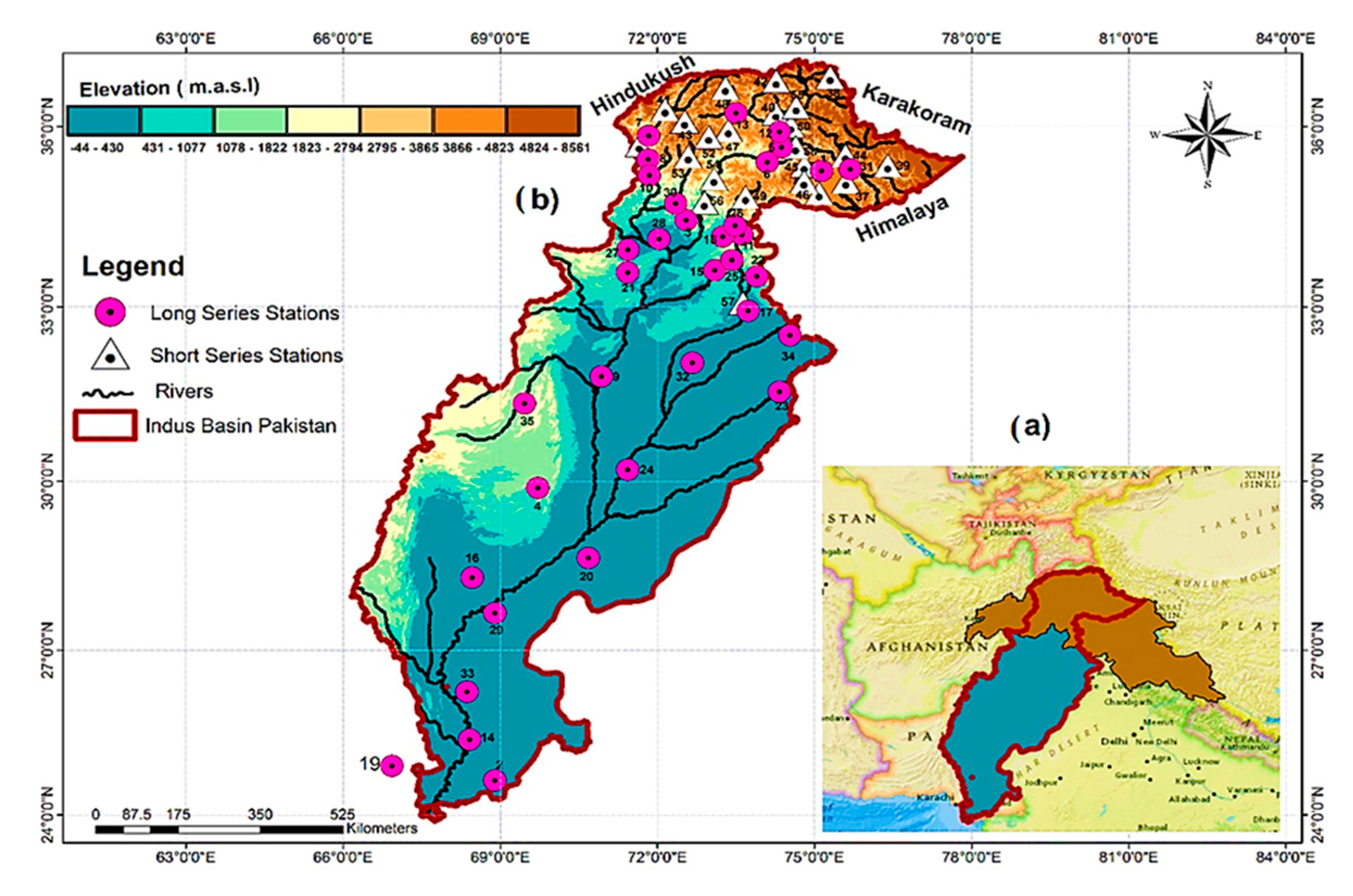
2. Study Area
3. Data and Methodology
3.1. Predictand Data
3.2. Predictor Data
3.3. Statistical Modeling Framework
3.4. GCMs: Predictor-Based Downscaling
3.5. GCM Ranking for Uncertainty Quantification
3.6. Reference Uncertainty
4. Results and Discussion
4.1. Governing Predictors
4.2. Statistical Performance of Downscaling Models
4.3. Quantifying Uncertainties
4.3.1. Reference Uncertainty
4.3.2. Model Uncertainty
4.4. Future Temperature Changes
4.4.1. WS Projections
4.4.2. PMS Projections
4.4.3. MS Projections
4.5. Model Weighting Influence on Ensemble Signals
4.6. Projected Change Signals: Robustness
4.7. Downscaling over the HA-UIB
5. Further Discussion and Conclusions
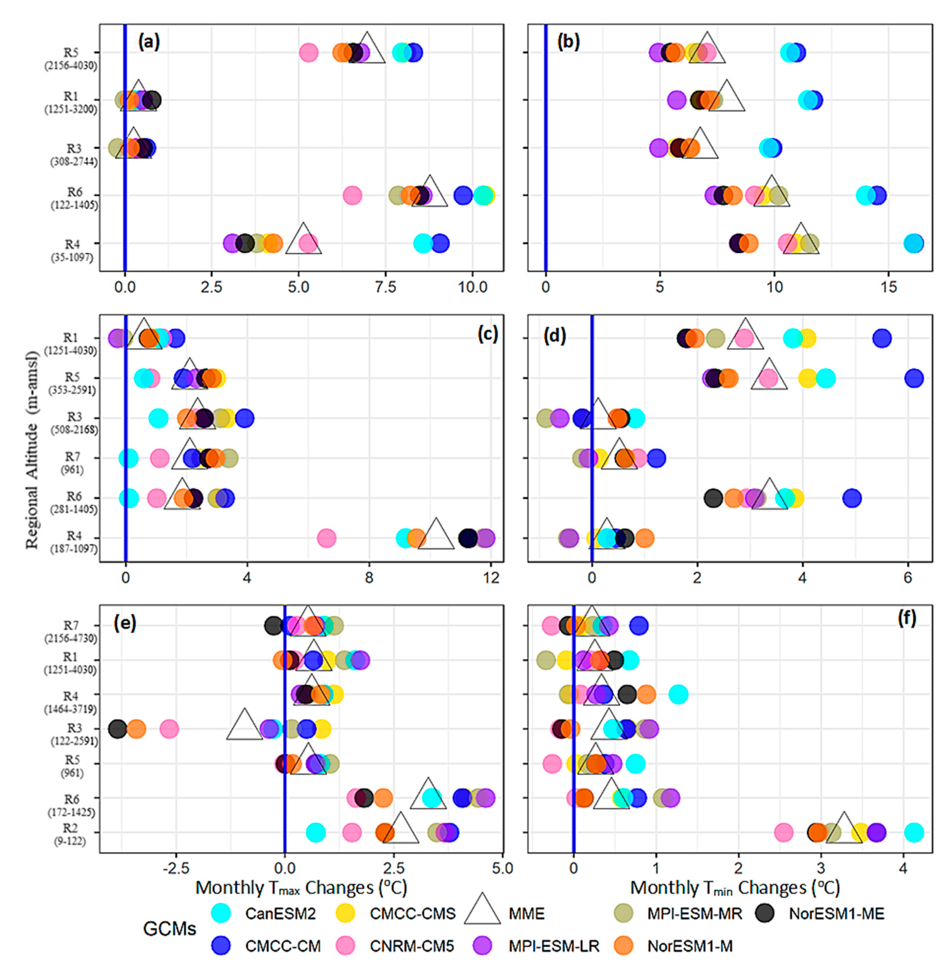
- The entire basin will non-uniformly (space-time scales) warm during the 21st century under both RCPs. The projected warming is strong under RCP8.5 forcing and during 2071–2100 but follows complex patterns.
- The WS showed maximum warming dominated by Tmin changes. The changes suggested an EDW (only for Tmax) and a significant reduction in DTR over the UIB. However, high-altitude regions showed a stable DTR.
- PMS warming was spatially more uniform and instead dominated by Tmax changes. Projected patterns within the UIB suggested a decreasing (increasing) DTR over high-altitudes (low-altitudes) through Tmin (Tmax) changes.
- A remarkable low-warming (inter-model) consensus, particularly over the UIB, appeared during the MS. The projected changes suggested a small increase in seasonal TDR over the UIB, driven mainly by the Tmax changes.
- Over the seasons, a strong (weak) warming appeared over the northwestern high-altitude (lower- elevations of the southern Himalayans) regions. In addition, the increased warming during the westerly-dominated seasons seems to mask low-warming MS patterns over the UIB. Thus, the UIB will experience substantial warming for mean temperature that follows EDW- a pattern consistent with earlier studies e.g., [38]. High warming during the post-monsoon period, e.g., [40], may further increase year-round heating (MS masking) over the UIB.
- Increased inter-model spread within the UIB indicated more uncertainty about ensemble warming and the possibility of even greater PMS (up to 4 °C) and MS (up to 1 °C) warming for both temperatures. Better performing GCMs further confirmed higher warming compared to MMEs signals. Such uncertainties highlight the terrain complexities and observational lackings.
- Contrary to the UIB, the projected warming over different Lower Indus regions (with more uncertainty) was in line with those studies that implemented basin-wide analysis, e.g., [4,77]. A combination of simplified topography (lesser interpolation errors) and reduced need for lapse rates may govern such warming similarities. These regions have a stronger mesoscale land-atmosphere coupling, e.g., [83], which CMIP5 models may not adequately represent due to coarser resolution. Hence more uncertainty prevails over the Lower Indus. The projected precipitation decrease, e.g., [63,77], strengthening of future land-atmosphere coupling, and more decisive influence of the warming oceans in the southwestern and southern regions may largely explain the warming patterns and uncertainty in Lower Indus regions.
Supplementary Materials
Author Contributions
Funding
Institutional Review Board Statement
Data Availability Statement
Acknowledgments
Conflicts of Interest
Appendix A. GCM Ranking and Model Uncertainty
- (I)
- Initially, S-mode PCA is performed (Section 3.2) on every governing predictor (Table 1) of the individual GCMs to extract the same number of PCs as from ERA-Interim.
- (II)
- Subsequently, the model PC loadings are compared with corresponding ERA-Interim loadings (separately for each GCM) using Taylor diagrams (Taylor, 2001). A simple performance score (PS) derived by using two of the three summary statistics of the Taylor diagrams is developed to quantify the correspondence. Mathematically, the PS iswherePS = performance score. For a perfect predictor agreement, PS = 1CR = pattern correlation between the reference (ERA-Interim) and model (GCM) loadings. For a perfect phase match, CR = 1.NSD = normalized ratio of variance (standard deviation of the reference and model loadings). Ideally, the NSD should also take the value 1.Under ideal conditions, the PS will attain its maximum value due to the maximization of phase correspondence (i.e., CR = 1) and the same magnitude of predictor spread (i.e., the term NSD—1 becomes zero) between the reference and model simulations. Similarly, a smaller PS value will show a weaker predictor correspondence. The magnitude of the PS will also intuitively influence the third summary statistics (i.e., standardized RMSE), where its maximum value (PS = 1) will ensure zero error. Conversely, the smaller values (PS < 1) will reflect higher errors, though not following a clear linear trend due to the typical relationships among these three summary statistics, see [72]. Thus, the PS contains useful information about the strength of correspondence between the reference and model-simulated fields and can be used to identify the best-matching pairs for every governing predictor.
- (III)
- We draw two separate sets of Taylor diagrams for each precipitation region and season. The first set of diagrams uses PS to identify the best PC match between reference and modeled PCs of a given predictor (separately for each GCM). In this context, we evaluate all modeled loadings of a predictor against a reference loading. The reference-model pair, which shows the highest PS, is selected as the best GCM-PC for that particular reference.This process is repeated for all other PCs and predictors that appear in the final regression models used for downscaling. Subsequently, all best-matching (individual) PCs of different predictors are grouped into the second set of Taylor diagrams (separately for each GCM) to assess the ability of the GCMs in representing ERA-Interim precipitation predictors over a region. The summary statistics of the second Taylor diagram is used to compute the average PS for each GCM and is termed as unweighted PS due to equal weighting of each PC in its computation.
- (IV)
- Given that each PC has a different influence in a regression model, we adapted (absolute) regression coefficients of the PCs as weights and computed the weighted PS. Thus, a model with the highest (lowest) weighted PS score can be identified as the best (worst) GCM due to its improved (poor) simulations for more important predictors.
- (V)
- This process (step I to IV) is repeated for all sub-regions to identify the best regional GCM in different seasons.Finally, we consider GCM performance over multiple regions to identify models that show superior simulations over the whole spatial scales of the UIB and LI, respectively. We prefer a GCM that performs well in multiple regions. This spatial consideration is important since an outlier may strongly influence the PS of a model (e.g., very high PS just over one sub-region). Source: [43].
References
- IPCC. Summary for Policymakers. In Global Warming of 1.5°C. An IPCC Special Report on the Impacts of Global Warming of 1.5 °C above Pre-industrial Levels and Related Global Greenhouse Gas Emission Pathways, in the Context of Strengthening the Global Response to the Threat of Climate Change, Sustainable Development, and Efforts to Eradicate Poverty; World Meteorological Organization: Geneva, Switzerland, 2018; p. 32. [Google Scholar]
- IPCC. Climate Change 2013: The Physical Science Basis. In Contribution of Working Group I to the Fifth Assessment Report of the Intergovernmental Panel on Climate Change; Stocker, T.F., Qin, D., Plattner, G.-K., Tignor, M., Allen, S.K., Boschung, J., Nauels, A., Xia, Y., Bex, V., Midgley, P.M., Eds.; Cambridge University Press: Cambridge, UK; New York, NY, USA, 2013; p. 1535. [Google Scholar]
- Giorgi, F.; Raffaele, F.; Coppola, E. The response of precipitation characteristics to global warming from climate projections. Earth Syst. Dyn. 2019, 10, 73–89. [Google Scholar] [CrossRef]
- Su, B.; Huang, J.; Gmmer, M.; Jian, D.; Tao, H.; Jiang, T.; Zhao, C. Statistical downscaling of CMIP5 muli-model en-semble for projected changes of climate in the Indus River Basin. Atmos. Res. 2016, 178, 138–149. [Google Scholar] [CrossRef]
- Karmalkar, A.V.; Bradley, R.S. Consequences of Global Warming of 1.5 °C and 2 °C for Regional Temperature and Precipitation Changes in the Contiguous United States. PLoS ONE 2017, 12, e0168697. [Google Scholar] [CrossRef]
- Sutton, R.T.; Dong, B.; Gregory, J.M. Land/sea warming ratio in response to climate change: IPCC AR4 model results and comparison with observations. Geophys. Res. Lett. 2007, 34, 02701. [Google Scholar] [CrossRef]
- Mountain Research Initiative EDW Working Group; Pepin, N.; Bradley, R.S.; Diaz, H.F.; Baraer, M.; Caceres, E.B.; Forsythe, N.; Fowler, H.J.; Greenwood, G.; Hashmi, M.Z.; et al. Elevation-dependent warming in mountain regions of the world. Nat. Clim. Chang. 2015, 5, 424–430. [Google Scholar] [CrossRef]
- Kumar, P.; Saharwardi, S.; Banerjee, A.; Azam, M.F.; Dubey, A.K.; Murtugudde, R. Snowfall Variability Dictates Glacier Mass Balance Variability in Himalaya-Karakoram. Sci. Rep. 2019, 9, 18192. [Google Scholar] [CrossRef]
- Bolch, T.; Kulkarni, A.; Kääb, A.; Huggel, C.; Paul, F.; Cogley, J.G.; Frey, H.; Kargel, J.S.; Fujita, K.; Scheel, M.; et al. The State and Fate of Himalayan Glaciers. Science 2012, 336, 310–314. [Google Scholar] [CrossRef]
- Azam, M.F.; Ramanathan, A.; Wagnon, P.; Vincent, C.; Linda, A.; Berthier, E.; Sharma, P.; Mandal, A.; Angchuk, T.; Singh, V.; et al. Meteorological conditions, seasonal and annual mass balances of Chhota Shigri Glacier, western Himalaya, India. Ann. Glaciol. 2016, 57, 328–338. [Google Scholar] [CrossRef]
- Immerzeel, W.W.; Pellicciotti, F.; Bierkens, M.F.P. Rising river flows throughout the twenty-first century in two Himalayan glacierized watersheds. Nat. Geosci. 2013, 6, 742–745. [Google Scholar] [CrossRef]
- Pritchard, H.D. Asia’s glaciers are a regionally important buffer against drought. Nat. Cell Biol. 2017, 545, 169–174. [Google Scholar] [CrossRef]
- Bolch, T.; Pieczonka, T.; Mukherjee, K.; Shea, J.M. Brief communication: Glaciers in the Hunza catchment (Karakoram) have been nearly in balance since the 1970s. Cryosphere 2017, 11, 531–539. [Google Scholar] [CrossRef]
- Lutz, A.F.; Immerzeel, W.W.; Shrestha, A.B.; Bierkens, M.F.P. Consistent increase in high Asia’s runoff due to increasing glacier melt and precipitation. Nat. Clim. Chang. 2014, 4, 587–592. [Google Scholar] [CrossRef]
- De Souza, K.; Kituyi, E.; Harvey, B.; Leone, M.; Murali, K.S.; Ford, J. Vulnerability to climate change in three hot spots in Africa and Asia: Key issues for policy-relevant adaptation and resilience-building research. Reg. Environ. Chang. 2015, 15, 747–753. [Google Scholar] [CrossRef]
- De Kok, R.J.; Tuinenburg, O.A.; Bonekamp, P.N.J.; Immerzeel, W.W. Irrigation as a Potential Driver for Anomalous Glacier Behavior in High Mountain Asia. Geophys. Res. Lett. 2018, 45, 2047–2054. [Google Scholar] [CrossRef]
- WGMS. Global Glacier Change Bulletin No. 3 (2016–2017); Publication Based on Database Version; World Glacier Monitoring Service: Zurich, Switzerland, 2020; p. 274. [Google Scholar] [CrossRef]
- Zemp, M.; Huss, M.; Thibert, E.; Eckert, N.; McNabb, R.W.; Huber, J.; Barandun, M.; Machguth, H.; Nussbaumer, S.U.; Gärtner-Roer, I.; et al. Global glacier mass changes and their contributions to sea-level rise from 1961 to 2016. Nature 2019, 568, 382–386. [Google Scholar] [CrossRef]
- Brun, F.; Berthier, E.; Wagnon, P.; Kääb, A.; Treichler, D. A spatially resolved estimate of High Mountain Asia glacier mass balances from 2000 to 2016. Nat. Geosci. 2017, 10, 668–673. [Google Scholar] [CrossRef]
- Hewitt, K. The Karakoram anomaly? Glacier expansion and the ‘elevation effect,’ Karakoram Himalaya. Mt. Res. Dev. 2005, 25, 332–340. [Google Scholar] [CrossRef]
- Sakai, A.; Fujita, K. Contrasting glacier responses to recent climate change in high-mountain Asia. Sci. Rep. 2017, 7, 13717. [Google Scholar] [CrossRef]
- Azam, M.F.; Wagnon, P.; Berthier, E.; Vincent, C.; Fujita, K.; Kargel, J.S. Review of the status and mass changes of Himalayan-Karakoram glaciers. J. Glaciol. 2018, 64, 61–74. [Google Scholar] [CrossRef]
- Fowler, H.J.; Archer, D.R. Conflicting signals of climate change in the Upper Indus basin. J. Clim. 2006, 19, 4276–4293. [Google Scholar] [CrossRef]
- Shrestha, A.B.; Wake, C.; Mayewski, P.A.; Dibb, J.E. Maximum temperature trends in the Himalaya and its vi-cinity: Analysis based on temperature records from Nepal for the period 1971–1994. J. Clim. 1999, 12, 2276–2286. [Google Scholar] [CrossRef]
- Kattel, D.B.; Yao, T.; Yang, K.; Tian, L.; Yang, G.; Joswiak, D. Temperature lapse rate in complex mountain terrain on the southern slope of the Central Himalayas. Theor. Appl. Climatol. 2013, 113, 671–682. [Google Scholar] [CrossRef]
- Nayava, J.L.; Adhikary, S.; Bajracharya, O.R. Spatial and temporal variation of surface air temperature at different altitude zone in recent 30 years over Nepal. Mausam 2017, 683, 417–428. [Google Scholar]
- Karl, T.R.; Jones, P.D.; Knight, R.W.; Kukla, G.; Plummer, N.; Razuvayev, V.; Gallo, K.P.; Lindseay, J.; Charlson, R.J.; Peterson, T.C. A new perspective on recent global warming—Asymmetric trends of daily maximum and minimum temperature. Bull. Am. Meteorol. Soc. 1993, 74, 1007–1023. [Google Scholar] [CrossRef]
- Jones, P.D.; New, M.; Parker, D.E.; Martin, S.; Rigor, I.G. Surface air temperature and its changes over the past 150 years. Rev. Geophys. 1999, 37, 173–199. [Google Scholar] [CrossRef]
- Tong, S.; Li, X.; Zhang, J.; Bao, Y.; Bao, Y.; Na, L.; Si, A. Spatial and temporal variability in extreme temperature and precipitation events in Inner Mongolia (China) during 1960–2017. Sci. Total Environ. 2019, 649, 75–89. [Google Scholar] [CrossRef]
- Panda, D.K.; Mishra, A.; Kumar, A.; Mandal, K.; Thakur, A.K.; Srivastava, R.C. Spatiotemporal patterns in the mean and extreme temperature indices of India, 1971-2005. Int. J. Clim. 2014, 34, 3585–3603. [Google Scholar] [CrossRef]
- Miller, J.D.; Immerzeel, W.W.; Rees, G. Climate change impacts on glacier hydrology and river discharge in the Hindukush-Himalayas. Mt. Res. Dev. 2012, 32, 461–467. [Google Scholar] [CrossRef]
- Latif, Y.; Yao, M.; Yaseen, M.; Muhammad, S.; Wazir, M.A. Spatial analysis of temperature time series over the Upper Indus Basin (UIB) Pakistan. Theor. Appl. Clim. 2019, 139, 741–758. [Google Scholar] [CrossRef]
- Yaseen, M.; Ahmad, I.; Guo, J.; Azam, M.I.; Latif, Y. Spatiotemporal Variability in the Hydrometeorological Time-Series over Upper Indus River Basin of Pakistan. Adv. Meteorol. 2020, 2020, 5852760. [Google Scholar] [CrossRef]
- Rajbhandari, R.; Shrestha, A.B.; Kulkarni, A.; Patwardhan, S.K.; Bajracharya, S.R. Projected changes in climate over the Indus river basin using a high resolution regional climate model (PRECIS). Clim. Dyn. 2014, 44, 339–357. [Google Scholar] [CrossRef]
- Khattak, M.; Babel, M.; Sharif, M. Hydro-meteorological trends in the upper Indus River basin in Pakistan. Clim. Res. 2011, 46, 103–119. [Google Scholar] [CrossRef]
- Hasson, S.U.; Böhner, J.; Lucarini, V. Prevailing climatic trends and runoff response from Hindukush–Karakoram–Himalaya, upper Indus Basin. Earth Syst. Dyn. 2017, 8, 337–355. [Google Scholar] [CrossRef]
- Bashir, F.; Zeng, X.; Gupta, H.; Hazenberg, P. A Hydrometeorological Perspective on the Karakoram Anomaly Using Unique Valley-Based Synoptic Weather Observations. Geophys. Res. Lett. 2017, 44, 10470–10478. [Google Scholar] [CrossRef]
- Lutz, A.; Immerzeel, W.W.; Kraaijenbrink, P.D.A.; Shrestha, A.B.; Bierkens, M.F.P. Climate Change Impacts on the Upper Indus Hydrology: Sources, Shifts and Extremes. PLoS ONE 2016, 11, e0165630. [Google Scholar] [CrossRef]
- Ali, S.; Li, D.; Congbin, F.; Khan, F. Twenty first century climatic and hydrological changes over Upper Indus Basin of Himalayan region of Pakistan. Environ. Res. Lett. 2015, 10, 014007. [Google Scholar] [CrossRef]
- Ali, S.; Kiani, R.S.; Reboita, M.S.; Dan, L.; Eum, H.; Cho, J.; Dairaku, K.; Khan, F.; Shreshta, M.L. Identifying hotspots cities vulnerable to climate change in Pakistan under CMIP5 climate projections. Int. J. Clim. 2021, 41, 559–581. [Google Scholar] [CrossRef]
- Khan, F.; Pilz, J.; Ali, S. Improved hydrological projections and reservoir management in the Upper Indus Basin under the changing climate. Water Environ. J. 2017, 31, 235–244. [Google Scholar] [CrossRef]
- Archer, D. Contrasting hydrological regimes in the upper Indus Basin. J. Hydrol. 2003, 274, 198–210. [Google Scholar] [CrossRef]
- Pomee, M.S.; Ashfaq, M.; Ahmad, B.; Hertig, E. Modeling regional precipitation over the Indus River basin of Pakistan using statistical downscaling. Theor. Appl. Clim. 2020, 142, 29–57. [Google Scholar] [CrossRef]
- Ashfaq, M.; Rastogi, D.; Mei, R.; Touma, D.; Leung, L.R. Sources of errors in the simulation of south Asian summer monsoon in the CMIP5 GCMs. Clim. Dyn. 2016, 49, 193–223. [Google Scholar] [CrossRef]
- Sperber, K.R.; Annamalai, H.; Kang, I.-S.; Kitoh, A.; Moise, A.; Turner, A.; Wang, B.; Zhou, T. The Asian summer monsoon: An intercomparison of CMIP5 vs. CMIP3 simulations of the late 20th century. Clim. Dyn. 2013, 41, 2711–2744. [Google Scholar] [CrossRef]
- Cherchi, A.; Annamalai, H.; Masina, S.; Navarra, A. South Asian Summer Monsoon and the Eastern Mediterranean Climate: The Monsoon–Desert Mechanism in CMIP5 Simulations. J. Clim. 2014, 27, 6877–6903. [Google Scholar] [CrossRef]
- Hasson, S.U.; Böhner, J.; Chishtie, F. Low fidelity of CORDEX and their driving experiments indicates future climatic uncertainty over Himalayan watersheds of Indus basin. Clim. Dyn. 2018, 52, 777–798. [Google Scholar] [CrossRef]
- Mishra, V. Climatic uncertainty in Himalayan water towers. J. Geophys. Res. Atmos. 2015, 120, 2689–2705. [Google Scholar] [CrossRef]
- Dars, G.H.; Strong, C.; Kochanski, A.K.; Ansari, K.; Ali, S.H. The Spatiotemporal Variability of Temperature and Precipitation Over the Upper Indus Basin: An Evaluation of 15 Year WRF Simulations. Appl. Sci. 2020, 10, 1765. [Google Scholar] [CrossRef]
- Pritchard, D.M.W.; Forsythe, N.; Fowler, H.J.; O’Donnell, G.M.; Li, X.-F. Evaluation of Upper Indus Near-Surface Climate Representation by WRF in the High Asia Refined Analysis. J. Hydrometeorol. 2019, 20, 467–487. [Google Scholar] [CrossRef]
- Khan, A.J.; Koch, M. Selecting and Downscaling a Set of Climate Models for Projecting Climatic Change for Impact Assessment in the Upper Indus Basin (UIB). Climate 2018, 6, 89. [Google Scholar] [CrossRef]
- Hasson, S.U. Future Water Availability from Hindukush-Karakoram-Himalaya upper Indus Basin under Conflicting Climate Change Scenarios. Climate 2016, 4, 40. [Google Scholar] [CrossRef]
- Akhtar, M.; Ahmad, N.; Booij, M.J. The impact of climate change on the water resources of Hindukush–Karakorum–Himalaya region under different glacier coverage scenarios. J. Hydrol. 2008, 355, 148–163. [Google Scholar] [CrossRef]
- Palazzi, E.; Von Hardenberg, J.; Provenzale, A. Precipitation in the Hindu-Kush Karakoram Himalaya: Observations and future scenarios. J. Geophys. Res. Atmos. 2013, 118, 85–100. [Google Scholar] [CrossRef]
- Immerzeel, W.W.; Wanders, N.; Lutz, A.; Shea, J.M.; Bierkens, M. Reconciling high-altitude precipitation in the upper Indus basin with glacier mass balances and runoff. Hydrol. Earth Syst. Sci. 2015, 19, 4673–4687. [Google Scholar] [CrossRef]
- Trigo, R.M.; Palutikof, J.P. Precipitation Scenarios over Iberia: A Comparison between Direct GCM Output and Different Downscaling Techniques. J. Clim. 2001, 14, 4422–4446. [Google Scholar] [CrossRef]
- Kaspar-Ott, I.; Hertig, E.; Kaspar, S.; Pollinger, F.; Ring, C.; Paeth, H.; Jacobeit, J. Weights for general circulation models from CMIP3/CMIP5 in a statistical downscaling framework and the impact on future Mediterranean precipitation. Int. J. Clim. 2019, 39, 3639–3654. [Google Scholar] [CrossRef]
- Mahmood, R.; Babel, M.S. Evaluation of SDSM developed by annual and monthly sub-models for downscaling temperature and precipitation in the Jhelum basin, Pakistan and India. Theor. Appl. Clim. 2013, 113, 27–44. [Google Scholar] [CrossRef]
- Taylor, K.E.; Stouffer, R.J.; Meehl, G.A. An Overview of CMIP5 and the Experiment Design. Bull. Am. Meteorol. Soc. 2012, 93, 485–498. [Google Scholar] [CrossRef]
- Dahri, Z.H.; Moors, E.; Ludwig, F.; Ahmad, S.; Khan, A.; Ali, I.; Kabat, P. Adjustment of measurement errors to reconcile precipitation distribution in the high-altitude Indus basin. Int. J. Clim. 2018, 38, 3842–3860. [Google Scholar] [CrossRef]
- Hewitt, K. The Snow and Ice Hydrology Project: Research and training for water resource development in the Upper Indus Basin. J. Can. Pak. Coop. 1988, 2, 63–72. [Google Scholar]
- Khan, A.; Naz, B.S.; Bowling, L.C. Separating snow, clean and debris covered ice in the Upper Indus Basin, Hindukush-Karakoram-Himalayas, using Landsat images between 1998 and 2002. J. Hydrol. 2015, 521, 46–64. [Google Scholar] [CrossRef]
- Wilks, S. Statistical Methods in the Atmospheric Sciences; Academic press: Cambridge, MA, USA, 2006; p. 91. [Google Scholar]
- Pomee, M.S.; Hertig, E. Precipitation Projections over the Indus River Basin of Pakistan for the 21st century using a statistical downscaling framework. Int. J. Climatol. 2020. [Google Scholar]
- Wijngaard, J.B.; Tank, A.M.G.K.; Können, G.P. Homogeneity of 20th century European daily temperature and precipitation series. Int. J. Clim. 2003, 23, 679–692. [Google Scholar] [CrossRef]
- Dee, D.P.; Uppala, S.M.; Simmons, A.J.; Berrisford, P.; Poli, P.; Kobayashi, S.; Andrae, U.; Balmaseda, M.A.; Balsamo, G.; Bauer, P.; et al. The ERA-Interim reanalysis: Configuration and performance of the data assimilation system. Q. J. R. Meteorol. Soc. 2012, 137, 553–597. [Google Scholar] [CrossRef]
- Hersbach, H.; de Rosnay, P.; Bell, B.; Schepers, D.; Simmons, A.; Soci, C.; Abdalla, S.; Alonso-Balmaseda, M.; Balsamo, G.; Bechtold, P.; et al. Operational Global Reanalysis: Progress, Future Directions and Synergies with NWP, ERA-Report, 2018, Serie 27. Available online: https://www.ecmwf.int/node/18765 (accessed on 13 November 2019).
- Preisendorfer, R. Principal Component Analysis in Meteorology and Oceanography; Elsevier: Amsterdam, The Netherlands, 1988; p. 42. [Google Scholar]
- Philipp, A. Zirkulationsdynamische Telekonnektivität des Sommerniederschlags im Südhemisphärischen Afrika. Ph.D. Thesis, Bayerische Julius-Maximilians-Universität Würzburg, Würzburg, Germany, 2003. [Google Scholar]
- Sanford, T.J.; Frumhoff, P.C.; Luers, A.; Gulledge, J. The climate policy narrative for a dangerously warming world. Nat. Clim. Chang. 2014, 4, 164–166. [Google Scholar] [CrossRef]
- Von Storch, H.; Zwiers, F.W. Statistical Analysis in Climate Research; Amsterdam University Press: Amsterdam, The Netherlands, 1984; Volume 484. [Google Scholar]
- Taylor, K.E. Summarizing multiple aspects of model performance in a single diagram. J. Geophys. Res. Atmos. 2001, 106, 7183–7192. [Google Scholar] [CrossRef]
- Kalnay, E.; Kanamitsu, M.; Kistler, R.; Collins, W.; Deaven, D.; Gandin, L.; Iredell, M.; Saha, S.; White, G.; Woollen, J.; et al. The NCEP/NCAR 40-year reanalysis project. Bull. Am. Meteorol. Soc. 1996, 77, 437–471. [Google Scholar] [CrossRef]
- Cannon, F.; Carvalho, L.M.; Jones, C.; Norris, J. Winter westerly disturbance dynamics and precipitation in the western Himalaya and Karakoram: A wave-tracking approach. Theor. Appl. Clim. 2015, 125, 27–44. [Google Scholar] [CrossRef]
- Forsythe, N.; Hardy, A.J.; Fowler, H.J.; Blenkinsop, S.; Kilsby, C.G.; Archer, D.R.; Hashmi, M.Z. A detailed cloud fraction climatology of the upper indus basin and its impli-cations for near-surface air temperature. J. Clim. 2015, 28, 3537–3556. [Google Scholar] [CrossRef]
- Wu, J.; Zha, J.; Zhao, D. Evaluating the effects of land use and cover change on the decrease of surface wind speed over China in recent 30 years using a statistical downscaling method. Clim. Dyn. 2016, 48, 131–149. [Google Scholar] [CrossRef]
- Almazroui, M.; Saeed, S.; Saeed, F.; Islam, M.N.; Ismail, M. Projections of Precipitation and Temperature over the South Asian Countries in CMIP6. Earth Syst. Environ. 2020, 4, 297–320. [Google Scholar] [CrossRef]
- Ali, S.; Eum, H.-I.; Cho, J.; Dan, L.; Khan, F.; Dairaku, K.; Shrestha, M.L.; Hwang, S.; Nasim, W.; Khan, I.A.; et al. Assessment of climate extremes in future projections downscaled by multiple statistical downscaling methods over Pakistan. Atmos. Res. 2019, 222, 114–133. [Google Scholar] [CrossRef]
- Ashfaq, M.; Cavazos, T.; Reboita, M.S.; Torres-Alavez, J.A.; Im, E.-S.; Olusegun, C.F.; Alves, L.; Key, K.; Adeniyi, M.O.; Tall, M.; et al. Robust late twenty-first century shift in the regional monsoons in RegCM-CORDEX simulations. Clim. Dyn. 2020, 1–26. [Google Scholar] [CrossRef]
- Mahmood, R.; Mukand, S.B.; Shaofeng, J.I.A. Assessment of temporal and spatial changes of future climate in the Jhelum river basin, Pakistan and India. Weather Clim. Extrem. 2015, 10, 40–55. [Google Scholar] [CrossRef]
- Cook, E.R.; Krusic, P.J.; Jones, P.D. Dendroclimatic signals in long tree-ring chronologies from the Himalayas of Nepal. Int. J. Clim. 2003, 23, 707–732. [Google Scholar] [CrossRef]
- Nath, R.; Luo, Y.; Chen, W.; Cui, X. On the contribution of internal variability and external forcing factors to the Cooling trend over the Humid Subtropical Indo-Gangetic Plain in India. Sci. Rep. 2018, 8, 18047. [Google Scholar] [CrossRef] [PubMed]
- Saeed, F.; Hagemann, S.; Jacob, D.J. Impact of irrigation on the South Asian summer monsoon. Geophys. Res. Lett. 2009, 36, 040625. [Google Scholar] [CrossRef]
- Han, S.; Yang, Z. Cooling effect of agricultural irrigation over Xinjiang, Northwest China from 1959 to 2006. Environ. Res. Lett. 2013, 8, 024039. [Google Scholar] [CrossRef]
- Karki, R.; Hasson, S.U.; Gerlitz, L.; Talchabhadel, R.; Schickhoff, U.; Scholten, T.; Böhner, J. Rising mean and extreme near-surface air temperature across Nepal. Int. J. Clim. 2020, 40, 2445–2463. [Google Scholar] [CrossRef]
- Wilcoxon, F. Individual Comparisons by Ranking Methods. In Breakthroughs in Statistics; Springer: New York, NY, USA, 1945; Volume 1, p. 80. [Google Scholar] [CrossRef]
- Herreid, S.; Pellicciotti, F. The state of rock debris covering Earth’s glaciers. Nat. Geosci. 2020, 13, 1–7. [Google Scholar] [CrossRef]
- Coen, M.C.; Andrews, E.; Aliaga, D.; Andrade, M.; Angelov, H.; Bukowiecki, N.; Ealo, M.; Fialho, P.; Flentje, H.; Hallar, A.G.; et al. Identification of topographic features influencing aerosol observations at high altitude stations. Atmos. Chem. Phys. 2018, 18, 12289–12313. [Google Scholar] [CrossRef]
- Zhao, A.; Bollasina, M.A.; Stevenson, D.S. Strong Influence of Aerosol Reductions on Future Heatwaves. Geophys. Res. Lett. 2019, 46, 4913–4923. [Google Scholar] [CrossRef]
- Wake, C.P. Glaciochemical investigations as a tool for determining the spatial and seasonal variation of snow accumula-tion in the Central Karakoram, northern Pakistan. Ann. Glaciol. 1989, 13, 279–284. [Google Scholar] [CrossRef]
- Myhre, G.; Myhre, C.E.L.; Samset, B.H.; Storelvmo, T. Aerosols and their Relation to Global Climate and Climate Sen-sitivity. Nat. Educ. Knowl. 2013, 4, 7. [Google Scholar]
- Bentsen, M.; Bethke, I.; Debernard, J.B.; Iversen, T.; Kirkevåg, A.; Seland, Ø.; Drange, H.; Roelandt, C.; Seierstad, I.A.; Hoose, C.; et al. The Norwegian Earth System Model, NorESM1-M—Part 1: Description and basic evaluation of the physical climate. Geosci. Model. Dev. 2013, 6, 687–720. [Google Scholar] [CrossRef]
- Knutti, R.; Sedláček, J.; Sanderson, B.M.; Lorenz, R.; Fischer, E.M.; Eyring, V. A climate model projection weighting scheme accounting for performance and interdependence. Geophys. Res. Lett. 2017, 44, 1909–1918. [Google Scholar] [CrossRef]
- Lanzante, J.R.; Dixon, K.W.; Nath, M.J.; Whitlock, C.E.; Adams-Smith, D. Some Pitfalls in Statistical Downscaling of Future Climate. Bull. Am. Meteorol. Soc. 2018, 99, 791–803. [Google Scholar] [CrossRef]
- Palazzi, E.; Von Hardenberg, J.; Terzago, S.; Provenzale, A. Precipitation in the Karakoram-Himalaya: A CMIP5 view. Clim. Dyn. 2014, 45, 21–45. [Google Scholar] [CrossRef]
- Muhammad, S.; Tian, L.; Ali, S.; Latif, Y.; Wazir, M.A.; Goheer, M.A.; Saifullah, M.; Hussain, I.; Shiyin, L. Thin debris layers do not enhance melting of the Karakoram glaciers. Sci. Total. Environ. 2020, 746, 141119. [Google Scholar] [CrossRef]


| Tmax | |||||
|---|---|---|---|---|---|
| Sr. No | Predictors | WS | PMS | MS | Basin-Wide |
| 1 | va200 | 0 | 0 | 0 | 0 |
| 2 | ua200 | 0 | 0 | 0 | 0 |
| 3 | zg200 | 2.4 | 0.0 | 1.3 | 1.4 |
| 4 | zg500 | 0 | 0 | 0 | 0 |
| 5 | zg700 | 0 | 0 | 0 | 0 |
| 6 | hus700 | 0 | 0.0 | 0 | 0 |
| 7 | hur 700 | 0 | 0 | 0 | 0 |
| 8 | hur1000 | 0 | 34.6 | 15.2 | 14.4 |
| 9 | hus1000 | 7.3 | 7.7 | 0 | 3.4 |
| 10 | va500 | 0 | 0 | 45.6 | 24.7 |
| 11 | ua500 | 0 | 0 | 19 | 10.3 |
| 12 | ua700 | 0 | 0 | 0 | 0 |
| 13 | va700 | 0 | 0 | 0 | 0 |
| 14 | va850 | 61 | 42.3 | 10.1 | 30.1 |
| 15 | ua850 | 0 | 0 | 0 | 0.0 |
| 16 | ta850 | 29.3 | 15.4 | 8.9 | 15.8 |
| 17 | psl | 0 | 0 | 0 | |
| Total | 100 | 100 | 100 | 100 | |
| Tmin | |||||
| 1 | va200 | 0 | 0 | 0 | 0 |
| 2 | ua200 | 0 | 0 | 0 | 0 |
| 3 | zg200 | 0 | 0 | 0 | 0 |
| 4 | zg500 | 0 | 0 | 0 | 0 |
| 5 | zg700 | 0 | 0 | 0 | 0 |
| 6 | hus700 | 0 | 0 | 0 | 0 |
| 7 | hur 700 | 0 | 0 | 0 | 0 |
| 8 | hur1000 | 0 | 0 | 0 | 0 |
| 9 | hus1000 | 100 | 34.4 | 8.2 | 26.7 |
| 10 | va500 | 0 | 0 | 44.3 | 25.7 |
| 11 | ua500 | 0 | 21.9 | 0 | 6.7 |
| 12 | ua700 | 0 | 0 | 0. | 0 |
| 13 | va700 | 0 | 25 | 0 | 7.6 |
| 14 | va850 | 0 | 0 | 39.3 | 22.9 |
| 15 | ua850 | 0 | 18.8 | 8.2 | 10.5 |
| 16 | ta850 | 0 | 0 | 0 | 0 |
| 17 | psl | 0 | 0 | 0 | 0 |
| Total | 100 | 100 | 100 | 100 | |
| WS Models | |||||||||||
|---|---|---|---|---|---|---|---|---|---|---|---|
| Region | Reg. Alt | RR | Mean Obs. Tmax | Predictors | PCs | RMSE (°C) | MSESS (%) | R2 | |||
| (m-amsl) | (°C) | (Name) | (Nos) | Cal | Val | Cal | Val | Cal | Val | ||
| R1 | 2223 (1251–3200) | Chilas | 15.16 | va850 | 11 | 1.29 | 1.43 | 84.34 | 80.00 | 0.84 | 0.86 |
| R3 | 1173.5 (308–2744) | Kakul | 15.23 | va850 | 14 | 1.20 | 1.37 | 81.47 | 75.31 | 0.82 | 0.83 |
| R5 | 3266 (2156–4030) | Gupis | 7.79 | temp850 | 6 | 1.36 | 1.46 | 83.78 | 80.75 | 0.84 | 0.85 |
| R4 | 266 (35–1097) | Jacobabad | 25.85 | hus1000 | 3 | 1.25 | 1.30 | 87.62 | 86.32 | 0.88 | 0.89 |
| R6 | 365 (122–1405) | Jehlum | 22.44 | temp850 + zg200 | 7 | 1.35 | 1.50 | 83.27 | 78.39 | 0.83 | 0.86 |
| Avg. Basin | 17.29 | 8 | 1.29 | 1.41 | 84.10 | 80.15 | 0.84 | 0.86 | |||
| Avg. UIB | 12.73 | 10 | 1.28 | 1.42 | 83.20 | 78.69 | 0.83 | 0.85 | |||
| Avg. Lower Indus | 24.15 | 5 | 1.30 | 1.40 | 85.45 | 82.36 | 0.86 | 0.88 | |||
| PMS Models | |||||||||||
| R1 | 2627) (1251–4030) | Astore | 19.97 | va850 | 7 | 1.27 | 1.38 | 90.39 | 88.36 | 0.90 | 0.92 |
| R3 | 1327 (508–2168) | Ghari Duputta | 31.91 | hur1000 + hus1000 | 3 | 1.29 | 1.37 | 91.04 | 89.62 | 0.91 | 0.91 |
| R5 | 1281 (353–2591) | Dir | 27.99 | hur1000 | 3 | 1.36 | 1.41 | 90.00 | 88.83 | 0.90 | 0.91 |
| R7 | 961 (961) | Saidu Sharif | 31.75 | hur1000 | 2 | 1.41 | 1.46 | 89.88 | 88.83 | 0.90 | 0.91 |
| R4 | 419 (187–1097) | Sialkot | 36.64 | temp850 + va850 | 8 | 1.13 | 1.26 | 89.23 | 86.17 | 0.89 | 0.90 |
| R6 | 259 (28–1405) | DI Khan | 38.06 | hur1000 + hus1000 | 3 | 0.98 | 1.05 | 92.75 | 91.40 | 0.93 | 0.93 |
| Avg. Basin | 4 | 1.24 | 1.32 | 90.55 | 88.87 | 0.91 | 0.91 | ||||
| Avg. UIB | 4 | 1.33 | 1.41 | 90.33 | 88.91 | 0.90 | 0.91 | ||||
| Avg. Lower Indus | 6 | 1.06 | 1.16 | 90.99 | 88.79 | 0.91 | 0.92 | ||||
| MS Models | |||||||||||
| R1 | 2218 (1251–4030) | Sakardu | 30.17 | va500 | 13 | 1.16 | 1.33 | 80.10 | 72.47 | 0.80 | 0.82 |
| R3 | 746.25 (122–2591) | Jehlum | 35.08 | hur1000 + va500 + zg200 | 13 | 0.74 | 0.87 | 70.26 | 55.26 | 0.70 | 0.76 |
| R4 | 2868 (1464–3719) | Darosh | 35.27 | ua500 | 10 | 0.94 | 1.08 | 79.83 | 72.42 | 0.80 | 0.82 |
| R5 | 961 (961) | Saidu Sharif | 33.19 | va500 | 11 | 0.78 | 0.90 | 72.08 | 62.05 | 0.72 | 0.77 |
| R7 | 2892.5 (2156–4730) | Gupis | 29.52 | va850 + ua500 | 11 | 1.10 | 1.24 | 84.16 | 79.41 | 0.85 | 0.85 |
| R6 | 659 (172–1425) | Risapur | 36.50 | Temp850 + hur1000 + va850 | 10 | 0.94 | 1.05 | 73.34 | 65.68 | 0.73 | 0.78 |
| R2 | 52 (9–122) | Hyderabad | 36.51 | temp850 + va500 | 11 | 0.67 | 0.74 | 68.33 | 58.81 | 0.68 | 0.72 |
| Avg. Basin | 33.75 | 11 | 0.90 | 1.03 | 75.44 | 66.59 | 0.75 | 0.80 | |||
| Avg. UIB | 32.65 | 12 | 0.94 | 1.08 | 77.29 | 68.32 | 0.77 | 0.80 | |||
| Avg. Lower Indus | 36.51 | 11 | 0.81 | 0.90 | 70.84 | 62.25 | 0.71 | 0.75 | |||
| Seasons | Regions | Tmax | Tmin | Reference Uncertainty (in %) | |||||||
|---|---|---|---|---|---|---|---|---|---|---|---|
| ERA5 | NCEP-II | ERA5 | NCEP-II | Tmax | Tmin | Tmax | Tmin | ||||
| ERA5 | NCEP-II | Range | Range | Range | Range | ||||||
| WS | UIB | ||||||||||
| R1 | 0.83 | 0.66 | 0.95 | 0.69 | 17.00 | 34.00 | 5.00 | 31.00 | 17–34 | 5–31 | |
| R3 | 0.83 | 0.65 | 0.95 | 0.69 | 17.00 | 35.00 | 5.00 | 31.00 | 17–37 | 5–31 | |
| R5 | 0.98 | 0.95 | 0.95 | 0.68 | 2.00 | 5.00 | 5.00 | 32.00 | 2–5 | 5–32 | |
| Avg. over UIB | 0.88 | 0.75 | 0.95 | 0.69 | 12.00 | 24.67 | 5.00 | 31.33 | 12-25 | 5-31 | |
| Lower Indus | |||||||||||
| R4 | 0.94 | 0.68 | 0.94 | 0.69 | 6.00 | 32.00 | 6.00 | 31.00 | 6–32 | 6–31 | |
| R6 | 0.98 | 0.96 | 0.94 | 0.68 | 2.00 | 4.00 | 6.00 | 32.00 | 2-4 | 6-32 | |
| Avg. over Lower Indus | 0.96 | 0.82 | 0.94 | 0.69 | 4.00 | 18.00 | 6.00 | 31.50 | 4–18 | 6–32 | |
| PMS | UIB | ||||||||||
| R1 | 0.85 | 0.88 | 0.74 | 0.63 | 15.00 | 12.00 | 26.00 | 37.00 | 12–15 | 26–42 | |
| R3 | 0.63 | 0.99 | 0.54 | 0.91 | 37.00 | 1.00 | 46.00 | 9.00 | 1–39 | 9–48 | |
| R5 | 0.60 | 0.88 | 0.57 | 0.60 | 40.00 | 12.00 | 43.00 | 40.00 | 12–42 | 42–45 | |
| R7 | 0.59 | 0.59 | 0.53 | 0.59 | 41.00 | 41.00 | 47.00 | 41.00 | 43–43 | 43–49 | |
| Avg. over UIB | 0.67 | 0.84 | 0.60 | 0.68 | 33.25 | 16.50 | 40.50 | 31.75 | 17–35 | 34–42 | |
| Lower Indus | |||||||||||
| R4 | 0.93 | 0.87 | 0.84 | 0.78 | 7.00 | 13.00 | 16.00 | 22.00 | 7–13 | 16–22 | |
| R6 | 0.62 | 0.88 | 0.55 | 0.57 | 38.00 | 12.00 | 45.00 | 43.00 | 12–40 | 45–47 | |
| Avg. over Lower Indus | 0.78 | 0.88 | 0.70 | 0.68 | 22.50 | 12.50 | 30.50 | 32.50 | 13-24 | 32-34 | |
| MS | UIB | ||||||||||
| R1 | 0.78 | 0.64 | 0.83 | 0.77 | 22.00 | 36.00 | 17.00 | 23.00 | 22–36 | 17–23 | |
| R3 | 0.66 | 0.59 | 0.73 | 0.64 | 34.00 | 41.00 | 27.00 | 36.00 | 34–43 | 27–36 | |
| R4 | 0.91 | 0.81 | 0.76 | 0.60 | 9.00 | 19.00 | 24.00 | 40.00 | 9–19 | 24–40 | |
| R5 | 0.74 | 0.64 | 0.79 | 0.58 | 26.00 | 36.00 | 21.00 | 42.00 | 26–38 | 21–42 | |
| R7 | 0.89 | 0.69 | 0.78 | 0.56 | 11.00 | 31.00 | 22.00 | 44.00 | 11–31 | 22–44 | |
| Avg. over UIB | 0.80 | 0.67 | 0.78 | 0.63 | 20.40 | 32.60 | 22.20 | 37.00 | 20–33 | 22–37 | |
| Lower Indus | |||||||||||
| R2 | 0.80 | 0.66 | 0.80 | 0.58 | 20.00 | 34.00 | 20.00 | 42.00 | 20–36 | 20–42 | |
| R6 | 0.71 | 0.62 | 0.72 | 0.65 | 29.00 | 38.00 | 28.00 | 0.35 | 29–40 | 28–35 | |
| Avg. over Lower Indus | 0.76 | 0.64 | 0.76 | 0.62 | 24.50 | 36.00 | 23.05 | 21.18 | 25–38 | 23–39 | |
| Seasons | Regions | CMCC-CMS | CMCC-CM | CNRM-CM5 | Can-ESM2 | MPI-ESM-LR | MPI-ESM-MR | Nor-ESM1-ME | Nor-ESM1-M | Model Ensemble |
|---|---|---|---|---|---|---|---|---|---|---|
| UIB | ||||||||||
| WS | R1 | 0.50 | 0.64 | 0.59 | 0.49 | 0.58 | 0.48 | 0.37 | 0.38 | 0.50 |
| R3 | 0.52 | 0.62 | 0.54 | 0.48 | 0.57 | 0.52 | 0.36 | 0.33 | 0.49 | |
| R5 | 0.80 | 0.90 | 0.83 | 0.84 | 0.91 | 0.90 | 0.81 | 0.76 | 0.84 | |
| Avg. over UIB | 0.61 | 0.72 | 0.65 | 0.60 | 0.69 | 0.63 | 0.51 | 0.49 | 0.61 | |
| UIB Uncertainity (in %) | 39.33 | 28 | 34.67 | 39.67 | 31.33 | 36.67 | 48.67 | 51 | 38.67 | |
| Lower Indus | ||||||||||
| R4 | 0.71 | 0.76 | 0.81 | 0.72 | 0.63 | 0.64 | 0.62 | 0.65 | 0.69 | |
| R6 | 0.78 | 0.88 | 0.79 | 0.84 | 0.88 | 0.89 | 0.79 | 0.75 | 0.83 | |
| Avg. over Lower Indus | 0.75 | 0.82 | 0.80 | 0.78 | 0.76 | 0.77 | 0.71 | 0.70 | 0.76 | |
| Lower Indus Uncertainity (in %) | 25.50 | 18 | 20 | 22 | 24.50 | 23.50 | 29.50 | 30 | 24.13 | |
| PMS | UIB | |||||||||
| R1 | 0.59 | 0.62 | 0.56 | 0.60 | 0.65 | 0.61 | 0.53 | 0.59 | 0.59 | |
| R3 | 0.65 | 0.74 | 0.77 | 0.43 | 0.76 | 0.65 | 0.50 | 0.48 | 0.62 | |
| R5 | 0.66 | 0.76 | 0.78 | 0.45 | 0.82 | 0.66 | 0.53 | 0.52 | 0.65 | |
| R7 | 0.65 | 0.73 | 0.79 | 0.43 | 0.82 | 0.67 | 0.53 | 0.53 | 0.64 | |
| Avg. over UIB | 0.64 | 0.71 | 0.73 | 0.48 | 0.76 | 0.65 | 0.52 | 0.53 | 0.63 | |
| UIB Uncertainity (in %) | 36.25 | 28.75 | 27.50 | 52.25 | 23.75 | 35.25 | 47.75 | 47 | 37.31 | |
| Lower Indus | ||||||||||
| R4 | 0.58 | 0.64 | 0.69 | 0.65 | 0.66 | 0.72 | 0.58 | 0.63 | 0.64 | |
| R6 | 0.62 | 0.70 | 0.75 | 0.38 | 0.75 | 0.63 | 0.47 | 0.46 | 0.60 | |
| Avg. over Lower Indus | 0.60 | 0.67 | 0.72 | 0.52 | 0.71 | 0.68 | 0.53 | 0.55 | 0.62 | |
| Lower Indus Uncertainity (in %) | 40 | 33 | 28 | 48.50 | 29.50 | 32.50 | 47.50 | 45.50 | 38.06 | |
| MS | UIB | |||||||||
| R1 | 0.38 | 0.39 | 0.40 | 0.34 | 0.43 | 0.39 | 0.35 | 0.29 | 0.37 | |
| R3 | 0.49 | 0.50 | 0.53 | 0.51 | 0.53 | 0.56 | 0.45 | 0.54 | 0.51 | |
| R4 | 0.61 | 0.55 | 0.46 | 0.48 | 0.62 | 0.60 | 0.57 | 0.54 | 0.55 | |
| R5 | 0.39 | 0.41 | 0.41 | 0.40 | 0.46 | 0.43 | 0.42 | 0.36 | 0.41 | |
| R7 | 0.60 | 0.58 | 0.51 | 0.50 | 0.61 | 0.55 | 0.44 | 0.43 | 0.53 | |
| Avg. over UIB | 0.49 | 0.49 | 0.46 | 0.45 | 0.53 | 0.51 | 0.45 | 0.43 | 0.48 | |
| UIB Uncertainity (in %) | 50.60 | 51.40 | 53.80 | 55.40 | 47 | 49.40 | 55.40 | 56.80 | 52.48 | |
| Lower Indus | ||||||||||
| R2 | 0.41 | 0.46 | 0.45 | 0.43 | 0.42 | 0.42 | 0.44 | 0.43 | 0.43 | |
| R6 | 0.37 | 0.44 | 0.51 | 0.58 | 0.48 | 0.47 | 0.55 | 0.65 | 0.51 | |
| Avg. over Lower Indus | 0.39 | 0.45 | 0.48 | 0.51 | 0.45 | 0.45 | 0.50 | 0.54 | 0.47 | |
| Lower Indus Uncertainity (in %) | 61 | 55 | 52 | 49.50 | 55 | 55.50 | 50.50 | 46 | 53.06 | |
Publisher’s Note: MDPI stays neutral with regard to jurisdictional claims in published maps and institutional affiliations. |
© 2021 by the authors. Licensee MDPI, Basel, Switzerland. This article is an open access article distributed under the terms and conditions of the Creative Commons Attribution (CC BY) license (http://creativecommons.org/licenses/by/4.0/).
Share and Cite
Pomee, M.S.; Hertig, E. Temperature Projections over the Indus River Basin of Pakistan Using Statistical Downscaling. Atmosphere 2021, 12, 195. https://doi.org/10.3390/atmos12020195
Pomee MS, Hertig E. Temperature Projections over the Indus River Basin of Pakistan Using Statistical Downscaling. Atmosphere. 2021; 12(2):195. https://doi.org/10.3390/atmos12020195
Chicago/Turabian StylePomee, Muhammad Saleem, and Elke Hertig. 2021. "Temperature Projections over the Indus River Basin of Pakistan Using Statistical Downscaling" Atmosphere 12, no. 2: 195. https://doi.org/10.3390/atmos12020195
APA StylePomee, M. S., & Hertig, E. (2021). Temperature Projections over the Indus River Basin of Pakistan Using Statistical Downscaling. Atmosphere, 12(2), 195. https://doi.org/10.3390/atmos12020195