Article

Observations and Simulations of Meteorological Conditions over Arctic Thick Sea Ice in Late Winter during the Transarktika 2019 Expedition

1
Department of Environmental Meteorology, University of Trier, 54286 Trier, Germany
2
Arctic and Antarctic Research Institute (AARI), Air-sea interaction department, 199397 St. Petersburg, Russia
*
Author to whom correspondence should be addressed.
Atmosphere 2021, 12(2), 174; https://doi.org/10.3390/atmos12020174
Submission received: 16 December 2020 / Revised: 25 January 2021 / Accepted: 25 January 2021 / Published: 28 January 2021
(This article belongs to the Section Meteorology)

Abstract

:
The parameterization of ocean/sea-ice/atmosphere interaction processes is a challenge for regional climate models (RCMs) of the Arctic, particularly for wintertime conditions, when small fractions of thin ice or open water cause strong modifications of the boundary layer. Thus, the treatment of sea ice and sub-grid flux parameterizations in RCMs is of crucial importance. However, verification data sets over sea ice for wintertime conditions are rare. In the present paper, data of the ship-based experiment Transarktika 2019 during the end of the Arctic winter for thick one-year ice conditions are presented. The data are used for the verification of the regional climate model COSMO-CLM (CCLM). In addition, Moderate Resolution Imaging Spectroradiometer (MODIS) data are used for the comparison of ice surface temperature (IST) simulations of the CCLM sea ice model. CCLM is used in a forecast mode (nested in ERA5) for the Norwegian and Barents Seas with 5 km resolution and is run with different configurations of the sea ice model and sub-grid flux parameterizations. The use of a new set of parameterizations yields improved results for the comparisons with in-situ data. Comparisons with MODIS IST allow for a verification over large areas and show also a good performance of CCLM. The comparison with twice-daily radiosonde ascents during Transarktika 2019, hourly microwave water vapor measurements of first 5 km in the atmosphere and hourly temperature profiler data show a very good representation of the temperature, humidity and wind structure of the whole troposphere for CCLM.

1. Introduction

The impact of the recent global climate change is most pronounced in the Arctic, where the near-surface warming effects are 2–3 times the global average [1]. This effect, called “Arctic Amplification”, is strongly related to atmosphere–ocean–sea ice (AOI) interactions and their feedbacks between the free atmosphere, the atmospheric boundary layer (ABL) and the surface. The strong reductions in sea ice thickness, volume and the minimum extent have led to a new state, which has been termed the “New Arctic”, where the winter sea ice consists mainly of first year ice [2,3]. On a regional scale, the sea ice changes have led to much larger temperature trends than average trends in the Arctic [4].
In order to understand the New Arctic and its future development, AOI interactions over the Arctic sea ice areas represent key processes. Fractional sea ice cover and the distribution of leads have a large impact on the ABL [5], particularly during winter. While a couple of experiments have been performed in the marginal ice zone and thin ice areas [6], experiments for the inner Arctic representing wintertime conditions with thick ice are rare.
Regional climate models (RCMs) are an important tool to investigate the relevant processes to understand the New Arctic. In order to include effects of topographic winds and polynyas as well as extreme winds in atmospheric models, a horizontal resolution of 15 km or less is needed [7,8]. Global reanalyses (such as ERA-Interim, [9]) and most of the regional climate models used in Arctic CORDEX [10] have coarser resolutions (25–80 km). Parameterization of the stable boundary layer (SBL) and subgrid processes such as leads are major challenges for atmospheric models. In all state-of-the-art RCMs, leads are not realistically represented [11]. Sea ice is considered as a mean concentration over a model grid box, and surface fluxes are computed according to the fractions of water and ice. Most uncoupled RCMs assume open water for the water fraction, which is unrealistic during winter, where leads and polynyas are almost totally covered with thin ice [12]. The thin ice coverage has a large effect on the surface fluxes and sea ice production [13].
In the present paper, we use data of the experiment Transarktika 2019 during April 2019, where the Russian research vessel “R/V Akademik Tryoshnikov” drifted with the ice in the inner Arctic [14]. A meteorological tower was installed on level sea ice at a distance of about 350 m from the ship, and atmospheric remote sensing measurements as well as radiosonde ascents were performed on the ship [15]. The data are used for a verification of the regional climate model COSMO-CLM (CCLM) with a horizontal resolution of 5 km (Figure 1). The sea-ice concentration data are from Advanced Microwave Scanning Radiometer (AMSR2) data [16], and thin-ice thickness (TIT) from Soil Moisture and Ocean Salinity (SMOS) data [17]. Although the ship track came close to a polynya near Franz Josef Land at the end of April (Figure 1), the ship remained in thick ice all the time.

2. Data and Methods

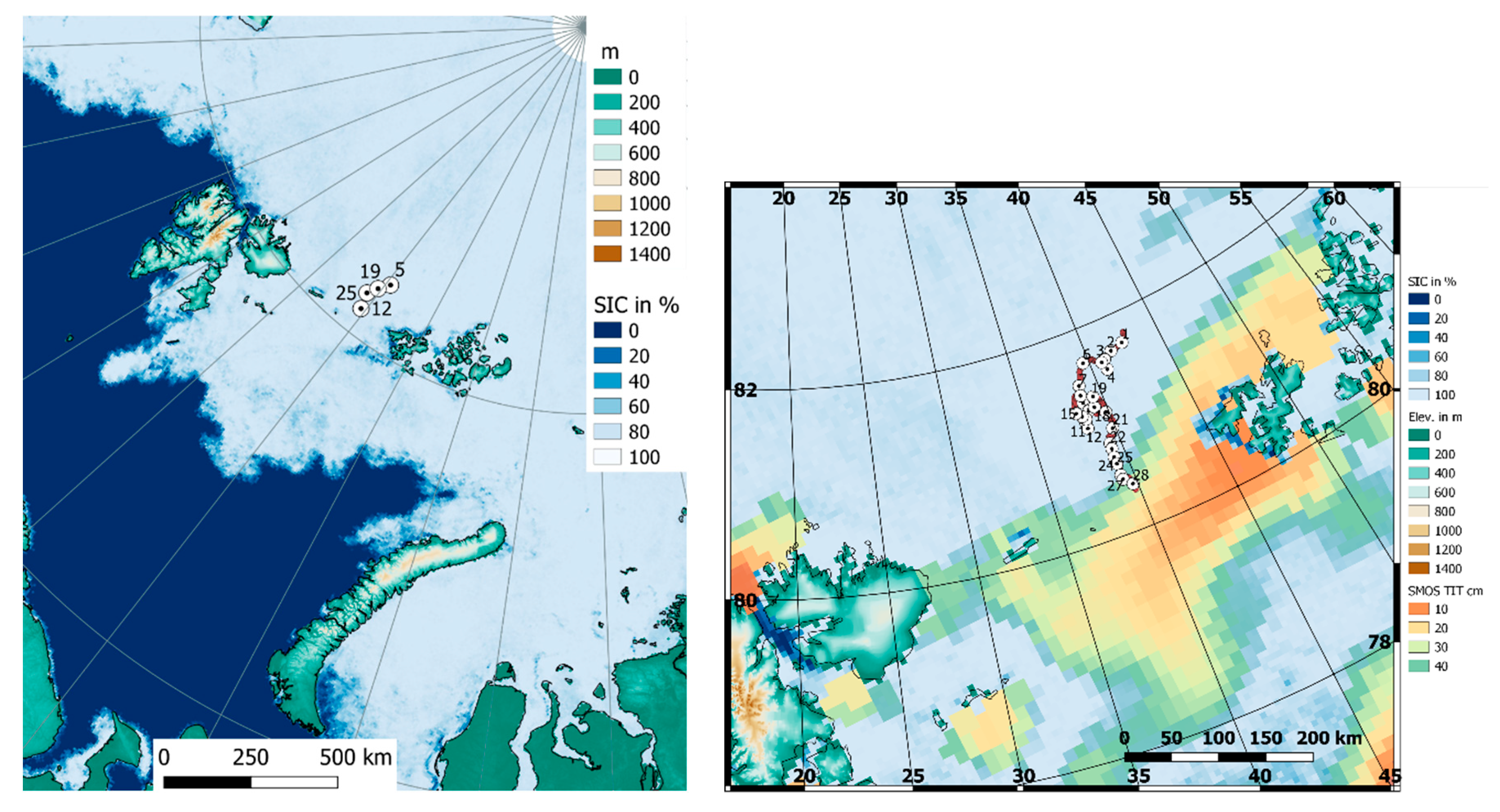
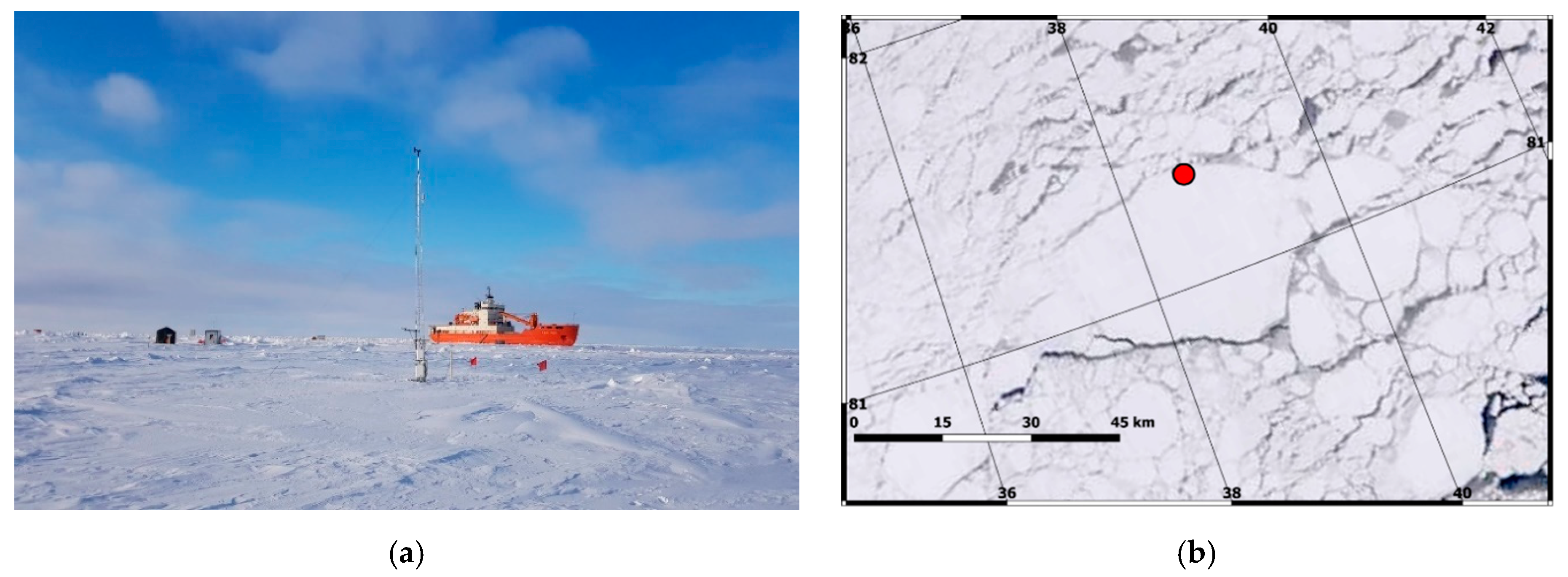
2.1. The Transarktika Experiment

The experiment was performed during April 2019 in the area between Svalbard and Franz Josef Land [14]. During the drift, an area of flat ice located as far as possible from hummocks, frozen leads, cracks and sastrugi was chosen. For security reasons, the equipment was placed compactly in the area of the meteorological site, forming a single multifunctional measuring complex (Figure 2a). The Campbell Scientific (CS) gradient meteorological complex was deployed 100 m from the pavilion, where the measurement data were recorded, and at a distance of 350 m from the vessel. Temperature and relative humidity sensors HMP155A were installed on the mast at heights of 2 and 8 m, anemometers RM Young 05108—at heights of 2 and 10 m. A compass (ComNav), necessary for calculation of true wind direction, was installed on the mast in addition. The four-component radiometer CNR4 was installed at a height of 2 m at a distance of 35 m from the mast. The meteorological temperature profiler MTP5, ceilometer CL-51, and water vapor radiometer RVP were installed on the second open deck of R/V “Akademik Tryoshnikov” at the height 30 m. Radiosoundings were carried out using the radiosounding system “Polyus-M” and sondes MRZ-N1, manufactured by producer “Radiy”. General information about meteorological instrumentation during Transarktika 2019 is presented in Table 1.

2.2. Satellite Data

We use the Moderate Resolution Imaging Spectroradiometer (MODIS) ice surface temperature (IST) product MOD29 (Terra satellite) and MYD29 (Aqua satellite), in the following referred to as MxD29 [18]. The product is used as collection 6 Level-2 swath data, and has a spatial resolution of 1 km at nadir. Daily composites are produced as described in [19,20]. The accuracy of IST data is specified as about 2 K [21]. However, the MODIS cloud mask has deficits and many pixels are still contaminated by clouds, leading to artifacts in the IST data. With the aim of detecting sea-ice leads in the Arctic, the authors of [20,22] have developed an additional cloud filter, which removes most artifacts.

2.3. The CCLM Model

The regional climate model COSMO-CLM (CCLM, used version: COSMO-CLM-v5.0_clm16) is the community model of the German regional climate research community [23]. CCLM has been used for several studies of polynyas (e.g., [13,24,25]). Verification studies for CCLM have been performed, e.g., using standard weather station data [4,26], radiosondes [27] and aircraft data [28]. For the present paper, CCLM is used with a horizontal resolution of 5 km for the Barents and Kara Sea (Figure 1). Initial and boundary data are taken from ERA5 [29,30] with hourly resolution. The model is used in a forecast mode (reinitialized daily at 18:00 UTC, spin-up time of 6 h) for April 2019 (Transarktika period). No nudging is performed. Model output is available every 1 h. In the vertical, the model extends up to 22 km with 60 vertical levels, 12 levels are below 500 m in order to obtain a high resolution of the boundary layer. The first model level is at 5 m above the surface. Sea ice concentration as shown in Figure 1 is taken from AMSR2 data with 6 km resolution [16]. Sea ice thickness is prescribed daily from interpolated Pan-Arctic Ice Ocean Modeling and Assimilation System (PIOMAS) fields [31]. Topography data are taken from [32]. A full technical documentation of the CCLM model can be found in [33]. CCLM was adapted to polar regions by implementing a two-layer sea ice model [34], a tile approach for sea ice [13], and modifications for the stable boundary layer [27,28]. The modifications for the stable boundary layer include a reduction in the lower limit of minimum diffusion coefficients to improve the simulation of the surface inversion over ice surfaces (see Supplementary Material for details). The cloud schemes are described in [35]. The cloud schemes include cloud water, cloud ice, rain, snow and graupel as three-dimensional prognostic variables using a bulk microphysics parameterization scheme. The radiative transfer scheme is described in detail in [36]. It is based on a δ-two-stream solution of the radiative transfer equation and is solved for eight spectral intervals for each model layer considering cloud water droplets, cloud ice crystals, water vapor, ozone, carbon dioxide and other minor trace gases as well as aerosols [35].
Further modifications concerning the sea ice model, the tile approach and the surface layer parameterizations were implemented for the present study and are described in the Supplementary Material in more detail. In summary, these modifications include an improved computation of the sea ice energy budget, a new parameterization of the subgrid-scale ice thickness (thin ice in leads and polynyas), non-linear averaging for the tile approach and new parameterizations for the roughness lengths of momentum and heat.

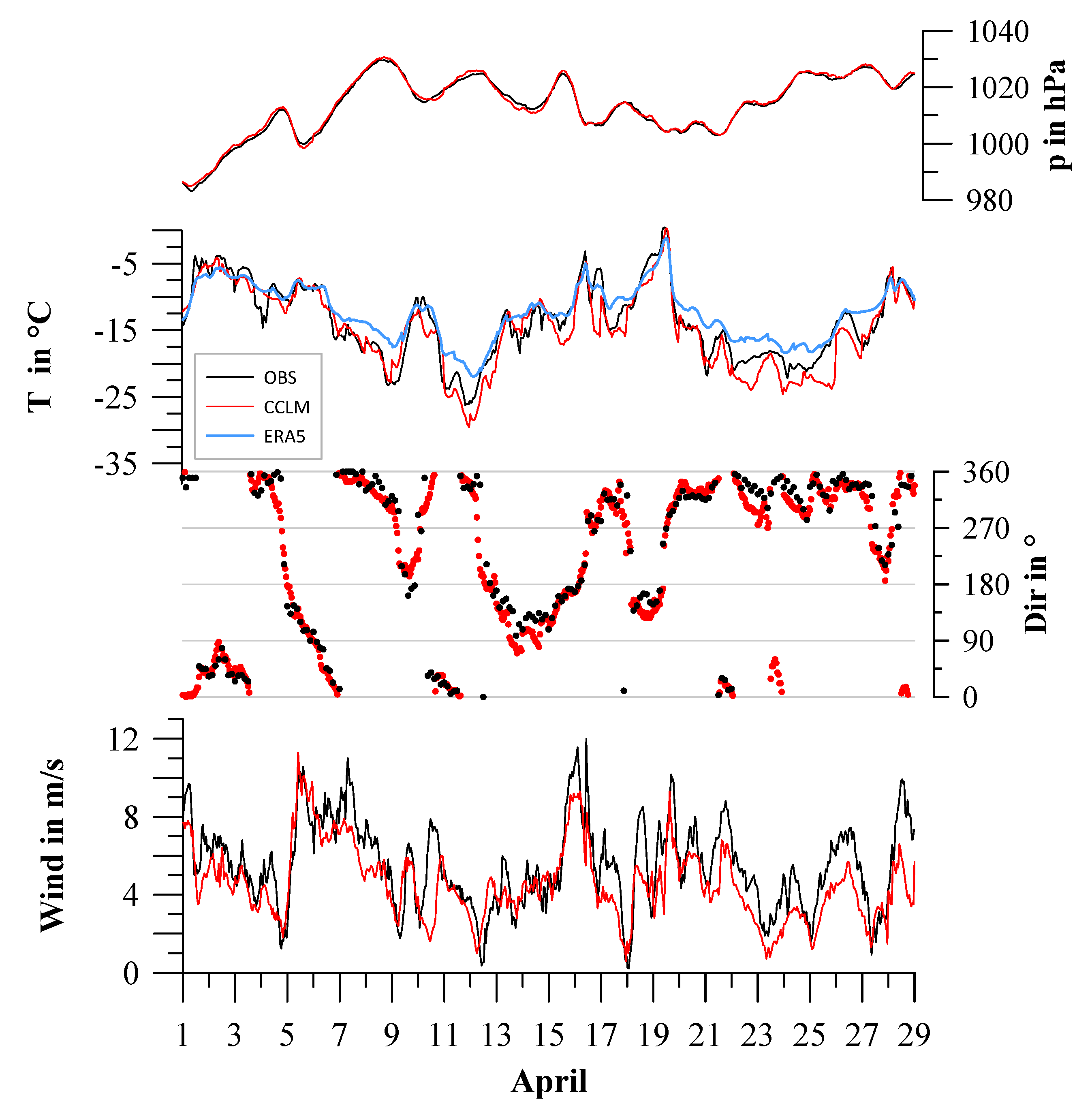
3. Meteorological Conditions during Transarktika 2019

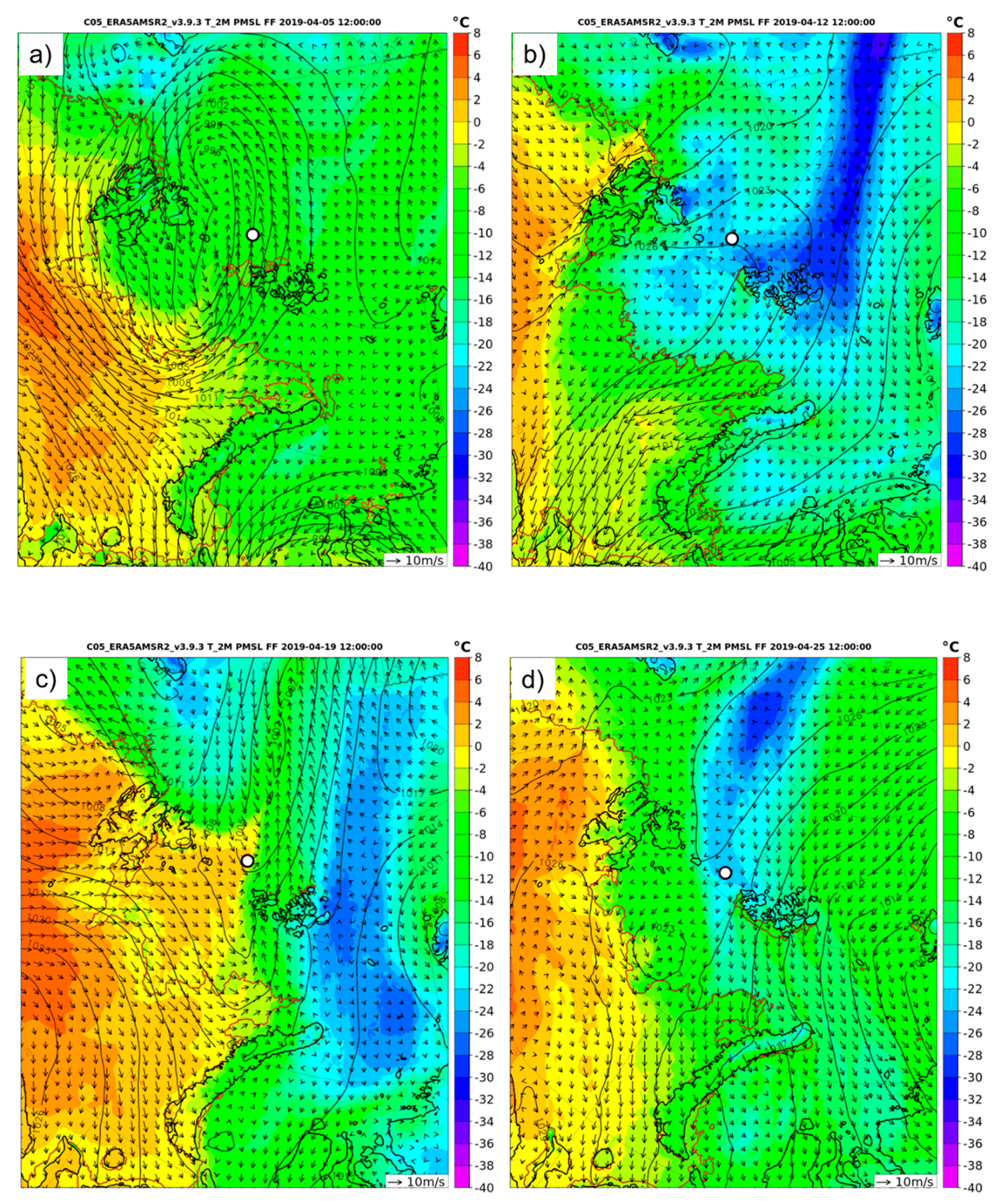
Synoptic Overview over the Measurement Period

The measurements of 10 m wind, 2 m temperature and pressure for 1–29 April are shown in Figure 3 together with the simulation results. Wind speeds are moderate most of the time, but for some periods with cyclonic events the wind speed exceeds 10 m/s (6 and 16 April). The measurements show a weak daily cycle of the temperature for most all days, but also a strong influence of synoptic forcing (e.g., 9–13 April). The coldest temperatures of −25 °C were observed during 11–13 April. The warmest period with up to 0 °C occurred on 19 April. Wind directions were northerly most of the time, but also some remarkable wind direction changes occurred during the passage of cyclones and frontal systems. The simulations agree very well with the measurements indicating some underestimation of the wind speed and slightly too low temperatures.
Figure 4 shows the surface fluxes of downward shortwave and longwave radiation. The daily cycle and amplitude of the shortwave radiation is simulated well with a slight overestimation at the end of April. For the longwave radiation, the tendency for an underestimation can be seen particularly for 22–26 April. Overall, the simulation yields very good results for the radiation fluxes, also for the net radiation (not shown). The statistics of the comparisons are given in the next section.
Figure 5 shows the synoptic conditions as fields of the CCLM simulations for the 2 m temperature, 10 m wind and mean sea level pressure for selected days of April 2019. On 5 April, a low-pressure system lay between Svalbard and Franz Josef Land (FJL). The ship was in the strong wind area east of the low-pressure system with southerly directions, but the wind turned to northerly directions after the passage of the low-pressure system. The lowest temperatures occurred on 12 April, when very weak winds were present in the area of a high-pressure ridge between Svalbard and FJL. The warm event on 19 April is associated with a warm front of a low-pressure system north of the measurement area. A pronounced shift in wind direction from southerly to westerly directions occurs during the passage of this warm front, followed by a cold front with a sharp temperature drop and a shift to northerly flow. On 25 April, a period of relatively cold temperatures occurred, which was associated with weak winds and a high-pressure ridge between Svalbard and FJL. In the monthly average (not shown), a cyclone with the center in the eastern Kara Sea is found for the mean sea-level pressure (MSLP) as well as at 500 hPa, which is consistent with the general northerly wind directions.

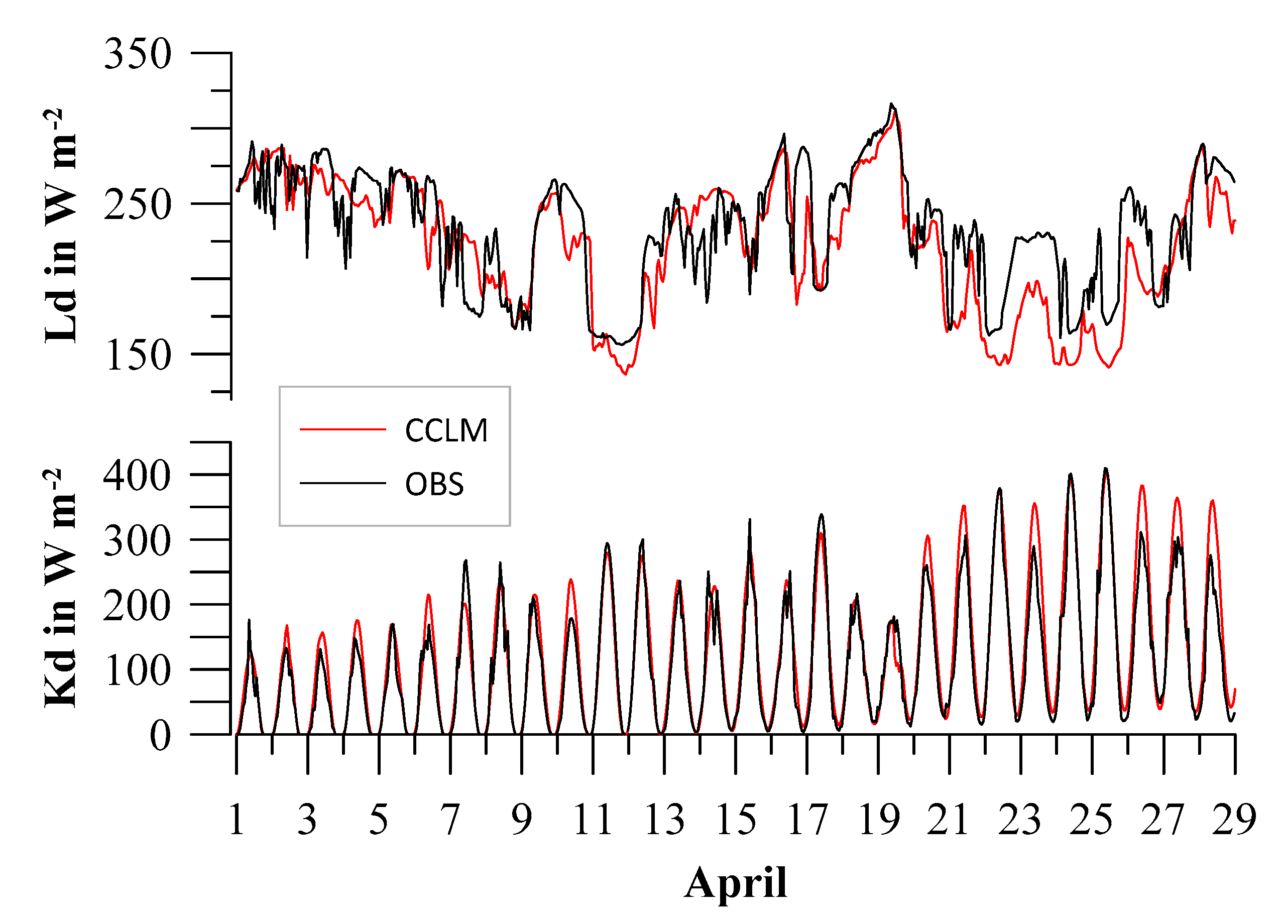
4. Verification for Near-Surface Variables

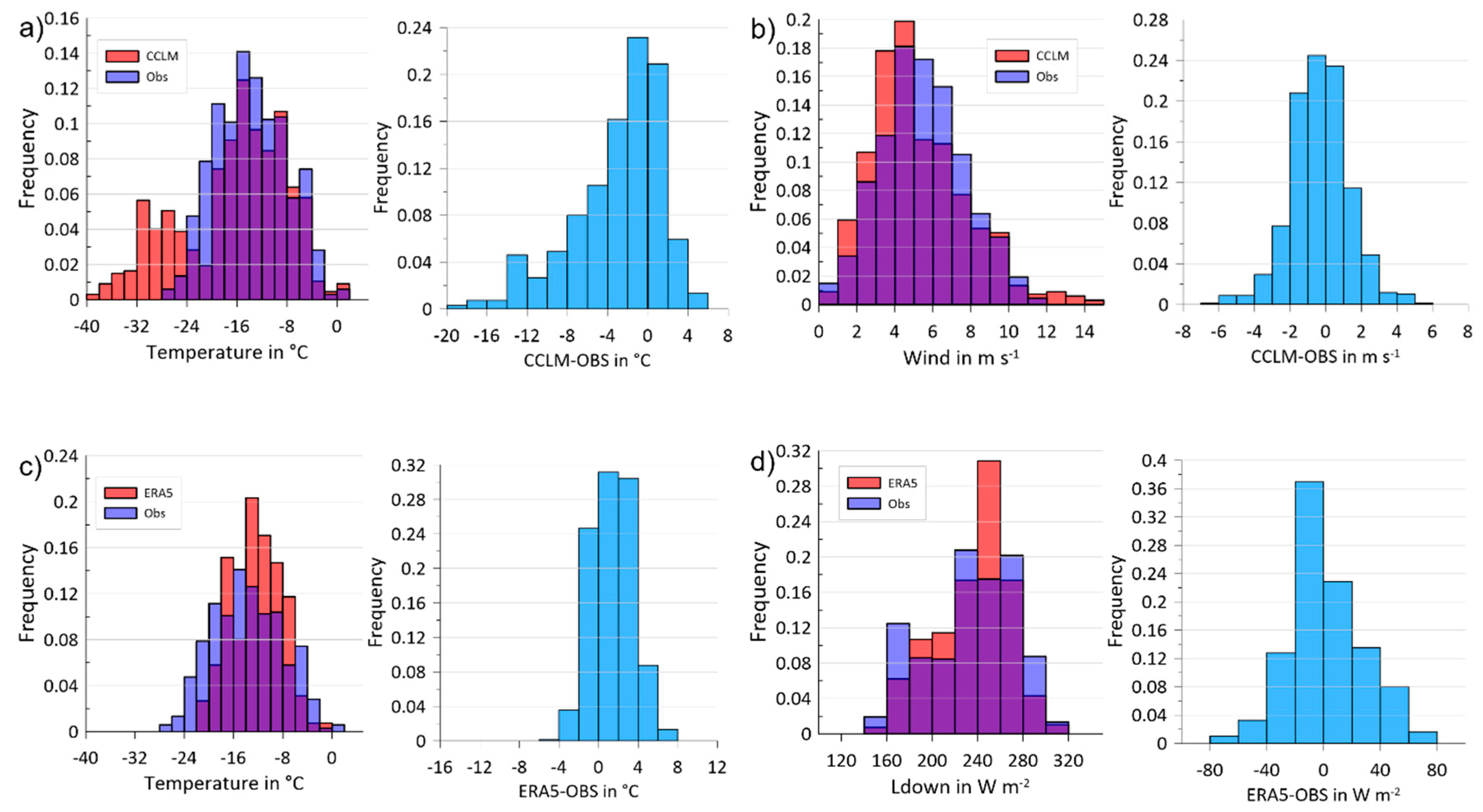
4.1. Statistics for the Comparison with In-Situ Data

The overall statistics of the comparisons for wind, temperature and radiation data are presented in Table 2. For this comparison, data were linearly detrended for the calculation of correlations. Wind speed and temperature show both small biases of −1.0 m/s and −1.1 K, respectively. The pressure is simulated very well with almost no bias, an RMSE smaller than 1 hPa and a correlation exceeding 0.99. Downward shortwave radiation shows a small positive bias and a very good correlation (r = 0.95). For downward longwave radiation, the bias is similar (but negative), and correlation is lower (r = 0.79). The bias for the net radiation is also small, but the correlation (r = 0.63) is not as good as for the incoming radiation fluxes. In order to quantify the daily amplitude, the time series were low-pass filtered using a Gaussian filter with a filter width of 36 h. The daily variations are calculated by subtraction of the low-pass filtered time series from the original time series. As a measure of the mean daily amplitude, the difference between the 90% and 10% percentiles of the daily variations are calculated. As this calculation makes sense only for quantities showing a daily cycle, it is only shown for temperature, downward shortwave and net radiation. The simulated average amplitudes agree very well with the observations (Table 2).
In order to get a more detailed view about the statistics of the comparison, the frequency distribution of measured and simulated values as well as their differences is shown in Figure 6. The negative bias for the temperature is mainly a result of the fact that CCLM simulates temperatures that are too low when temperatures are below −20 °C, while the frequencies of temperatures higher than −6 °C are underestimated. For wind, the frequencies of lower speeds are overestimated by CCLM, and wind speeds above 6 m/s are underestimated. For pressure, the simulation is very good for the whole pressure range, and the difference has a peak for 0–1 hPa. The shortwave radiation is overestimated for very large values with more than 300 W/m2, while values below 40 W/m2 occur more often in the observations. In a few cases, the overestimation is up to more than 100 W/m2, but the peak of the differences is at 0–20 W/m2 (RMSE is 34 W/m2, see Table 2). The longwave radiation is underestimated for the very low values and underestimated for the larger values. Together with the findings for the shortwave radiation, this suggests that CCLM tends to underestimate clouds and the longwave emission for cloud-free conditions. This is also seen in the net radiation, where CCLM shows negative values too frequently and positive values more frequently. For the net radiation, the emission of the surface and the albedo play an additional role. The comparison of the albedo shows that the parameterized albedo in the sea ice model agrees well with the observations most of the time, the largest differences with more than 5% occur during the periods 7–9 April and 21–26 April. For the upward radiation fluxes (and albedo) it has to be taken into account that the measurements represent a specific ice floe, while the model represents a grid scale of 5 km, and it has slightly lower ice concentrations during these two periods (see also discussion section). This makes a comparison of upward radiation fluxes and net radiation more difficult compared to temperature and wind, where a blending of the influences of different surface types in the surroundings of the measurement site occurs.
When using the old version of the sea ice and ABL parameterizations (see Supplementary Material), a distinct underestimation is found at very low temperatures (Figure 7a). The cold bias is −2.9 K and the RMSE is 5.4 K, which is much larger than for the new version. In contrast, the bias in wind speed (−0.3 m/s) is smaller than in the new version, but wind speeds larger than 12 m/s are overestimated (Figure 7b). The statistics for differences between observations and for ERA5 data are shown in Figure 7c for the 2 m temperature. ERA5 simulates higher frequencies of temperatures in the range of −14 to −8 °C, while the frequencies of temperatures lower than −18 °C and higher than −8 °C are underestimated. This can be seen also in Figure 3, where ERA5 is too warm particularly for cooling periods. The overall bias is +1.4 K, and the average amplitude is only 4.6 K compared to 8.3 K of the observations and 7.7 K of CCLM (see Table 2). For the downward longwave radiation (Figure 7d) an underestimation of frequencies for high and low values can be seen. The biases of ERA5 for pressure and wind speed (not shown) are slightly smaller than for CCLM, which is likely a result of the assimilation of the observations made onboard “Akademik Tryoshnikov”.

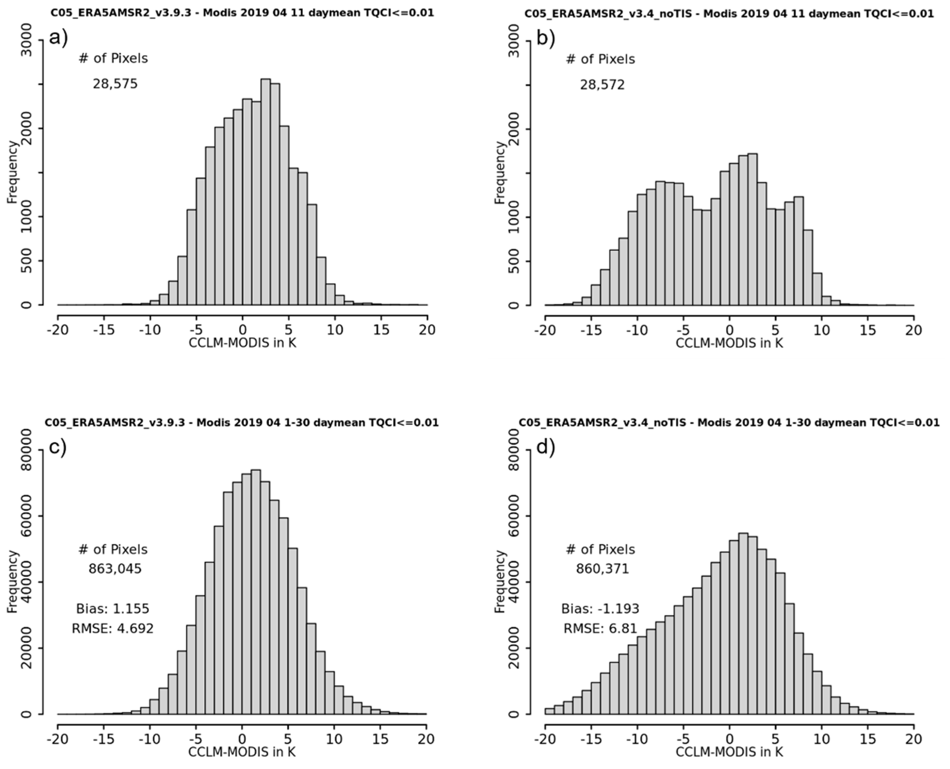
4.2. Comparison with MODIS Data

The comparison with MODIS IST data allows for a comparison for larger areas. CCLM surface temperatures are averaged daily to compare with the daily MODIS composites. However, there can be biases because of the sampling of the IST data, which are not evenly distributed over a day for a given pixel. MODIS data are resampled to the CCLM grid. As clouds affect the surface temperature both in the MODIS data and in CCLM, cloud filters were applied to both data sets. For MODIS, the vigorous Fuzzy Cloud Artefact Filter (FCAF) was applied [20]. For CCLM, values were discarded if the sum of integrated cloud liquid water and cloud ice exceeded 0.01 kg/m2. Figure 8a shows the frequency distribution of the difference between the surface temperature of CCLM and MODIS for 11 April 2019, when relatively low cloud coverage was present in the CCLM domain (more than 28,000 grid points are available for comparison). In general, CCLM and MODIS IST agree within ±4 K, in some cases the differences are up to ±10 K (Figure 8a). The frequency distribution for the old version (Figure 8b) on 11 April 2019 shows a second peak at the cold side of the distribution with much larger values for the underestimation of the surface temperature. These results are similar for the whole of April (Figure 8c). The overall bias for April 2019 is 1.2 K with an RMSE of 4.7 K (Figure 8c). Considering the error of about 2 K for the MODIS IST [21], this represents a very good agreement. For the old version of CCLM (Figure 8d), an underestimation of the IST by CCLM is found resulting in a considerable number of values exceeding −10 K difference.

5. Verification for the Vertical Structure of the Troposphere

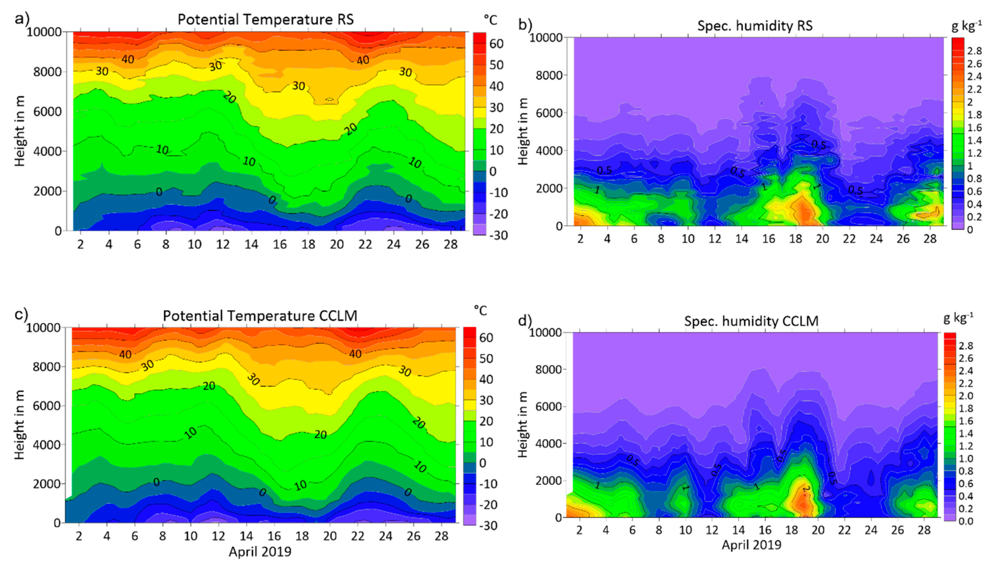
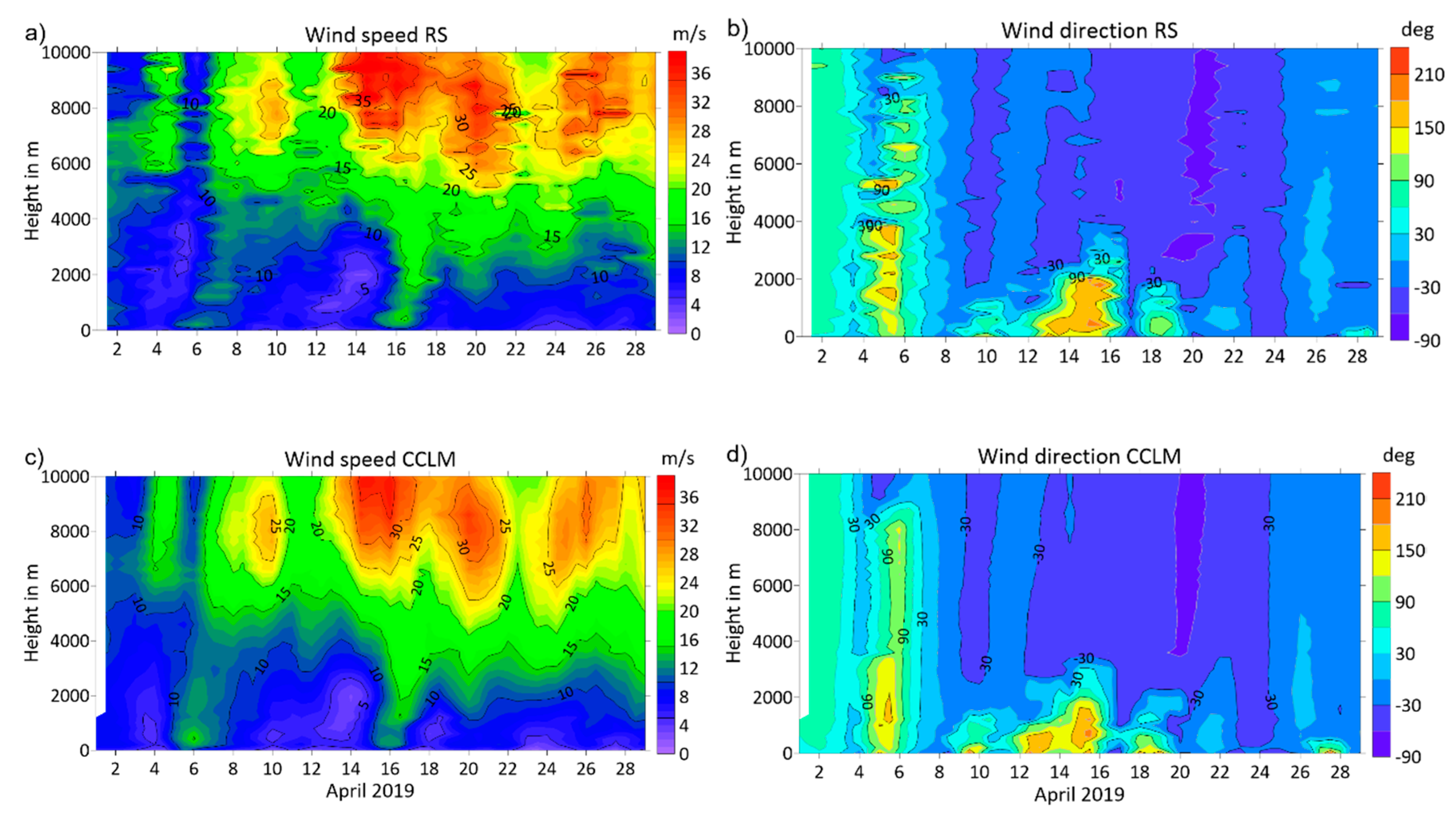
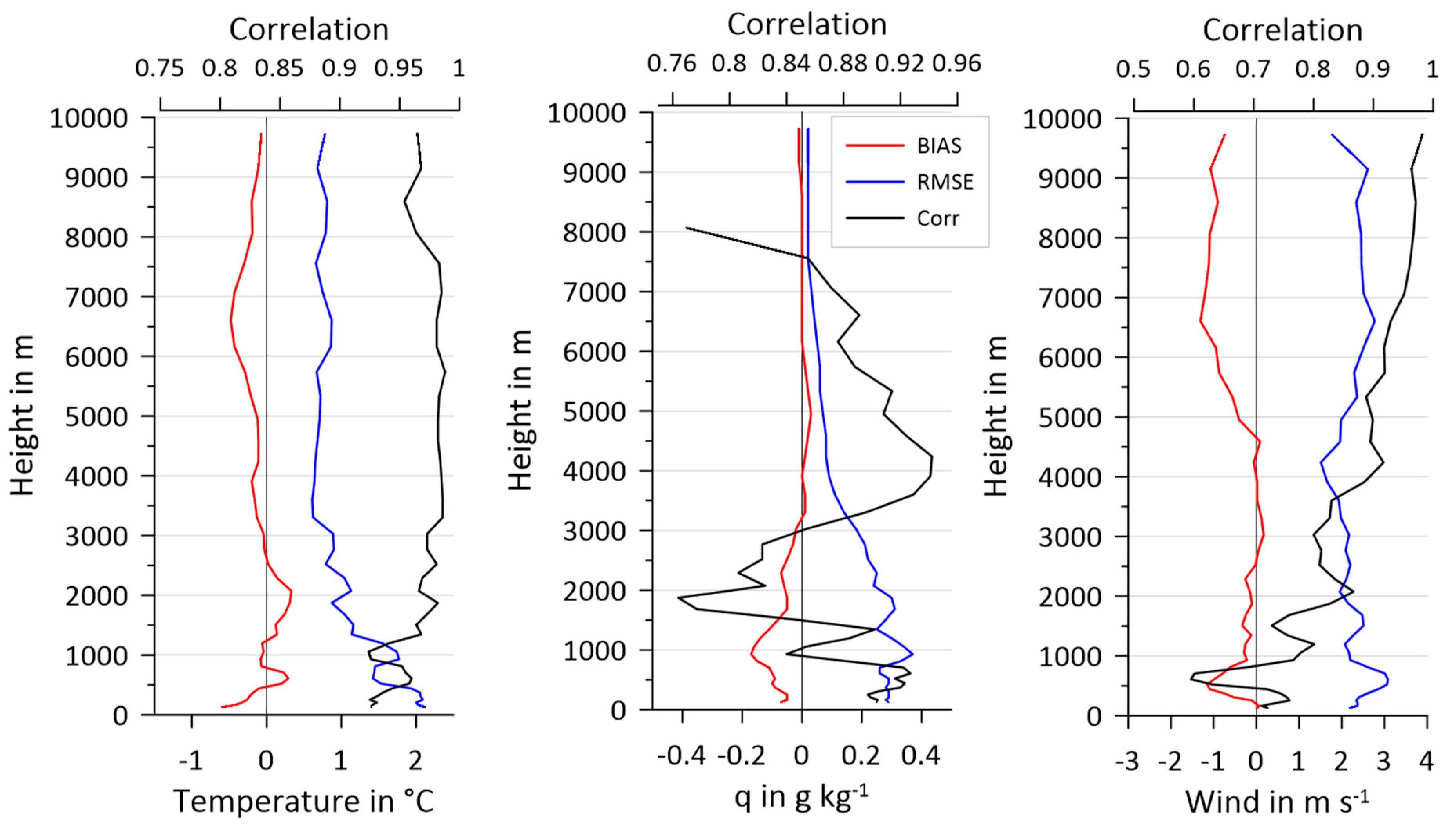
5.1. Verification Using Radiosondes

Although model and radiosonde data capture the lower part of the stratosphere, we restrict to the lowest 10 km. CCLM profiles were used at the time of the radiosonde launches, i.e., at 11:00 and 23:00 UTC (corresponding to simulation times of 17 and 29 h, respectively). Both data sets were interpolated to the same grid and using the same interpolation method. The results are shown for the potential temperature and specific humidity as time–height cross-sections for 1–29 April 2019 in Figure 9. Apart from the fact that the model fields are smoother than the measured ones, a remarkably good agreement is found. At the end of April, the radiosonde data show higher humidity values in the lowest 1000 m. For the wind speed and direction (Figure 10), the observed fields show more fluctuations than for temperature, but again very good agreement can be seen for the simulated fields. The upper-level jets are at the same height and have the same speed. A small difference can be seen for the low-level jet on 6 April, which is more pronounced in the simulations. An interesting feature can be seen for the period 18–20 April, where a distinct warming occurs throughout the troposphere and unusual high humidity values are observed in the lowest 2 km. Winds are easterly for low levels and veer to northerly and northwesterly directions above 2 km. During this period, a frontal system passed over the ship, which caused strong moisture advection (see Figure 3 and Figure 5).
The overall statistics of the comparisons with the radiosonde profile are presented in Figure 11. For this comparison, data on each model level were linearly detrended for the calculation of correlations. Radiosonde data were interpolated to the model levels. The first radiosonde level started usually at 150 m, so the lowest level for the comparison was 160 m (the eighth level of CCLM above the ground).
Temperature shows very small biases of less than ±0.5 K for almost all levels, the RMSE is 1.5–2.0 K in the lowest 1000 m and less than 1.0 K for the rest of the troposphere. The correlation is very high for all levels (r = 0.93–0.99). The biases for wind speed are also extremely small, while the RMSE has values of 2–3 m/s. The correlation is medium in the lowest 3000 m (r = 0.59–0.86) and increases for higher levels (r > 0.92 above 6000 m). For specific humidity, biases and RMSE are also very small; the correlation is high below 1500 m (r = 0.84–0.93), where most of the water vapor mass is present (see Figure 9). The decrease in the correlation above 7000 m is in regions where the humidity is extremely low.

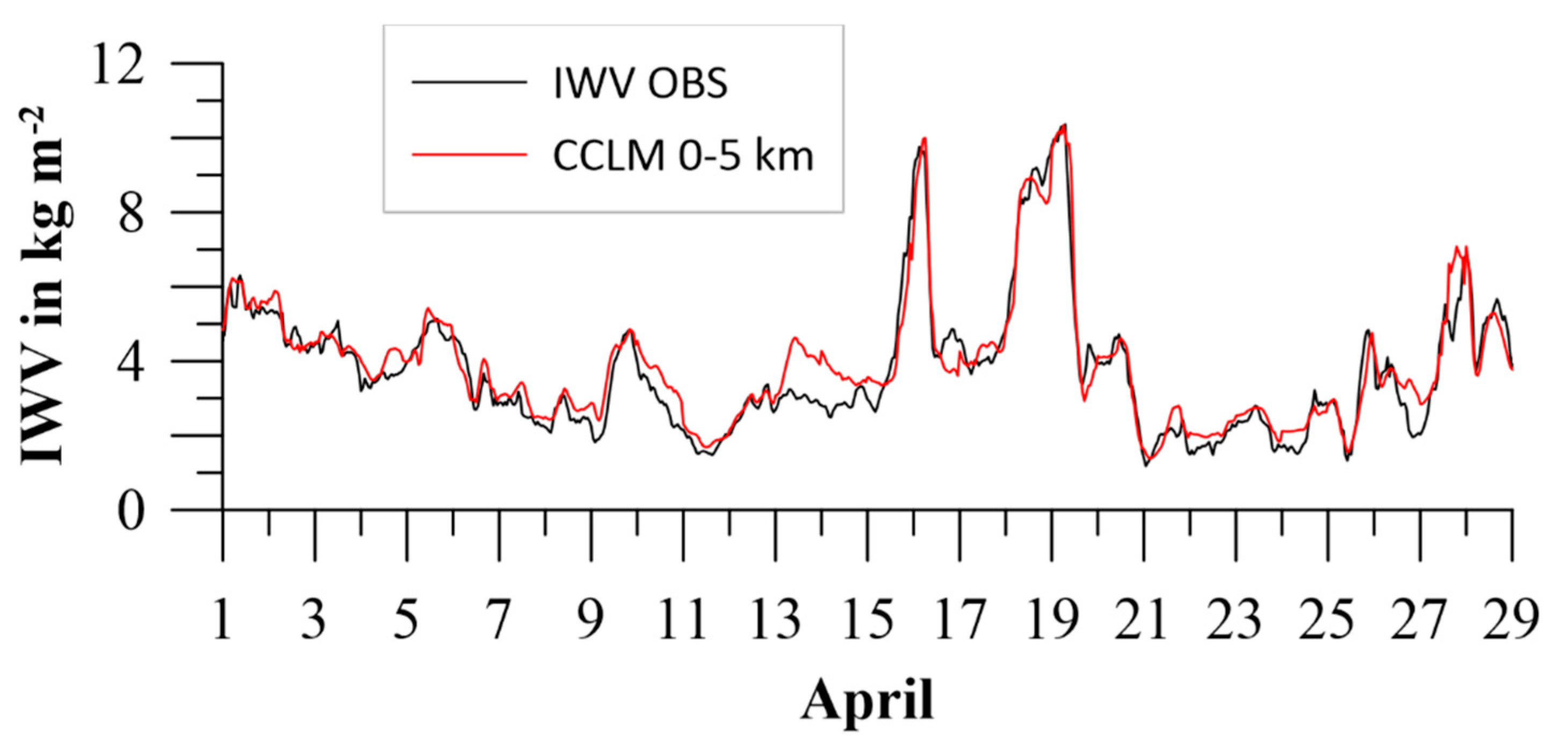
5.2. Verification Using Remote Sensing Integrated Water Vapor Data

In contrast to the twice-daily radiosondes, remote sensing instruments can probe the atmosphere at a much higher temporal resolution. The integrated water vapor (IWV) sensor onboard the ship (water vapor radiometer WVR) yielded IVW values for the lowest 5 km every hour. Figure 12 shows these observations together with the CCLM simulations (also for the lowest 5 km). The simulations agree very well with the observations. The bias (CCLM-OBS) is only 0.18 kg/m2, and standard deviations are almost identical (CCLM/OBS: 1.68/1.75). The high humidity event between 18 and 20 April, as discussed above, is also obvious in the IWV data, but a second event on 16 April can also be seen, which is not captured by the twice-daily radiosondes.

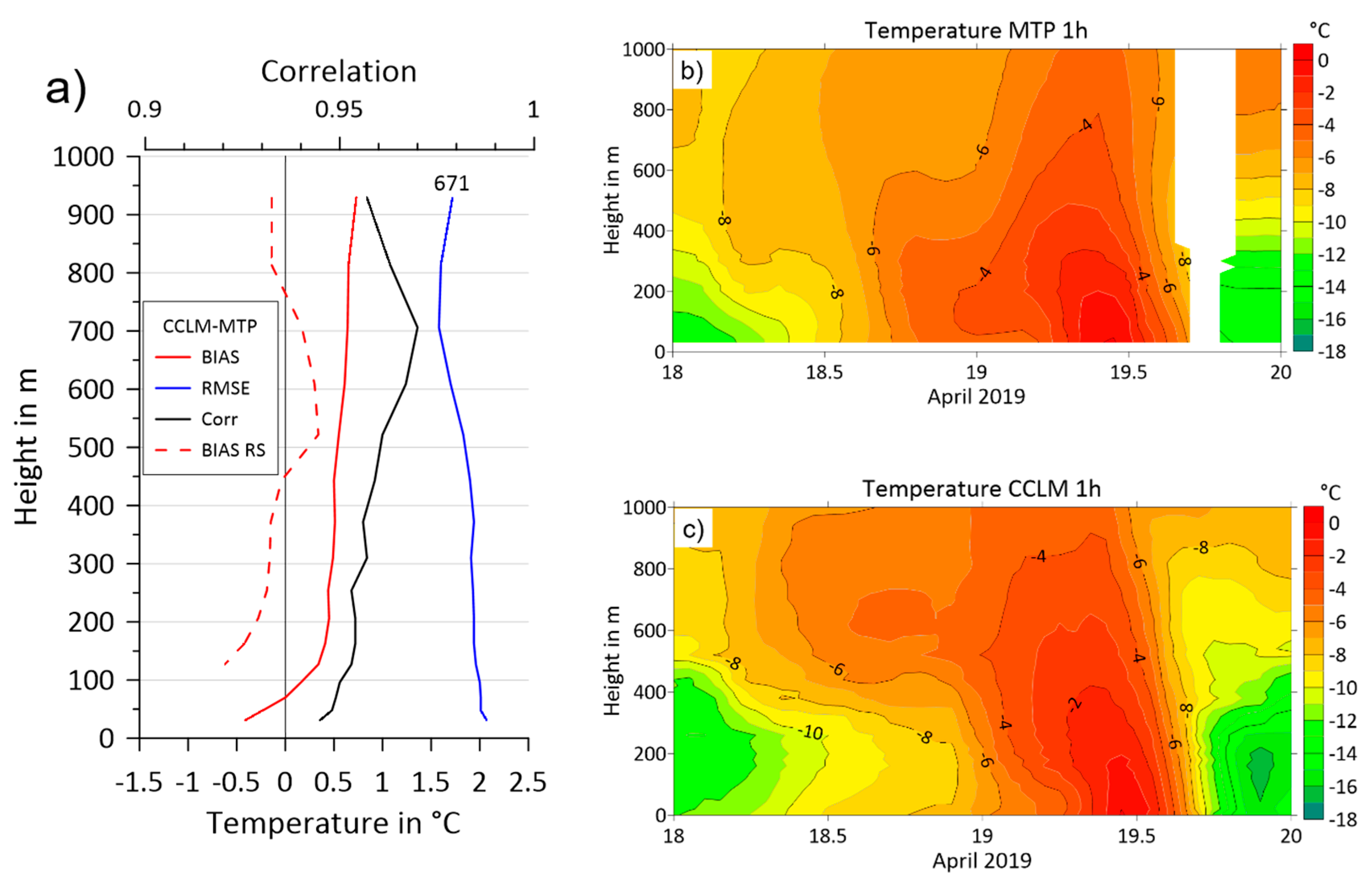
5.3. Verification Using Remote Sensing Temperature Profiler Data

The temperature profiler data (MTP5) were compared to the radiosondes by [15] and showed a good agreement. Here we use the same data covering the lowest 1000 m with a high temporal resolution of 1 h for the comparison with the 1-hourly CCLM data (Figure 13). MTP5 data were interpolated to the model levels. The first MTP5 level is at 30 m above sea level. The error of the MTP5 data is specified as 0.25–0.50 K for the lowest 300 m and 0.70–1.20 K between 400 and 1000 m [15].
While the bias (CCLM-MTP) is slightly negative for the lowest 50 m, it is around +0.5 K for all levels above 100 m. The comparison of the bias to the bias of CCLM with respect to radiosondes shows slightly lower values in the lowest 1000 m. The RMSE is 1.5–2.0 K, which is the same as for the radiosonde comparison. The correlation is very high and exceeds 0.95 at all levels.
The 1-hourly data allow a more detailed study for the warming period with unusual high humidity values during the period 18–20 April. As for the radiosondes, CCLM and MTP5 data were interpolated with the same method on the same grid for the cross-sections shown in Figure 13b,c. Both data sets show the warm front approaching at the end of 18 April and the maximum warming in the lowest 400 m in the first half of 19 April. In the second half of 19 April, strong cooling occurs with a maximum in the lowest 400 m, which is associated with a shift of the wind direction simulated by CCLM from southerly to northwesterly directions (not shown). Unfortunately, the MTP5 data show a gap for this cooling period. Overall, also the comparison of CCLM with MTP5 data at 1-hourly resolution shows a good quality of the simulations for the lowest 1000 m.

6. Discussion

Regional climate models (RCMs) are a valuable tool for improving our understanding of processes and interactions of the Arctic climate system. However, only few verification data sets on sea ice for the inner Arctic during winter are available, when atmosphere–ocean interactions are most pronounced and have strong impacts on the atmospheric boundary layer (ABL). On the other hand, the strongest stable boundary layers (SBL) also occur during winter over inland ice and sea ice.
The SHEBA campaign (1997–1998, [37]) was one of the few studies during winter which was intensively used for model verification [38]. Since icebreakers are needed in the inner Arctic during winter, most wintertime studies have focused on the marginal ice zone [6]. For the same reason, many experimental ship-based campaigns have been performed during summer, e.g., [39,40]. Ref. [11] used measurements onboard the well-instrumented icebreaker Oden for the verification of six RCMs (including CCLM) during summer 2014 with a focus on energy fluxes and tropospheric structure. Ref. [41] used the same set of models for a comparison with measurements of the Japanese ice-strengthened RV Mirai over the ice-free Arctic ocean during September 2014 with a focus on clouds and radiation. While CCLM was one of the few models that simulated low-level clouds correctly, the overall cloud amount was generally underestimated. This results in an underestimation of the downward longwave radiation and a large positive bias (100 W/m2) for the downward shortwave radiation. These findings cannot be confirmed by the present study. Although we find a slight underestimation of the downward longwave radiation, the bias in downward shortwave radiation is small.
The representation of sea ice in RCMs is of large importance for the simulation of near-surface quantities, particularly during winter. Most uncoupled RCMs use a rather simple description of sea ice, taking sea ice concentration (SIC) from the forcing data (reanalysis or GCM) with coarse resolution and assuming a fixed ice thickness for the grid-scale ice [11]. Using a tile approach [42] with flux averaging according to SIC is standard in all RCMs, but generally the non-ice fraction is assumed as open water. While this is true during summertime conditions, strong sea ice formation occurs in leads and polynyas during winter and open water areas are rare [19,43]. Even a few centimeters of thin ice have a strong effect on the heat fluxes during winter [13,24]. Thus, the representations of the sea ice distribution, the physical properties and the sub-grid thin ice are important.
On the other hand, the parameterizations of ice–atmosphere interactions are also important. Ref. [27] and [28] show that the modification of the turbulence scheme in CCLM for the SBL yielded a better representation of the near-surface temperature and the SBL structure over polar ice sheets. Over sea ice, these modifications resulted in an increased negative bias [27]. The present study confirms this finding, since a large negative bias is found for the old version of the sea-ice parameterizations, while the new version fits very well with the measurements taken during Transarktika 2019. In order to better understand the changes, Figure 14 shows the sea ice conditions as used by CCLM. Sea ice concentration in the CCLM grid point is larger than 90% most of the time. The grid-scale ice thickness is around 1.7 m for the whole period. For the sub-grid thin ice thickness, namely the thin ice thickness for leads, the values computed by CCLM range between 0 (open water) and 4 cm.
The largest differences between the old and new versions occur for the surface temperature for values below −20 °C. Figure 15 shows the dependence of the surface temperature (T0) simulated by CCLM on the simulated longwave downward radiation (Ld). Both quantities are well correlated, and a drop to very low temperatures can be seen for Ld smaller than 160 W/m2. This cooling occurs, when the available radiative energy defined as the net shortwave radiation plus Ld (Qdn = K * + Ld) also get very small (color code of the dots). This means that for clear sky situations during nighttime the snow layer in the old version cools too much. In the new version, the snow layer is thicker (Figure 14) and the snow-ice temperature can adapt to the heat flux from the ice into the snow layer, while snow-ice temperature stays constant in the old version.
The comparison with IST data from satellites is sensitive to artifacts caused by clouds, both in the model and the satellite data. On the other hand, it allows for a comparison for larger areas and a large number of grid points. Cloud effects are reduced by applying cloud filters both to MODIS and CCLM data. The resulting data yield more than 800,000 comparison points for April 2019. The absolute value of the bias of CCLM is comparable to the value for the 2 m temperature (although slightly positive, while being slightly negative for the 2 m temperature). The RMSE between CCLM and MODIS IST is much larger than for the 2 m temperature (4.7 K and 2.5 K, respectively). One reason for these differences can be that CCLM uses AMSR2 data for SIC, which results in different distributions of sea ice compared to MODIS. An underestimation of leads in AMSR SIC would be responsible for CCLM-MODIS being negative. A positive difference could result from the sampling of MODIS. While CCLM data represent a true daily average, MODIS overpasses have a gap around noon and possibly miss the warmest temperatures of the day.
The comparison of CCLM with radiosondes during Transarktika 2019 yields excellent results for the whole troposphere. The representation of the wind, temperature and moisture structure is very good. The comparison of the Transarktika 2019 results to the results for the summer campaign of [11] shows a similar good performance of CCLM for the temperature profiles, but better performance for the humidity profiles. The RMSE for the wind profiles is relatively large compared to the bias, but in the range of other studies with comparisons of simulations with radiosondes [27,44]. The evaluation of profiles from ERA5 data at the position of the ship in comparison with the radiosondes (not shown) yields a warm bias for the lowest 300 m, which is consistent with the warm bias of the 2m temperature. For the free atmosphere, the statistics for temperature are almost the same for ERA5 and CCLM. For the wind profile, ERA5 is similar to CCLM for the bias, but has a smaller RMSE and larger correlations. A better performance of ERA5 for the free atmosphere can be expected, since the radiosonde data of RV Akademik Tryoshnikov were submitted to the GTS and were likely used in the ERA5 reanalysis. Considering that CCLM data for the radiosonde comparison were taken for simulation times of 17 and 29 h, the performance of CCLM is very good.
The Transarktika 2019 campaign allows for comparisons of remote sensing data of IWV and the temperature profile for the lowest 1km with high temporal resolution. CCLM simulations show also excellent agreement with these measurements. The detailed study of a warming event during the period 18–20 April 2019 shows that this is caused by a short period of warm advection with southerly winds associated with a warm front. The inspection of the large-scale fields of CCLM show that the unusual high humidity during this warming event is related to the narrow warm sector of a frontal system, but not to an atmospheric river event [45].

7. Conclusions

Measurements of the tropospheric structure and near-surface variables during late winter of the inner Arctic have been performed during Transarktika 2019 in April 2019. The state-of-the-art RCM CCLM was evaluated using these data. Additionally, remote sensing data in the form of MODIS-derived IST were used. The main conclusions from this study are:
MODIS data represent a valuable data source for the verification of numerical models with respect to sea ice parameterization. A filtering of cloud artifacts is necessary.
The simulations using a new set of sea-ice parameterizations in CCLM show an excellent agreement with the measurements for the near-surface variables.
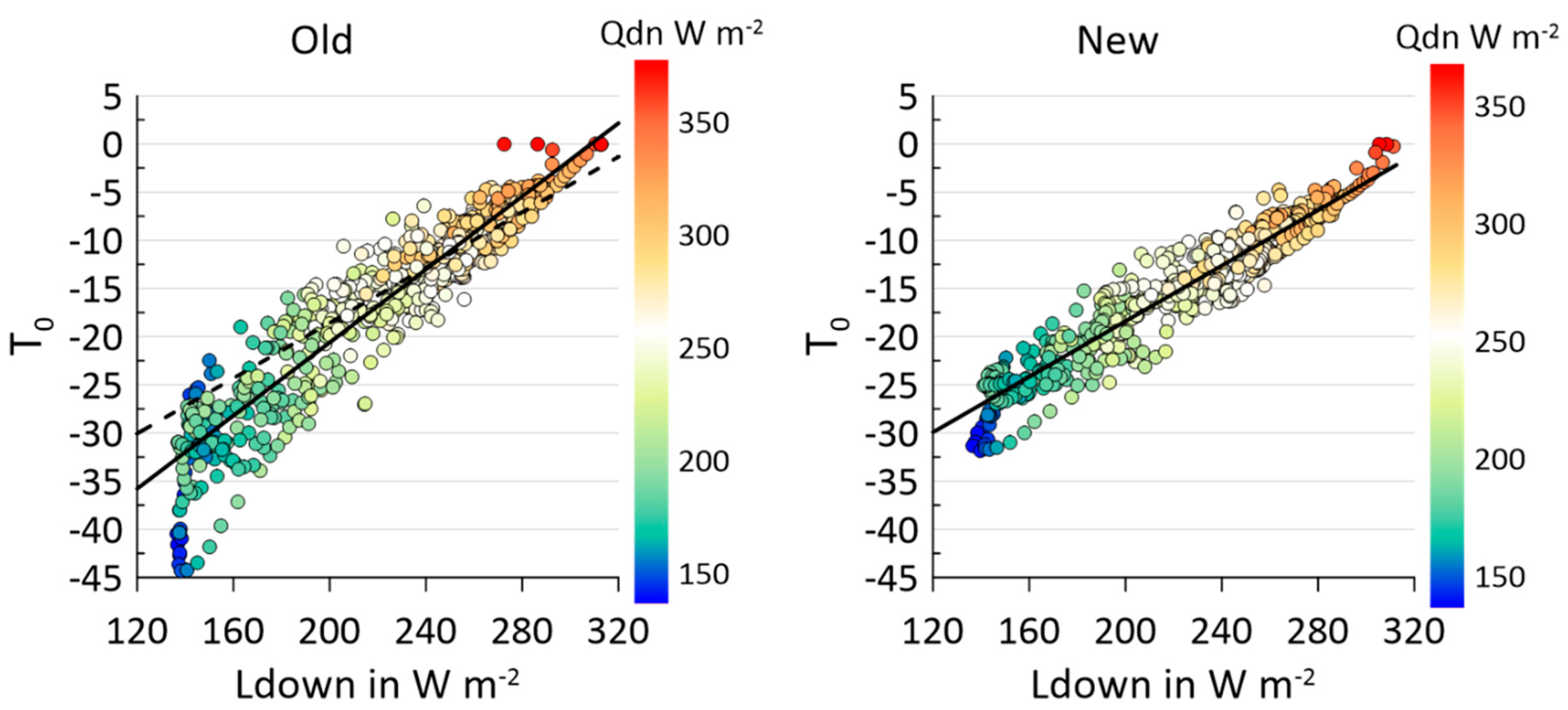
Radiation fluxes are represented well by CCLM, an underestimation is found for very low values of the downward longwave radiation.
The detailed study of a warming event during the period 18–20 April 2019 shows that this is caused by a short period of warm advection with southerly winds associated with a warm front. The inspection of the large-scale fields of CCLM shows that the unusual high humidity during this warming event is related to the narrow warm sector of a frontal system, but not to an atmospheric river event.
Overall, the data of Transarktika 2019 represent a valuable data set for the inner Arctic during late winter and should be used to check the representation of sea ice and the tropospheric structure in state-of-the-art RCMs, weather forecast models and in reanalyses.

Supplementary Materials

The following are available online at https://www.mdpi.com/2073-4433/12/2/174/s1, Figure S1: left: Bias (dots) and RMSE (squares) for the 2m-temperature (TC, values in K) and the 10m-wind. (FF10m, values in m/s) for different parameterizations (see text). Right: average daily 2m-temperature amplitude (in K) of observations and for different parameterizations., Table S1: Sea ice and parameterizations in CCLM as used in the “old” version [3] and in the present paper (“new”), Table S2: Tile approach parameterizations in CCLM as used in the “old” version [3] and in the present paper (“new”), Table S3: Boundary layer parameterizations in CCLM as used in the “old” version [3] with the adaption of the minimum diffusion coefficients and sub-grid TKE production of [16,17] (original values shown in brackets), and as used in the present paper (“new”).

Author Contributions

Conceptualization, G.H.; data curation, G.H., S.W., L.S., A.M., V.K. and I.M.; formal analysis, G.H. and S.W.; funding acquisition, G.H. and A.M.; methodology, G.H.; project administration, G.H.; supervision, G.H. and A.M.; visualization, G.H. and L.S.; writing—original draft, G.H.; writing—review and editing, G.H., S.W., L.S., A.M., V.K. and I.M. All authors have read and agreed to the published version of the manuscript.

Funding

This research was funded by the Federal Ministry of Education and Research (BMBF) under grant 03F0831C in the frame of German-Russian cooperation “WTZ RUS: Changing Arctic Transpolar System (CATS)” and the Russian Ministry of Education and Science (project RFMEFI61619 × 0108). The publication was funded by the Open Access Fund of the University of Trier and the German Research Foundation (DFG) within the Open Access Publishing funding program.

Institutional Review Board Statement

Not applicable.

Informed Consent Statement

Not applicable.

Data Availability Statement

The observational and model data will be made available on AARI data servers and PANGAEA. ERA5 data are available on the Copernicus Climate Change Service (C3S) Climate Data Store. https://cds.climate.copernicus.eu/#!/search?text=ERA5&type=dataset. MODIS data are available at https://nsidc.org/data/MOD29/versions/6 (accessed on 1 August 2020).

Acknowledgments

Thanks go to the CLM Community and the German Meteorological Service for providing the basic COSMO-CLM model. This work used resources of the Deutsches Klimarechenzentrum (DKRZ) granted by its Scientific Steering Committee (WLA) under project ID bb0474. We acknowledge the use of imagery from the NASA Worldview application (https://worldview.earthdata.nasa.gov), part of the NASA Earth Observing System Data and Information System (EOSDIS). We thank the NSIDC for providing the MODIS IST data. Model data processing was done with Climate Data Operators (CDO) (https://doi.org/10.5281/zenodo.3539275). Statistics were computed using the R software and the R package pracma.

Conflicts of Interest

The authors declare no conflict of interest.

References

  1. Hansen, J.; Ruedy, R.; Sato, M.; Lo, K. Global surface temperature change. Rev. Geophys. 2010, 48. [Google Scholar] [CrossRef] [Green Version]
  2. Serreze, M.C.; Stroeve, J. Arctic sea ice trends, variability and implications for seasonal ice forecasting. Philos. Trans. A Math. Phys. Eng. Sci. 2015, 373. [Google Scholar] [CrossRef] [Green Version]
  3. Stroeve, J.C.; Kattsov, V.; Barrett, A.; Serreze, M.; Pavlova, T.; Holland, M.; Meier, W.N. Trends in Arctic sea ice extent from CMIP5, CMIP3 and observations. Geophys. Res. Lett. 2012, 39. [Google Scholar] [CrossRef] [Green Version]
  4. Kohnemann, S.H.E.; Heinemann, G.; Bromwich, D.H.; Gutjahr, O. Extreme Warming in the Kara Sea and Barents Sea during the Winter Period 2000–16. J. Clim. 2017, 30, 8913–8927. [Google Scholar] [CrossRef]
  5. Lüpkes, C.; Vihma, T.; Birnbaum, G.; Wacker, U. Influence of leads in sea ice on the temperature of the atmospheric boundary layer during polar night. Geophys. Res. Lett. 2008, 35. [Google Scholar] [CrossRef] [Green Version]
  6. Cohen, L.; Hudson, S.R.; Walden, V.P.; Graham, R.M.; Granskog, M.A. Meteorological conditions in a thinner Arctic sea ice regime from winter to summer during the Norwegian Young Sea Ice expedition (N-ICE2015). J. Geophys. Res. 2017, 122, 7235–7259. [Google Scholar] [CrossRef] [Green Version]
  7. DuVivier, A.K.; Cassano, J.J. Evaluation of WRF Model Resolution on Simulated Mesoscale Winds and Surface Fluxes near Greenland. Mon. Wea. Rev. 2013, 141, 941–963. [Google Scholar] [CrossRef]
  8. Gutjahr, O.; Heinemann, G. A model-based comparison of extreme winds in the Arctic and around Greenland. Int. J. Climatol. 2018, 38, 5272–5292. [Google Scholar] [CrossRef] [Green Version]
  9. Dee, D.P.; Uppala, S.M.; Simmons, A.J.; Berrisford, P.; Poli, P.; Kobayashi, S.; Andrae, U.; Balmaseda, M.A.; Balsamo, G.; Bauer, P.; et al. The ERA-Interim reanalysis: Configuration and performance of the data assimilation system. Q. J. R. Meteorol. Soc. 2011, 137, 553–597. [Google Scholar] [CrossRef]
  10. Akperov, M.; Rinke, A.; Mokhov, I.I.; Matthes, H.; Semenov, V.A.; Adakudlu, M.; Cassano, J.; Christensen, J.H.; Dembitskaya, M.A.; Dethloff, K.; et al. Cyclone Activity in the Arctic From an Ensemble of Regional Climate Models (Arctic CORDEX). J. Geophys. Res. 2018, 123, 2537–2554. [Google Scholar] [CrossRef]
  11. Sedlar, J.; Tjernström, M.; Rinke, A.; Orr, A.; Cassano, J.; Fettweis, X.; Heinemann, G.; Seefeldt, M.; Solomon, A.; Matthes, H.; et al. Confronting Arctic troposphere, clouds, and surface energy budget representations in regional climate models with observations. J. Geophys. Res. 2020, 125, e2019JD031783. [Google Scholar] [CrossRef]
  12. Preußer, A.; Ohshima, K.I.; Iwamoto, K.; Willmes, S.; Heinemann, G. Retrieval of Wintertime Sea Ice Production in Arctic Polynyas Using Thermal Infrared and Passive Microwave Remote Sensing Data. J. Geophys. Res. Oceans 2019, 124, 5503–5528. [Google Scholar] [CrossRef] [Green Version]
  13. Gutjahr, O.; Heinemann, G.; Preußer, A.; Willmes, S.; Drüe, C. Quantification of ice production in Laptev Sea polynyas and its sensitivity to thin-ice parameterizations in a regional climate model. Cryosphere 2016, 10, 2999–3019. [Google Scholar] [CrossRef] [Green Version]
  14. Frolov, I.E.; Ivanov, V.V.; Filchuk, K.V.; Makshtas, A.P.; Kustov, V.Y.; Mahotina, I.A.; Ivanov, B.V.; Urazgildeeva, A.V.; Syoemin, V.L.; Zimina, O.L.; et al. Transarktika-2019: Winter expedition in the Arctic Ocean on the R/V “Akademik Tryoshnikov”. Probl. Arktiki Antarkt. 2019, 65, 255–274. [Google Scholar] [CrossRef] [Green Version]
  15. Makshtas, A.P.; Il’in, G.N.; Bykov, V.Y.; Miller, E.A.; Troitsky, A.V.; Kustov, V.Y.; Bolshakova, I.I.; Rize, D.D. The experience of remote temperature-water content sounding of atmosphere during drift of R/V “Akademik Tryoshnikov”. Probl. Arktiki Antarkt. 2020, 66, 349–363. [Google Scholar] [CrossRef]
  16. Spreen, G.; Kaleschke, L.; Heygster, G. Sea ice remote sensing using AMSR-E 89-GHz channels. J. Geophys. Res. 2008, 113. [Google Scholar] [CrossRef] [Green Version]
  17. Huntemann, M.; Heygster, G.; Kaleschke, L.; Krumpen, T.; Mäkynen, M.; Drusch, M. Empirical sea ice thickness retrieval during the freeze-up period from SMOS high incident angle observations. Cryosphere 2014, 8, 439–451. [Google Scholar] [CrossRef] [Green Version]
  18. Hall, D.K.; Riggs, G.A. MODIS/Terra Sea Ice Extent 5-Min L2 Swath 1km, Version 6 [Northern Hemisphere]; NASA National Snow and Ice Data Center Distributed Active Archive Center: Boulder, CO, USA, 2015. [Google Scholar] [CrossRef]
  19. Preußer, A.; Heinemann, G.; Willmes, S.; Paul, S. Circumpolar polynya regions and ice production in the Arctic: Results from MODIS thermal infrared imagery from 2002/2003 to 2014/2015 with a regional focus on the Laptev Sea. Cryosphere 2016, 10, 3021–3042. [Google Scholar] [CrossRef] [Green Version]
  20. Reiser, F.; Willmes, S.; Heinemann, G. A New Algorithm for Daily Sea Ice Lead Identification in the Arctic and Antarctic Winter from Thermal-Infrared Satellite Imagery. Remote Sens. 2020, 12, 1957. [Google Scholar] [CrossRef]
  21. Hall, D.K.; Key, J.R.; Case, K.A.; Riggs, G.A.; Cavalieri, D.J. Sea ice surface temperature product from MODIS. IEEE Trans. Geosci. Remote Sens. 2004, 42, 1076–1087. [Google Scholar] [CrossRef]
  22. Willmes, S.; Heinemann, G. Sea-Ice Wintertime Lead Frequencies and Regional Characteristics in the Arctic, 2003–2015. Remote Sens. 2016, 8, 4. [Google Scholar] [CrossRef] [Green Version]
  23. Rockel, B.; Will, A.; Hense, A. The Regional Climate Model COSMO-CLM (CCLM). Meteorol. Z. 2008, 17, 347–348. [Google Scholar] [CrossRef]
  24. Bauer, M.; Schröder, D.; Heinemann, G.; Willmes, S.; Ebner, L. Quantifying polynya ice production in the Laptev Sea with the COSMO model. Polar Res. 2013, 32, 20922. [Google Scholar] [CrossRef]
  25. Ebner, L.; Schröder, D.; Heinemann, G. Impact of Laptev Sea flaw polynyas on the atmospheric boundary layer and ice production using idealized mesoscale simulations. Polar Res. 2011, 30, 7210. [Google Scholar] [CrossRef]
  26. Platonov, V.; Kislov, A. High-Resolution COSMO-CLM Modeling and an Assessment of Mesoscale Features Caused by Coastal Parameters at Near-Shore Arctic Zones (Kara Sea). Atmosphere 2020, 11, 1062. [Google Scholar] [CrossRef]
  27. Zentek, R.; Heinemann, G. Verification of the regional atmospheric model CCLM v5.0 with conventional data and lidar measurements in Antarctica. Geosci. Model. Dev. 2020, 13, 1809–1825. [Google Scholar] [CrossRef] [Green Version]
  28. Heinemann, G. Assessment of Regional Climate Model Simulations of the Katabatic Boundary Layer Structure over Greenland. Atmosphere 2020, 11, 571. [Google Scholar] [CrossRef]
  29. Hersbach, H.; Bell, B.; Berrisford, P.; Hirahara, S.; Horányi, A.; Muñoz-Sabater, J.; Nicolas, J.; Peubey, C.; Radu, R.; Schepers, D.; et al. The ERA5 global reanalysis. Q. J. R. Meteorol. Soc. 2020, 146, 1999–2049. [Google Scholar] [CrossRef]
  30. Hersbach, H.; de Rosnay, P.; Bell, B.; Schepers, D.; Simmons, A.; Soci, C.; Abdalla, S.; Alonso-Balmaseda, M.; Balsamo, G.; Bechtold, P.; et al. Operational Global Reanalysis: Progress, Future Directions and Synergies with NWP; European Centre for Medium Range Weather Forecasts: Reading, UK, 2018. [Google Scholar] [CrossRef]
  31. Zhang, J.; Rothrock, D.A. Modeling Global Sea Ice with a Thickness and Enthalpy Distribution Model in Generalized Curvilinear Coordinates. Mon. Weather. Rev. 2003, 131, 845–861. [Google Scholar] [CrossRef]
  32. Hastings, D.A.; Dunbar, P.K. Global Land One-kilometer Base Elevation (GLOBE) Digital Elevation Model, Documentation. Key Geophys. Rec. Doc. (KGRD) 1999, 1–147. [Google Scholar]
  33. Zentek, R. COSMO Documentation (Archived Version from 2019, Uploaded with Permission of the DWD). 2019. Available online: https://zenodo.org/record/3339384 (accessed on 13 May 2020).
  34. Schröder, D.; Heinemann, G.; Willmes, S. The impact of a thermodynamic sea-ice module in the COSMO numerical weather prediction model on simulations for the Laptev Sea, Siberian Arctic. Polar Res. 2011, 30, 6334. [Google Scholar] [CrossRef]
  35. Doms, G.; Förstner, J.; Heise, H.; Herzog, H.-J.; Mironov, D.; Raschendorfer, M.; Reinhardt, T.; Ritter, B.; Schrodin, R.; Schulz, J.-P.; et al. A Description of the Nonhydrostatic Regional COSMO-Model. Part. II. Physical Parameterizations; Offenbach: Cologne, Germany, 2013. [Google Scholar]
  36. Ritter, B.; Geleyn, J.-F. A Comprehensive Radiation Scheme for Numerical Weather Prediction Models with Potential Applications in Climate Simulations. Mon. Weather. Rev. 1992, 120, 303–325. [Google Scholar] [CrossRef] [Green Version]
  37. Uttal, T.; Curry, J.A.; Mcphee, M.G.; Perovich, D.K.; Moritz, R.E.; Maslanik, J.A.; Guest, P.S.; Stern, H.L.; Moore, J.A.; Turenne, R.; et al. Surface Heat Budget of the Arctic Ocean. Bull. Amer. Meteor. Soc. 2002, 83, 255–275. [Google Scholar] [CrossRef] [Green Version]
  38. Rinke, A.; Dethloff, K.; Cassano, J.J.; Christensen, J.H.; Curry, J.A.; Du, P.; Girard, E.; Haugen, J.-E.; Jacob, D.; Jones, C.G.; et al. Evaluation of an ensemble of Arctic regional climate models: Spatiotemporal fields during the SHEBA year. Clim. Dyn. 2006, 26, 459–472. [Google Scholar] [CrossRef]
  39. Sotiropoulou, G.; Tjernström, M.; Sedlar, J.; Achtert, P.; Brooks, B.J.; Brooks, I.M.; Persson, P.O.G.; Prytherch, J.; Salisbury, D.J.; Shupe, M.D.; et al. Atmospheric Conditions during the Arctic Clouds in Summer Experiment (ACSE): Contrasting Open Water and Sea Ice Surfaces during Melt and Freeze-Up Seasons. J. Clim. 2016, 29, 8721–8744. [Google Scholar] [CrossRef] [Green Version]
  40. Tjernström, M.; Leck, C.; Persson, P.O.G.; Jensen, M.L.; Oncley, S.P.; Targino, A. The Summertime Arctic Atmosphere: Meteorological Measurements during the Arctic Ocean Experiment 2001. Bull. Am. Meteorol. Soc. 2004, 85, 1305–1322. [Google Scholar] [CrossRef]
  41. Inoue, J.; Sato, K.; Rinke, A.; Cassano, J.J.; Fettweis, X.; Heinemann, G.; Matthes, H.; Orr, A.; Phillips, T.; Seefeldt, M.; et al. Clouds and radiation processes in regional climate models evaluated using observations over the ice-free Arctic Ocean. J. Geophys. Res. 2020. [Google Scholar] [CrossRef]
  42. Heinemann, G.; Kerschgens, M. Simulation of surface energy fluxes using high-resolution non-hydrostatic simulations and comparisons with measurements for the LITFASS-2003 experiment. Bound-Layer Meteorol. 2006, 121, 195–220. [Google Scholar] [CrossRef]
  43. Willmes, S.; Krumpen, T.; Adams, S.; Rabenstein, L.; Haas, C.; Hoelemann, J.; Hendricks, S.; Heinemann, G. Cross-validation of polynya monitoring methods from multisensor satellite and airborne data: A case study for the Laptev Sea. Can. J. Remote Sens. 2010, 36, S196–S210. [Google Scholar] [CrossRef]
  44. Souverijns, N.; Gossart, A.; Demuzere, M.; Lenaerts, J.T.M.; Medley, B.; Gorodetskaya, I.V.; Vanden Broucke, S.; van Lipzig, N.P.M. A New Regional Climate Model for POLAR-CORDEX: Evaluation of a 30-Year Hindcast with COSMO-CLM 2 over Antarctica. J. Geophys. Res. 2019, 124, 1405–1427. [Google Scholar] [CrossRef] [Green Version]
  45. Gorodetskaya, I.V.; Tsukernik, M.; Claes, K.; Ralph, M.F.; Neff, W.D.; van Lipzig, N.P.M. The role of atmospheric rivers in anomalous snow accumulation in East Antarctica. Geophys. Res. Lett. 2014, 41, 6199–6206. [Google Scholar] [CrossRef] [Green Version]
Figure 1. Left: Model domain of the COSMO-CLM (CCLM) model with 5 km resolution with topography and sea ice concentration for 15 April 2019 and ship positions for 5, 12, 19 and 25 April 2019. Right: subsection of the model domain with daily ship positions during the drift (numbers are the days of April) and sea ice conditions for 15 April 2019. In addition to sea ice concentration, thin-ice thickness (TIT) from Soil Moisture and Ocean Salinity (SMOS) data are shown.
Atmosphere 12 00174 g001
Figure 2. (a) Photo of the meteorological tower with “R/V Akademik Tryoshnikov” in the background (photo: V. Kustov). (b) Moderate Resolution Imaging Spectroradiometer (MODIS) image (visible channel, 250 m resolution) for 06:00 UTC 11 April 2019. The position of “R/V Akademik Tryoshnikov” is indicated by a circle (image from NASA worldview).
Atmosphere 12 00174 g002
Figure 3. Pressure and 2 m temperature (upper panels), and 10 m wind speed and direction (lower panels) for the period 1 to 29 April 2019 for the observations (1 h values (3 h values for wind direction), black) and CCLM simulations (1 h values, red). For 2 m temperature, ERA5 data are shown as a blue line.
Atmosphere 12 00174 g003
Figure 4. As in Figure 3, but for downward shortwave (Kd) and downward longwave radiation (Ld).
Atmosphere 12 00174 g004
Figure 5. Fields of CCLM-simulated MSLP, 10 m wind and 2 m temperature at 12:00 UTC for (a) 5, (b) 12, (c) 19 and (d) 25 April 2019. The ship position is marked with a white dot (see also Figure 1).
Atmosphere 12 00174 g005
Figure 6. Frequency distributions of measured and simulated values (1 h values) and their differences: (a) 2 m temperature, (b) 10 m wind speed, (c) pressure, (d) downward shortwave radiation, (e) downward longwave radiation, (f) net radiation.
Atmosphere 12 00174 g006
Figure 7. Frequency distributions of measured and simulated values (1 h values) and their differences: (a) 2 m temperature and (b) 10 m wind speed for the old version (Supplementary Tables S1–S3), and (c) 2 m temperature and (d) downward longwave radiation from ERA5 data.
Atmosphere 12 00174 g007
Figure 8. Frequency distributions of differences between the surface temperature over sea ice areas of CCLM and MODIS for (a/c) 11 April 2019/whole April 2019 for the new version, (b/d) 11 April 2019/whole April 2019 for the old version after cloud filtering (see text).
Atmosphere 12 00174 g008
Figure 9. Time–height cross-sections for the potential temperature from radiosondes (a) and CCLM (c) and for the specific humidity of the from radiosondes (b) and CCLM (d) for 1–29 April 2019.
Atmosphere 12 00174 g009
Figure 10. Time–height cross-sections for the wind speed from radiosondes (a) and CCLM (c) and for the wind direction from radiosondes (b) and CCLM (d) for 1–29 April 2019.
Atmosphere 12 00174 g010
Figure 11. Profiles of bias, RMSE and correlation for the comparison of CCLM with radiosondes for temperature (left), specific humidity (middle) and wind speed (right) for 1–29 April 2019 (54 profiles).
Atmosphere 12 00174 g011
Figure 12. Observations (black) and simulations (red) of the integrated water vapor (IWV) for April 2019.
Atmosphere 12 00174 g012
Figure 13. Comparisons of CCLM with 1h temperature data of the MTP5 profiler. (a) Profiles of bias, RMSE and correlation for 1–29 April 2019 (671 profiles), the profile of the bias CCLM compared to radiosondes is shown as a dashed line. Time–height cross-sections for the temperature for 18–20 April 2019 for CCLM (b) and (c) for the MTP5 profiler.
Atmosphere 12 00174 g013
Figure 14. Sea ice conditions as used by CCLM for the grid point of R/V “Akademik Tryoshnikov” with daily resolution for 1–29 April 2019. Lower panel: sea ice concentration (SIC, green) and ice thickness (blue). Upper panel: sub-grid scale thin ice thickness (lines without symbols, black/red: new/old parameterization.
Atmosphere 12 00174 g014
Figure 15. Scatter plots of the surface temperature against downward longwave radiation as simulated by CCLM for the old version (left) and the new version (right). The color code is the available radiative energy (Qdn = K * + Ld). Full lines are the regression of the respective data, the dashed line in the left panel is the regression of the new version.
Atmosphere 12 00174 g015
Table 1. Meteorological instrumentation during Transarktika in April 2019.
TowerHeightSensorInstrument TypeSamplingData Resolution
Temperature2 m, 8 mHMP155Vaisala1 min averaging1 h
Humidity2 m, 8 mHMP155Vaisala1 min averaging1 h
Wind2 m, 10 mPropeller, wind vaneRM Young 05108-451 min averaging1 h
Radiation 4 components2 mCNR4Kipp&Zonen1 min averaging1 h
Pressure1 mPTB110 Vaisala1 min averaging1 h
On ship
Ceilometer0–15 kmCL51Vaisala2 s1h
MTP5 temperature profiles0–1000 mMTP-5PEATTEX5 min averaging1 h, vertically variable (10–50 m)
Integrated water vapor 0–5 kmRVPIPA-RAS10 min1 h, vertically integrated
Radiosonde
PTU, wind
0.1–25 kmPolus-MRadiy1 sTwice-daily, vertically variable (standard and significant levels)
Table 2. Comparison of CCLM with near-surface observations (OBS) for April 2019 (2 m temperature (T), 10 m wind speed (wind), pressure (p), downward shortwave (Kd), downward longwave radiation (Ld) and net radiation (Q)). Average amplitude (AA) is the difference between the 90% and 10% percentiles (after subtraction of the low-pass filtered time series, see text). RMSE = root mean square error, Corr = correlation, number of values is 674.
QuantityOBSCCLMBiasRMSECorr.AADiff AA (CCLM-OBS)
T in °C−13.7−14.8−1.12.50.9278.3−0.6
Wind in m/s5.54.6−1.01.70.799
P in hPa1013.51013.90.40.90.996
Kd in W/m211112413340.94923213
Ld in W/m2233222−11300.797
Q in W/m2−3−13−10220.629510.5
Publisher’s Note: MDPI stays neutral with regard to jurisdictional claims in published maps and institutional affiliations.

