Article

Tropical Overshooting Cloud-Top Height Retrieval from Himawari-8 Imagery Based on Random Forest Model

1
Department of Atmospheric and Oceanic Sciences, School of Physics, Peking University, Beijing 100871, China
2
Department of Atmospheric and Oceanic Sciences, University of California, Los Angeles, CA 90095, USA
3
Shanghai Central Meteorological Observatory, Shanghai 200030, China
*
Author to whom correspondence should be addressed.
Atmosphere 2021, 12(2), 173; https://doi.org/10.3390/atmos12020173
Submission received: 21 December 2020 / Revised: 21 January 2021 / Accepted: 25 January 2021 / Published: 28 January 2021
(This article belongs to the Section Meteorology)

Abstract

:
Tropical overshooting convection has a strong impact on both heat budget and moisture distribution in the upper troposphere and lower stratosphere, and it can pose a great risk to aviation safety. Cloud-top height is one of the essential concerns of overshooting convection for both the climate system and the aviation weather forecast. The main purpose of our work is to verify the application of the machine learning method, taking the random forest (RF) model as an instance, in overshooting cloud-top height retrieval from Himawari-8 data. By using collocated CloudSat observations as a reference, we utilize several infrared indicators of Himawari-8 that are commonly recognized to relate to cloud-top height, along with some temporal and geographical parameters (latitude, month, satellite zenith angle, etc.), as predictors to construct and validate the model. Analysis of variable importance shows that the brightness temperature of 6.2 um acts as the dominant predictor, followed by satellite zenith angle, brightness temperature of 13.3 um, latitude, and month. In the comparison between the RF model and the traditional single-channel interpolation method, retrievals from the RF model agree well with observation with a high correlation coefficient (0.92), small RMSE (222 m), and small MAE (164 m), while these metrics from traditional single-channel interpolation method shows lower skills (0.70, 1305 m, and 1179 m). This work presents a new sight of overshooting cloud-top height retrieval based on the machine learning method.

1. Introduction

Overshooting convection, which is a small subset of clouds with strong convective updrafts that penetrate the upper troposphere–lower stratosphere (UTLS) region, has been widely recognized to be related to the transport of various atmospheric constituents and chemical species from the troposphere into the stratosphere. It plays an important role in moisture distribution and energy budgets globally [1,2,3,4,5], and the height of overshooting clouds indicates the altitude to which tropospheric air parcels are transported. The cloud-top height (CTH) of overshooting clouds is also required by aviation weather forecast since it is an indication of strong vertical development of deep convective cores [6] and convectively induced turbulence caused by gravity wave breaking [7] which occurs at ≈1 km above overshooting tops causing damage to flight [8]. Hence, the importance of accurately obtaining the CTH of overshooting clouds globally and at high frequency is underscored.
Methods of CTH retrieval from both ground- and satellite-based remote sensing data have been developed for several years. As for active sensors, reflectivity echo-top height Radar or Lidar (active sensors) could act as a reference of CTH directly, including Micro-Pulse Lidar (MPL) and millimeter wavelength cloud radar (MMCR) at the South Great Plain of USA [9], Ka-band Doppler cloud radar(Beijing, China) [10], the WSR-88D(NOAA, USA) [11], the Precipitation Radar onboard the Tropical Rainfall Measuring Mission (TRMM, NASA, USA) satellite [12,13], dual-frequency radar (DPR) on board of Global Precipitation Measurement (GMP, NASA, USA) satellite [14], the Cloud Profiling Radar (CPR) of the CloudSat Mission (Het Propulsion Laboratory, USA) [6,15], and Cloud-Aerosol Lidar with Orthogonal Polarization (CALIPSO, NASA, USA) [16], etc. The Multiangle Imaging Spectroradiometer (MISR) onboard Terra satellite could also use the camera to retrieve stereo CTH using a stereo-matching algorithm [17]. The ground-based instrument usually has a high spatial and temporal resolution, but its spatial and temporal coverages are very limited. Most active sensors onboard polar-orbiting satellites (e.g., CloudSat/CPR, MISR) could improve the spatial continuity, but their spatial coverage is limited to the narrow footprint, and their temporal frequency is limited by the circling period of polar-orbiting satellites. Even though DPR onboard GPM could provide a near-global view of 3D cloud and precipitation structure in 2–3 h, it is still hard to provide near-real-time CTH retrieval.
Geostationary satellites provide a way of monitoring the spatial distribution and temporal development of convective clouds by using atmospheric window and various gas-absorbing channel measurements. There are several well-developed methods widely used in CTH estimates [18], including the interpolation method which is based on the sole infrared window (IRW) channel (for opaque cloud), radiance ratio method (such as CO2-IRW ratio method, O3-CO2 ratio method, etc.), and the intercept method (for the semitransparent cloud). The CTH of high-resolution Cloud Analysis Information (HCAI) derived from Himawari-8 (HMW8) has been proposed by the Japan Meteorological Agency (JMA, Tokyo, Japan), but this product has been tested to significantly underestimate CTHs higher than 14.5 km. Even though they attribute this problem to undetectably thin and high cloud layers, it is significant that the higher the cloud the larger the underestimate [19]. A new method promoted based on a lapse rate determined by the overshooting-anvil brightness temperature and height differences significantly improves the accuracy of extreme overshooting cloud-top height retrieval [20]. However, most of these methods need the auxiliary of numerical weather prediction (NWP) model data. The stereoscopic method is also an accurate method for cloud-top height derivation, which uses the slanted views of joint satellites but can only be used for limited regions [21,22]. Besides, the length of shadow above the anvil using visible-channel imagery [23] could also be used to determine the magnitude of penetration, which can be transformed to the relative height between penetration and anvil cloud height. However, since the length of the shadow depends on the solar zenith angle and referenced the anvil cloud, the application of this method is subjective and limited to daylight.
Machine learning (ML) algorithms such as random forest (RF), support vector machines (SVM), and artificial neural networks, etc., have been successfully adapted to remote sensing and geoscience [19,24,25,26,27,28,29]. Previous research treated all kinds of cloud equally into training and testing datasets to test the application of the machine learning method on CTH retrieval [19,30], such as neural network, K-nearest-neighbor, support vector machine, gradient boosting decision tree, etc., and their results manifest the good performance in CTH assignment. However, some machine-learning-based models show underestimation when CTH > 14.5 km, which might be attributed to the overfit from relatively insufficient high cloud samples than other kinds of clouds. We use the RF model to test the application of the machine learning approach on CTH retrieval specifically focusing on cloud penetrating tropopause, which is generally higher than 14 km, and the development of overcoming the limitations of pre-existing methods to be an efficient method for CTH retrieval.
We arrange this paper as follows: datasets and methods are introduced in Section 2 and Section 3, respectively; results and discussions are presented in Section 4, including model tuning, model validation, etc.; we also compare the machine learning method with the traditional single-channel interpolation method in this Section; the main conclusions are summarized in Section 5.

2. Dataset

Datasets of about 1.5 years (1 March 2016 to 30 September 2017) for the domain of interest (20° N ~ 20° S, 80° E ~ 160° W) were collected to characterize tropical overshooting cloud, and datasets used in this study are described as follows.

2.1. Himawari-8 Satellite (HMW8/AHI)

Himawari-8 is a next-generation geostationary meteorological satellite launched into the geosynchronous orbit around 140.7° E by the Meteorological Satellite Center (MSC) of the Japan Meteorological Agency (JMA, Tokyo, Japan). The core observatory, the Advanced Himawari Imager (AHI), is a multispectral infrared imager containing 16 observational channels with central wavelengths ranging from 0.47 to 13.3 μm. The temporal resolution is 2.5 min (10 min) for sectored regions (Full Disk), and the spectral resolution is 0.5 km (2 km) [31,32]. The Full-Disk data cover regions over East Asia, South-East Asia, Australia, and the western Pacific region, and have been validated to be good enough for some meteorological research, such as convection initiation, deep convection characters, etc. [33,34]. For convenience, Himawari L1 Gridded data archived on the JAXA P-TREE system was utilized in this study (http://www.eorc.jaxa.jp/ptree/index.html). This product was remapped from Full Disk data to 2 km spatial resolution and 10 min temporal resolution. Data of satellite zenith angle (SZA) and satellite azimuth angle (SAA) were utilized for datasets collocation and brightness temperature data from HMW8/AHI imageries were used to construct predictors for training and testing the machine learning model.

2.2. CloudSat Products

The Cloud Profiling Radar (CPR) on-board CloudSat is a 94 GHz nadir-looking active radar that provides the vertical structure of the cloud between the surface and 30 km altitude by measuring backscattered signal as a function of distance from the radar. The effective vertical resolution is 480 m, with oversampling at 240 m and the footprint of CPR covers 1.7 km in the along-track direction and 1.3 km in the across-track direction. There are many products based on CPR and several of them were used in this study and described below. 2B-CLDCLASS is a cloud type product that categorized clouds along tack into eight types with considering basic factors such as cloud phase, hydrometeor density, etc. 2B-GEOPROF products contain cloud mask information and radar reflectivity factor at every 125 vertical bins. The cloud mask value of 2B-GEOPROF corresponds to the presence of the cloud inside a CPR bin, and a larger cloud mask value is related to higher confidence in cloud detection [35]. We obtain CTH directly by searching the highest altitude of cloud mask value ≥ 30, which is suggested by the CloudSat project team that vertically connected CloudSat bins with significant cloud mask values (≥30) could be regarded as a cloud layer with a false alarm rate smaller than 2%. Only pixels classified as monolayer deep convective cloud for simplicity by 2B-CLDCLASS, and with CloudSat CTH higher than GFS tropopause, are collected as overshooting cloud pixels. CTH from CPR has been tested to be proper for the research of overshooting clouds [20]. Therefore, we used CloudSat CTH as a reference in this study, though CTH from CPR signal is often below that of the Cloud-Aerosol Lidar and Infrared Pathfinder Satellite Observation (CALIPSO). Besides, ECMWF-AUX contains state variable data interpolated to each CPR bin by Generic-AUX Interpolate-to-Reference algorithm with AN-ECMWF dataset provided by the European Center for Medium-Range Weather Forecasts (ECMWF, Reading, UK). Temperature profiles from ECMWF-AUX are utilized to derive cloud-top heights in the traditional method for comparison with the machine learning model. Details of the CloudSat mission and data products are given by CloudSat Data Processing Center (http://www.cloudsat.cira.colostate.edu/).

2.3. Tropopause Height of the Global Forecast System (GFS)

The Global Forecast System (GFS) final analysis product (FNL) with 0.5° × 0.5° horizontal grids produced by the National Centers for Environmental Prediction (NCEP) is used to categorize the overshooting clouds (available at https://www.ncdc.noaa.gov/data-access/model-data/model-datasets/global-forcast-system-gfs). The GFS tropopause is calculated on the model’s native 64 hybrid-sigma pressure level grid using an algorithm implementing the WMO thermal lapse rate tropopause definition (WMO, Geneva, Switzerland, 1957) and interpolation between levels. Thermal tropopause was designed to locate the critical change in the vertical gradient of the temperature which is the only globally applicable tropopause definition. It has been shown to mark the critical level of temperature gradient and a sharp increase in the static stability [36,37] and it is widely used in studies of clouds above tropopause [7,12,38,39]. Besides, the uncertainty of GFS tropopause has been tested by Homeyer [38] and Pan and Munchak [39], and they suggested that the GFS tropopause showed good agreement compared to radiosondes with low bias and standard deviation of uncertainty. The GFS 3-hourly tropopause dataset was remapped to the resolution of corresponding HMW8/AHI imagery linearly to avoid the grid box artifacts in our study.

3. Methodology

For the development and validation of the random forest model for tropical overshooting CTH retrieval, several steps were included: (1) data collocation between HMW8, CloudSat products, and GFS; (2) construction of the random forest model including predictor selection and model tuning; (3) model assessment and comparison with traditional single-channel interpolation method. All these procedures are summarized in the workflow shown in Figure 1, and the detail of all methods are described as follows.

3.1. Data Collocation

An important step in constructing training and testing data for the machine learning model is the collocation of CloudSat and HMW8/AHI data. The most common approach for collocation is to keep the ground footprints of sensors matching each other by matching each CloudSat profile with the nearest pixel of geo-satellite (NC, nearest collocation) [40], and matching each CloudSat profile with the averaged value of 3 × 3 grids HMW8/AHI pixels centered on the nearest geo-satellite pixel (ANC) [41] to overcome the potential navigation errors. However, considering the large distance between geo-satellite and geo-center as well as the tall height of the overshooting cloud, the parallax problem [42] could cause a distinguish mismatch. We considered parallax and applied a geometrical collocation (GC) in this work, by assuming spherical earth and calculating corrected displacement simply by SZA, CTH, and latitude. A detailed description can be found in Appendix A, and a comparison of the above-mentioned collocation methods is shown in Section 4.1.
Considering the structure of overshooting convection and their short lifetime, only collocated pixels that meet the following criteria were used in this study: (1) classified by 2B-CLDCLASS products as deep convection; (2) CTH of CloudSat over GFS tropopause; (3) occurs within 120s time gap between CloudSat and HMW8/AHI imagery; finally, we obtained a total of 8780 effective tropical deep convective overshooting cloud pixels, and the CTH of these pixels were labeled as CTH obs afterward. All samples were then divided into a training dataset (70% of total) and a test dataset (30% of total) randomly for RF model training and validation.

3.2. Random Forest Regression Model

Random forest, an ensemble supervised machine-learning algorithm, has been shown to perform well in a variety of meteorological investigations like the prediction of precipitation, mesoscale convection system, and snowfall, etc. [43,44,45]. We constructed a large number of nonlinear decision trees at training time and output the mean prediction of the individual trees in the model. Each tree was created using a random subset of candidate predictors on top of bagging by sampling with replacement, which could improve the stability and reduce variance to avoid overfitting. Therefore, it is computationally efficient on large data set and relatively robust to outliers and noise. For more details of the RF algorithm, please refer to Liaw [46], Cutler [47], Boulesteix, Janitza [48], Breiman [49], etc.

3.2.1. Feature Selection

There have been several well-developed CTH retrieval algorithms based on geo-satellite. The single-channel interpolation is one of the most common methods in thick cloud-top height retrieval in which the infrared brightness temperature (IRBT) of 11.2μm (BT11.2, IRW) is used to be a good proxy for cloud-top temperature and CTH in most cases [18,50]. The brightness temperature of some other channels like the carbon dioxide absorption channel (BT13.3, CO2), water vapor absorption channel (BT6.2, WV), and ozone absorption channel (BT9.6, O3) can also be used for CTH assignment in some conditions [50]. Besides, two-channel brightness temperature differences (BTDs), such as BTD between WV and IRW (BTD6.2–11.2), BTD between ozone and IRW (BTD9.6–11.2), and BTD between carbon dioxide and IRW (BTD13.3–11.2) [51,52,53], are also widely used to indicate the strength of deep convection, which is relative to CTH to some extent. In addition, Hamada [54] suggested that estimates of upper-tropospheric cloud-top height were related to the latitude, SZA, season, diurnal cycle, and surface type (land or ocean). Therefore, we took these temporal and geographic factors as candidate predictors except the diurnal cycle, since CloudSat is a daytime satellite. All candidate predictors are listed in Table 1.
Although all the candidate predictors have been verified by pre-existing methods, some of them are correlated and make some predictors redundant, which could cost more computation resources and even introduce noise to outputs. We used a simple and powerful method (Wrapper) by evaluating a subset of features according to the performance of the RF model for the dimension reduction purpose. Firstly, feature importance was estimated and sorted by their relative mean decrease accuracy (MDA) on the out-of-bag predictions, which means how much the accuracy decreases after a predictor is randomly permuted or deleted, the higher the MDA, the more important the predictor. Secondly, we adopted the sequential forward selection (SFS) as the searching strategy, which has been testified to be well suited for feature selection procedure considering both performance and computational expenditure [55,56]. Subsets of predictors start to be empty and predictors are progressively incorporated into larger and larger subsets in order of decreasing the trend of their importance. The means square error of out-of-bag prediction (OOB_MSE) is calculated in each loop when rebuilding the RF model to indicate the model performance.

3.2.2. Model Tuning

There are two main parameters to adjust when using the RF model: the number of trees in the forest (n_tree) and the number of predictors randomly sampled at each split (max_features). The n_tree is a free parameter since generalization error always converges as n_tree increases [57] but computation cost will be higher for more trees. The max_features is a parameter that depends on the data at hand. A smaller value of max_features means a greater reduction of variance while a larger one leads to greater bias [48]. To get the optimal combination of n_tree and max_features, a large number of RF models was created using a grid search strategy in which each n_tree value (n_tree = 1 to 1000) pairs up with every max_features value (max_features = 1 to the number of predictors). We also set a default RF model in the feature selection procedure where max_features equal the number of subsets predictors in each loop, which is the empirically proper value for regression problems, and n_tree is set to 1000 which is large enough for most cases. To get a stable analysis, RF models rebuilt with different parameters were trained and validated using standard 10-fold-cross-validation.

3.3. Metrics for Model Evaluation

Once the RF model was established, the calculated CTHs ( y ^ i R F ) were validated against the collocated CTHs from CloudSat/CPR ( y i o b s ). Mean absolute error (MAE), root mean square error (RMSE), and correlation coefficient (R) were used as measures of the agreement between calculated and observed CTH. These scores are given as follows:
R   =   y i o b s     y i o b s ¯ y ^ i R F     y ^ i R F ¯   y i o b s     y i o b s ¯ 2 y ^ i R F     y ^ i R F ¯ 2
M A E   =   1 N y i o b s     y ^ i R F
R M S E   =   1 N y i o b s     y ^ i R F 2
R can be utilized as a measure of the linear relation between the observed and predicted values ranging from −1 to 1, and the closer the R is to 1 indicates the better model performance. Besides, we used RMSE as a measure of the goodness of fit using the quadratic scoring rule, and it gives a relatively high weight to larger errors, so we also utilized MAE to indicate the average magnitude of the absolute difference between predicted value and observation, which could be used to diagnose the variation in the errors along with RMSE. Smaller RMSE and MAE indicate better prediction and zero value for these two quantities indicates a perfect prediction. Additionally, the greater difference between RMSE and MAE means the greater the variance in the prediction and worse model performance, and all errors are at the same magnitude if they are equal.

4. Results and Discussion

4.1. Comparison of Collocation Method

We present a case to show how the GC method improves the accuracy in matching CloudSat profile location to HMW8 imagery than other collocation methods in Figure 2 of an example of an overshooting cloud with CTH higher than 17 km that occurred at 7:40 UTC on 28 February 2017 along with the collocated CloudSat footprint by NC, ANC, and GC. CloudSat/CPR reflectivity with cloud mask value > 30 and the collocated BT 11.2 by the three methods are shown in Figure 2b,c, respectively. To make the comparison clearer, we also plotted CTH retrieved from the traditional interpolation method over the cloud structure in Figure 2b. It is widely acknowledged that the overshooting top is a small cluster with very cold brightness temperatures region and it is colder than the surrounding anvil cloud temperature [7,58], so the better collocation method is supposed to get better consistency between BT 11.2 and cloud structure from CloudSat/CPR. However, as shown in this case, the overshooting top is matched to a relative warmer BT 11.2 and the lower anvil around it has the coldest BT 11.2 by NC method. ANC is a modified algorithm of NC, but the difference of BT 11.2 with NC and ANC is not distinct (mostly ≈3 K) and the mismatch between the coldest BT 11.2 and highest CTH is still apparent by the ANC method. Since ANC and NC share the same footprint on HMW8 imagery, 3 × 3 pixel-averaged BT 11.2 of ANC cannot differ from that of NC largely. There is a distinct shift of footprint over HMW8 imagery after geometric correction, ranging from 12.1 to 26.8 km, which is much larger than the resolution of HMW8 (2 km). Besides, the BT 11.2 difference between GC and the former two methods is up to 65 K around the overshooting top and the BT 11.2 profile of GC agrees better with the structure of the overshooting cloud than those of the other two methods. Meanwhile, even though there is a significant underestimation of CTH from the traditional method, CTH from BT 11.2 of the GC method still shows better consistency than the NC and ANC. Therefore, the geometric collocation method improves the accuracy in matching CloudSat profiles location on HMW8 imagery.
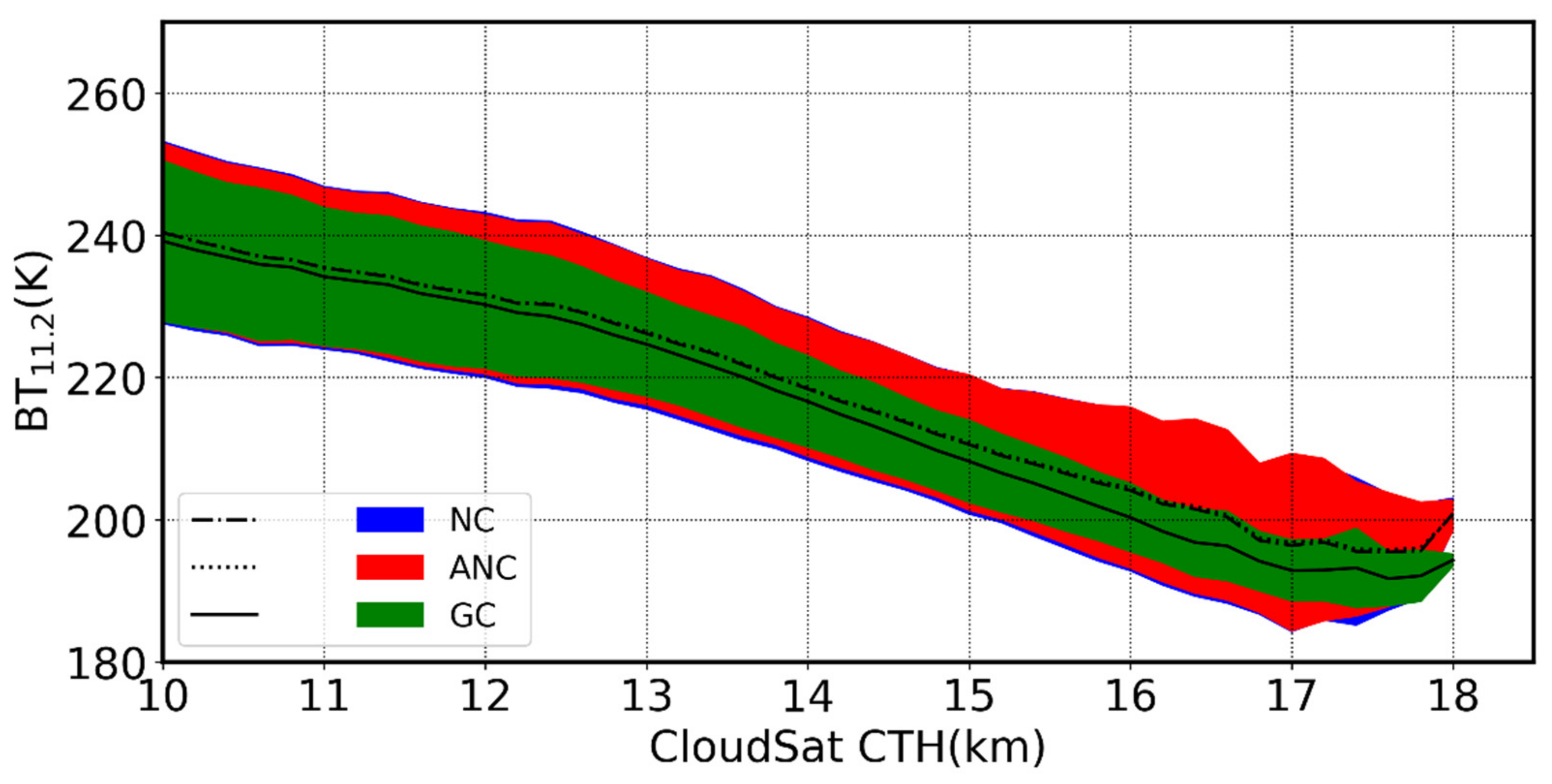
Standard deviation (STD) and the average value of BT 11.2 for every 500 m vertical bin were used for the statistical analyses and a good collocation method should result in a small dispersion of BT 11.2 at each CTH bin for the thick cloud. We excluded multilayer cloud and cirrus to avoid the influence of surface temperature. Figure 3 shows the average BT 11.2 (line) and their STD (shade) of each height bin for deep convection. Both average value and STD of BT 11.2 of ANC (dotted line, read shadow) are almost equal to those of NC (dashed line, blue shadow) at each altitude bin, which means that ANC cannot improve NC remarkably. On the other hand, the GC method reduces the variation of BT 11.2 distinctly for deep convection. The average BT 11.2 from GC (solid line) is also lower than that of NC and ANC as height increases (more than 1 K at 17.5 km). Theoretically, as shown in the functions in Appendix A, the corrected shift of GC is not only related to CTH, but also related to SZA (ranging from 0 to 84°) which indicates the relative distance from the target cloud to the subsatellite point, and SAA which is only related to the transformation from geometric displacement to the geographic coordinate system. The relationship between corrected shift and CTH/SZA is not simply linear but monotonic, and the shift increase with larger CTH/SZA. Only corrected distance of cloud with low CTH and/or small SZA could be neglected. Overall, GC has the advantage over NC and ANC since it considers both the influence of CTH and SZA on the parallax shift of BT 11.2 and the GC-corrected BT 11.2 shows a considerably colder average BT 11.2 as well as smaller STD.
For the GC method, there are still some factors that could introduce errors to collocation, such as spherical earth assumption and cloud overlapping. We tested the impact of earth shape by comparing the difference between corrected displacement by spherical and elliptical earth assumption. The elliptical earth was modeled with the semimajor and semiminor axis defined in the World Geodetic System (WGS84) while the radius of a spherical earth is set to a fixed number (6371 km). For simplicity, we only compared these two earth models for a constant 18 km CTH. Although the difference of corrected shift between the sphere earth model and the elliptical earth becomes larger as SZA increases, it is too small to affect the collocation between HMW8/AHI and CloudSat (Figure S1). As for the overlapping problem, clouds with low CTH and/or large SZA can be overlapped with other clouds on the scan route and it cannot be settled by the GC method. However, error from overlapping could be neglected in this work since we only focus on overshooting clouds with very high CTH (over 14 km at tropics).

4.2. Performance of the RF Model

4.2.1. Feature Selection and Model Tuning

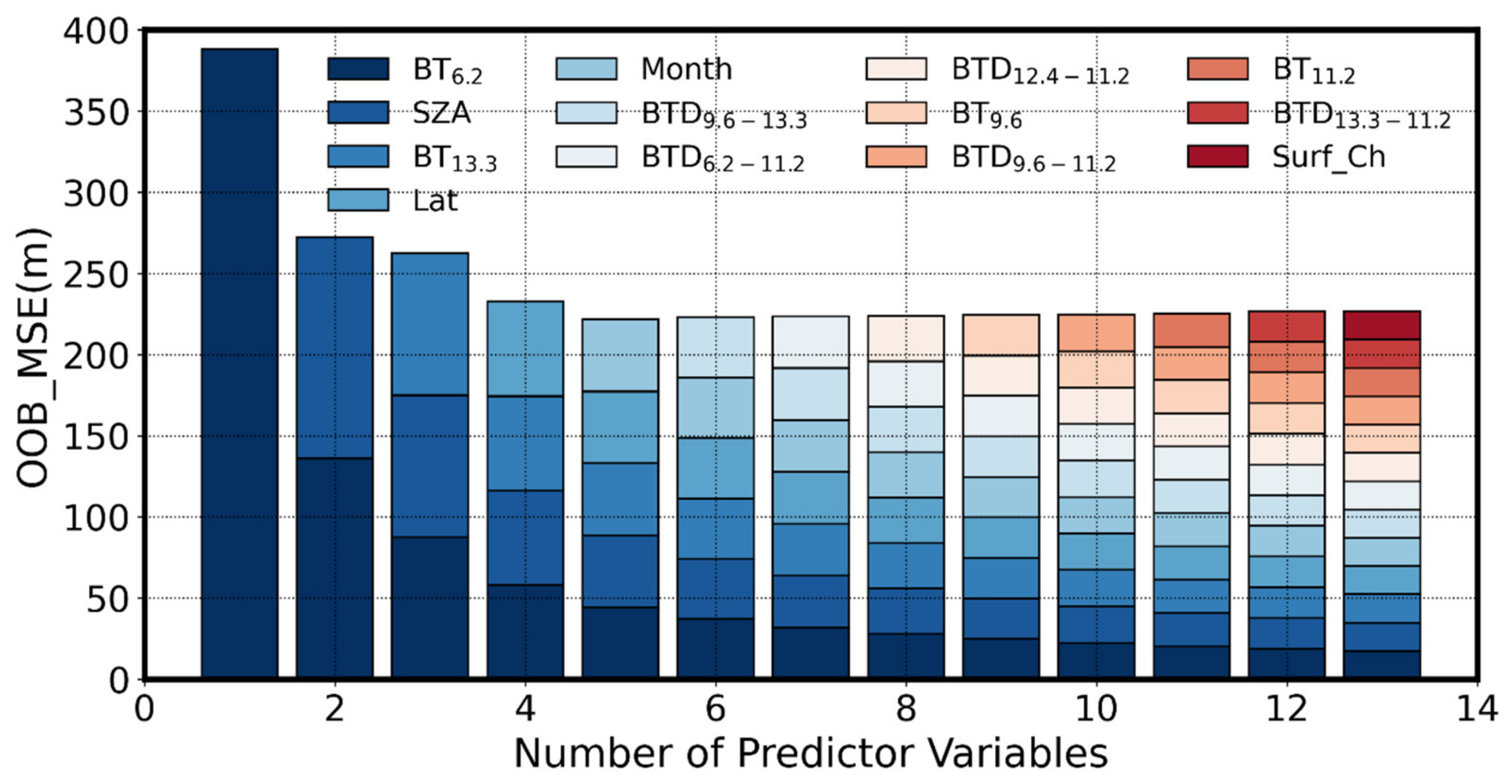
Figure 4 shows the performance of the RF model indicated by OOB_MSE during the SFS procedure and the predictors are sorted in order of descending importance, where colder color indicates greater importance of the variable. A smaller OOB_MSE indicates better accuracy of prediction. The OOB_MSE typically decreases first and then increases slightly again as the subset gets larger. In our case, the feature subset with five predictors has the best performance with the smallest OOB_MSE and this optimal subset of predictors includes BT 6.2 , SZA, BT 13.3 , latitude, and month (descending importance) and is used for subsequent model tuning. The importance of predictors represented by MDA of OOB_MSE are shown in Figure S1 and these five variables have MDA larger than 0.5, which means that the shuffle of any of these five variables could lead to an OOB_MSE increased by as much as 50% from the default model.
Atmospheric window and carbon dioxide absorption channel (11.2 and 13.3 um) have stronger penetration than water vapor absorption channel (6.2 um), and brightness temperature is retrieved from the radiation of different channels from the cloud top, so that BT 6.2 generally indicates brightness temperature of higher altitude, which might be the potential reason for the importance of BT 6.2 . There are three types of penetration convection [6] including ‘cold-high’, ‘cold-low’, and ‘warm-high’ corresponding to the incipient, mature, and dissipating stage of overshooting convection. In this case,   BT 13.3   and BT 11.2 are not the best proxy of cloud-top height especially for ‘warm-high’ types, since they represent the emission that arises from deeper within the cloud as the fall of the convective core, which makes the cloud appear warmer in IR brightness temperature; but the sensitivity to the moisture of 6.2 um channel makes BT 6.2 still represent the height near cloud-top. BT 13.3 is the most commonly used channel to estimate cloud-top height and it just works as a complement of BT 6.2 and could take over BT 6.2 as the dominant predictor if manually excluding BT 6.2 from predictors, but at the price of a little accuracy. Notice that BT 11.2 is less important as shown in Figure S1, its high correlation with BT 13.3 for overshooting clouds (correlation coefficient is 0.98 at 1% significant level) may lead to its importance shared by BT 13.3 . However, BTDs are not important for the estimation of CTH of overshooting clouds in our RF model. Besides, the effect of SZA on the infrared radiance of each pixel causes the impact of SZA on CTH estimation. The spatial and temporal variation of tropopause, latitude, and month are also important for overshooting cloud CTH retrieval.
Parameters including n_tree and max_features can affect the performance of the RF model. To assess the impact of n_tree and max_features on OOB_MSE, a large number of RF models with n_tree ranging from 1 to 1000 using randomly selected subsets (max_features = 1 to 5) were created and Figure 5a provides information about how the model error (OOB_MSE) changes with the n_tree for different max_features. The error of model converges from ≈ 500 trees onwards and a larger number of trees neither increase nor decrease the model accuracy. Considering both accuracy and computation time, n_tree = 500 is large enough and sufficient to produce a stable prediction for this work. Based on the foregoing results about n_tree, OOB_MSE at different max_features of RF models with n_tree = 500 are considered, and the influence of max_features on model error is shown in Figure 5b. When max_features = 3 is selected, OOB_MSE turns to be the smallest value (averaged at 219.25 m), which indicates the highest prediction accuracy.
Since our purpose was testing the feasibility of machine learning in overshooting cloud-top height retrieval, we arranged the feature selection procedure followed by model tuning in this study to save computation expense, and the main parameters were set to default in the feature selection procedure. However, when it comes to operational application, if not caring about the computation cost, we recommend the grid search strategy (or exhaust algorithm), which processes feature section and model tuning simultaneously, to get the optimal subset of predictors and model parameters so to obtain the model with the best accuracy.

4.2.2. Evaluation of the RF Model

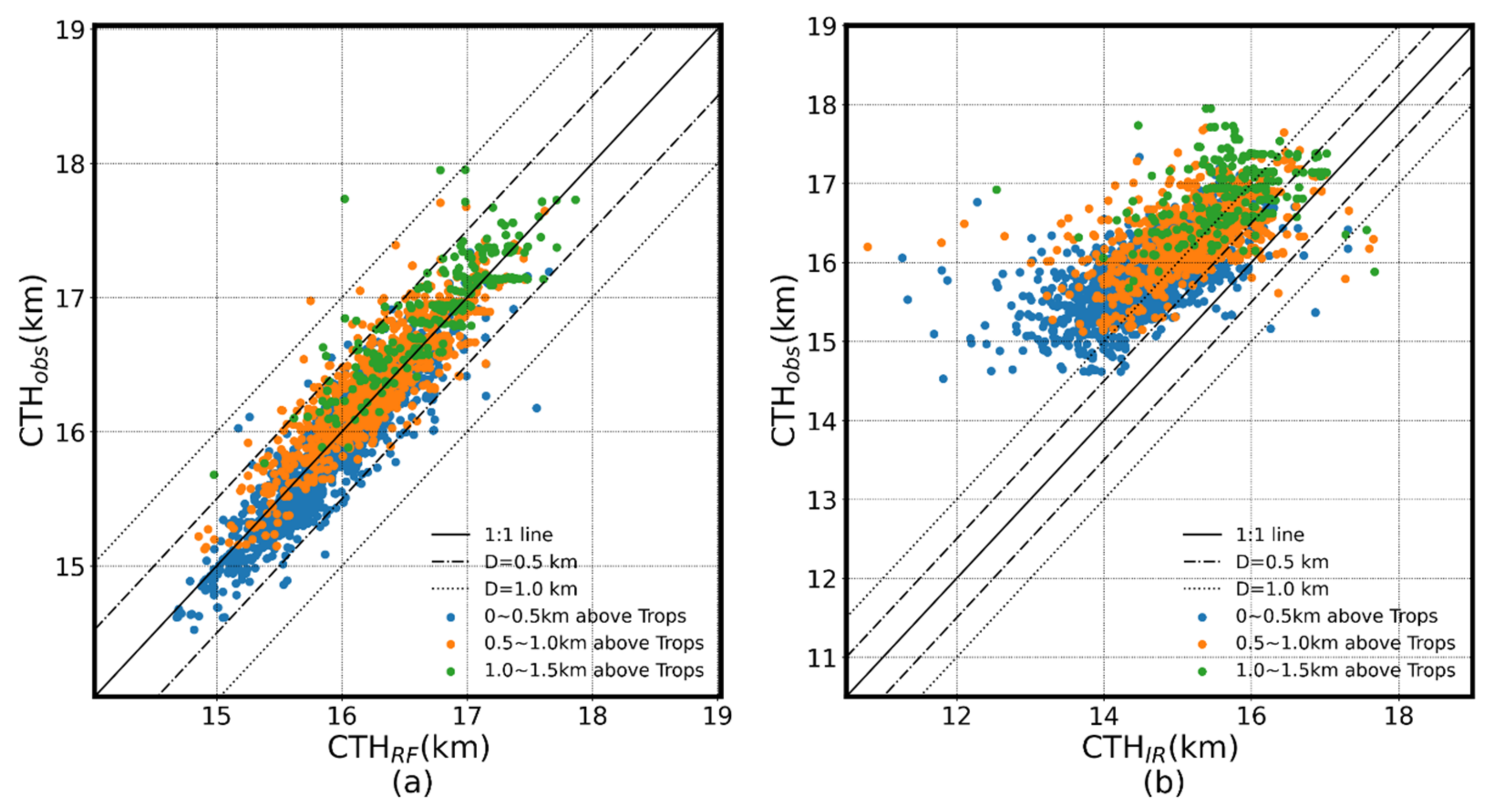
To evaluate the RF model, we compared CTH retrieved from CloudSat ( CTH obs ) and RF model retrieval ( CTH RF ) based on test data and the results are shown in Figure 6a. CTH RF shows good consistency to CTH obs with R = 0.92, RMSE = 222 m, and MAE = 164 m. The frequency distribution of residual between calculated and observed CTH also shows good consistency with 99.3% of the samples having residual smaller than 750 m while 96.9% of total cases have CTH RF within 500 m from CTH obs   (not shown), which is better than previous work [20] that had 65% of geostationary overshooting top heights within ±500 m of the coincident CPR-estimated heights. However, previous work using ML methods in CTH retrieval which treats all kinds of cloud equally in training machine learning method has worse performance with the mean MAE over 1.6 km and most of their error comes from the cloud with CTH > 12 km or CTH < 2 km [19]. Another way to evaluate model performance is based on the overshooting depth represented by the difference between CTH obs and GFS tropopause height. We categorized all cases into three classes based on overshooting depths with bins of 500 m (0–500 m, 500–1 km, above 1 km). The performance of RF model of these three classes was tested, and results show that CTH obs agrees well with CTH RF , with R ranges from 0.85 to 0.91, RMSE ranges from 200 m to 281 m, while MAE ranges from 151 to 281 m from low to high penetration cloud relative to GFS tropopause. When it comes to the performance of the RF model for the extremely high overshooting clouds with cloud-top temperature colder than tropopause temperature which cannot be searched on NWP temperature profile, the result still shows a good agreement with observation (R = 0.86, RMSE = 226 m).

4.2.3. Comparison with Interpolation Method

We applied the most common method for ascertaining CTH from space in real-time by matching the satellite IRBT to the appropriate vertical level within a collocated rawinsonde (temperature profile) from NWP, especially for deep convection which is optically opaque. The infrared window (11.2 μm) brightness temperature taken by the HMW8/AHI was utilized along with the temperature profiles obtained from CloudSat ECMWF-AUX product in this method and the CTH of overshooting clouds from HMW8 pixels were linearly interpolated as the lowest altitude where the temperature profile matched BT 11.2 . For extremely high overshooting clouds (overshooting convective clouds), their cloud-top temperature can be cooler than the environment [20], then their CTHs were calculated by adding the difference between the cloud-top temperature and tropopause temperature divided by the adiabatic lapse rate (9.76 K/km) to the tropopause height, with the assumption that undiluted convective updraft overshoots tropopause and continues to rise adiabatically [6].
We obtained the CTH of test data by the interpolation method described above as shown in Figure 6b, and the CTH retrieved from the single-channel interpolation method ( CTH IR ) has larger discrepancies than CTH RF , with R of 0.70. CTH IR   shows significant underestimates for most samples, with RMSE and MAE more than 1 km (1305 and 1179 m); The result is similar to the work of Min et al. [19] which showed that CTHs products of HMW8 proposed by the Japan Meteorological Agency (JMA, Tokyo, Japan) [18,59], which uses the combination of the interpolation method, radiance ratioing method, and intercept method, have significant underestimates with almost ≈5 km lower than that observed from Cloud Physics Lidar (CPL) [19]. Even though they contribute the underestimation to the undetectably thin and high cloud layers, it has already shown pronounced underestimation when CTH > 12 km. For the peer comparison, we calculated R, RMSE, and MAE of three classes based on overshooting depths. CTHs estimates at each 500 m bins above GFS tropopause show less accuracy with R ranging from 0.35 to 0.63, RMSE from 1274 to 1324 m, and MAE from 1126 to 1208 m in comparison with that of RF model with R ranges from 0.85 to 0.91, RMSE ranges from 200 to 281 m, while MAE ranges from 151 to 281 m.
The traditional method holds an assumption that the cloud temperature is the same as that of the environment at the same altitude. Even though the temperature contrast between cloud-top and environment generally becomes smaller towards higher altitude due to adiabatic cooling and mixing. However, when it comes to specific events, it varies based on different conditions, and, for most cases, the convective thermals still tend to be warmer than the environment, which might be the reason for its underestimate. However, as for the RF model, we took all variables related to overshooting events into consideration, including variables about tropopause such as latitude and month, variables related to cloud-top properties such as cloud-top brightness temperature, as well as, even though excluded in the final model, variables related to the strength of convection such as BTDs, etc., and the RF model learns the relationship between CTH and all predictors, which indicates that the predictability of the RF model comes from the combination of all these relationships without any pre-existing assumption. However, there is an inherent shortcoming of the data-driven ML method that it can only learn rules from data on hand, and the accuracy of the model is somehow affected by the sample size, therefore, it is very important for data collection in our future work.

5. Conclusions

Errors in the nearest matching method (NC) for the collocation between HMW8/AHI and CloudSat data produce anomalously high/low values of B T 11.2 and significant mismatch especially for tall cloud. The 3 × 3-pixel-average method (ANC) cannot decrease this error. A simplified collocation method, which considers geometric displacement and utilizes spherical earth assumption, was used in the data collocation. As shown in the theoretical analysis (functions in Appendix A), parallax displacement is related to both CTH and SZA, and their relationship is monotonic. Only for the cloud with small CTH and SZA, the geometric shift could be neglected. Results show that the HMW8/AHI cloud-top B T 11.2 agrees better with the structure of CloudSat reflectivity after geometric collocation in both case study and statistical analysis.
After collocation, we used the RF model based on IR indicators from the HMW8/AHI satellite along with some temporal and geographic factors as predictors to test the applicability of the machine learning model in overshooting cloud-top height retrieval. After the SFS procedure and model tuning, the RF model was finally constructed with n_tree = 500 and max_feature = 3 from five predictors ( B T 6.2 , SZA, B T 13.3 , latitude, and month). Basically, the prediction provided by the RF model was calculated by combining relationships between overshooting CTH and all predictors. Results show that the RF model is an effective and valid method in calculating CTH of overshooting clouds with low error (small RMSE and MAE around 200 m) and higher correlation (R = 0.92), even as for cases over 1 km above the tropopause, their CTH retrieved from the RF model still highly correlated to observations with R = 0.85. However, the traditional single-channel interpolation method has a much lower correlation of 0.7 and larger RMSE and MAE over 1 km. Results verify the applicability of machine learning for CTH retrieval of overshooting clouds.
Overall, this work provides a preliminary application of CTH estimation with the machine learning method and obtains good accuracy. However, some shortcomings remain unsettled, for example, model error increases as increasing CTH, which is the result of decreasing sample size of overshooting clouds. What we used for the RF model was overshooting cases so that the bias from decreasing sample size is still acceptable, but it is noteworthy to mention that larger sample size is necessary to improve the accuracy. Considering the larger spatial coverage of more advanced radars onboard TRMM/GPM satellite [60] which could provide a near-global view of 3D cloud structure in 2–3 h, as well as other active sensors such as CALIPSO, one of our main ongoing efforts is collecting more samples by combining these advanced radars with HMW8 to improve the accuracy of the model. More algorithms other than RF, such as neural networks, will be implemented and assessed with data from different geostationary satellites and their application to CTH retrieval based on cloud types to produce a global product of CTH retrieval in our future works. Additionally, it is also of good possibility for machine learning methods, along with the overshooting detection method for geo-satellites, to be promoted to geo-satellites other than HMW8, such as GOES-R, for the real-time and global analyses of penetration cloud height for a variety of weather and climate applications in the future work.

Supplementary Materials

The following are available online at https://www.mdpi.com/2073-4433/12/2/173/s1. Figure S1: The importance of candidate predictors ordered by MDA of MSE.

Author Contributions

Conceptualization, G.W. and H.W.; methodology, G.W. and Y.Z.; software, G.W. and H.K.; validation, S.C.; formal analysis, G.W., H.W., and Y.Z.; investigation, G.W.; resources, G.W. and Y.Z.; data curation, G.W. and S.C.; writing—original draft preparation, G.W.; writing—review and editing, G.W., H.W., and Y.Z.; visualization, G.W.; supervision, H.W., Y.Z., and Q.W.; project administration, H.W.; funding acquisition, H.W. and Q.W. All authors have read and agreed to the published version of the manuscript.

Funding

This research was funded by the China Special Fund for Meteorological Research in the Public Interest (Grant No: GYHY201306047) and Youth Program of National Natural Science Foundation of China (Grant No:42005111), and the author G.W. was additionally funded by the China Scholarship Council (CSC; 201806010052).

Institutional Review Board Statement

Not applicable.

Informed Consent Statement

Not applicable.

Data Availability Statement

Data is contained within the article or supplementary material.

Acknowledgments

The authors are grateful to the Japan Aerospace Exploration Agency (JAXA) Himawari Monitor (p-tree system) for providing the Himawari-8/AHI L1 Gridded data, the CloudSat Data Processing Center for providing the CloudSat data, and the NCEP for providing GFS data. Additionally, we also thank the anonymous reviewers for their suggestions for improving the manuscript.

Conflicts of Interest

The authors declare no conflict of interest.

Appendix A

As shown in Figure A1, referring to the parallax correction method given by [42], assuming S CPR as CloudSat CPR and S AHI as Geo-satellite Himawari-8/AHI, A observes cloud-top at point F with a ground footprint of CloudSat at point D, and B observes the same cloud-top with ground footprint E. To make sure that the information from the geo-satellite sensor correctly matches that of CloudSat, a shift in the ground footprint of B is required and the correct shift is related to some factors including satellite zenith angle, the altitude of instrument A, cloud-top height, etc. Besides, we denote satellite zenith angle (SZA, ∠AD S AHI ) as   α , satellite viewing angle (SVA, ∠O S AHI D) as β . Assuming that earth is a sphere with constant averaging real earth radius ( L OD =   =   Re , ~6371 km), distance from earth’s center to the satellite (DES) is constant ( L OB , ~ km) as well.
Using sine law in ΔDO S AHI , ΔFD S AHI , and ΔEO S AHI , then we get
β = sin 1 ( L OD sin α L OS AHI )
OFS AHI = sin 1 L OB sin α     β L FS AHI
OES AHI = sin 1 L OB L OF sin α     β L FS AHI L OE
Using cosine law in ΔFD S AHI , we could easily get
L FS AHI = L DF 2 + L DS AHI 2     2 * L DF * L DS AHI * cos α
L ED ^ = Re * DOE = Re * ( sin 1 L OB sin α     β L FS AHI     sin 1 L OS AHI L OF sin α     β L FS AHI L OE )
L OF is the distance from the cloud-top to the earth’s center, which is the sum of earth radius and cloud-top height. The direction of L ED ^ is given by the satellite azimuth angle   SAA , φ , the angle between a vector L ED ^ and local geodetic north. Denote the latitude and longitude of point D as LAT D and LON D in radians, then the latitude and longitude of E could be written as
LAT E   = LAT D   + L ED * cos φ / Re
LON E = LON D + L ED * sin φ / ( Re * cos LAT D )
Figure A1. Schematic representation of viewing geometries from space-to-earth view for two satellites of HMW8/AHI (satellite S AHI ) and CloudSat (satellite S CPR ) for the deep convective cloud. C is the subsatellite point of HMW8/AHI on the equator and D, the footprint of deep convective cloud, could be at any location.
Atmosphere 12 00173 g0a1

References

  1. Wang, P.K. Moisture plumes above thunderstorm anvils and their contributions to cross-tropopause transport of water vapor in midlatitudes. J. Geophys. Res. Atmos. 2003. [Google Scholar] [CrossRef] [Green Version]
  2. Rosenlof, K.H. How Water Enters the Stratosphere. Science 2003, 302, 1691–1692. [Google Scholar] [CrossRef] [PubMed]
  3. Devasthale, A.; Fueglistaler, S. A climatological perspective of deep convection penetrating the TTL during the Indian summer monsoon from the AVHRR and MODIS instruments. Atmos. Chem. Phys. 2010. [Google Scholar] [CrossRef] [Green Version]
  4. James, R.; Bonazzola, M.; Legras, B.; Surbled, K.; Fueglistaler, S. Water vapor transport and dehydration above convective outflow during Asian monsoon. Geophys. Res. Lett. 2008. [Google Scholar] [CrossRef] [Green Version]
  5. Pan, L.L.; Homeyer, C.R.; Honomichl, S.; Ridley, B.A.; Weisman, M.; Barth, M.C.; Hair, J.W.; Fenn, M.A.; Butler, C.; Diskin, G.S.; et al. Thunderstorms enhance tropospheric ozone by wrapping and shedding stratospheric air. Geophys. Res. Lett. 2014. [Google Scholar] [CrossRef]
  6. Luo, Z.; Liu, G.Y.; Stephens, G.L. CloudSat adding new insight into tropical penetrating convection. Geophys. Res. Lett. 2008. [Google Scholar] [CrossRef] [Green Version]
  7. Bedka, K.; Brunner, J.; Dworak, R.; Feltz, W.; Otkin, J.; Greenwald, T. Objective satellite-based detection of overshooting tops using infrared window channel brightness temperature gradients. J. Appl. Meteorol. Climatol. 2010. [Google Scholar] [CrossRef]
  8. Lane, T.P.; Sharman, R.D.; Clark, T.L.; Hsu, H.M. An investigation of turbulence generation mechanisms above deep convection. J. Atmos. Sci. 2003. [Google Scholar] [CrossRef]
  9. Smith, W.L.; Minnis, P.; Finney, H.; Palikonda, R.; Khaiyer, M.M. An evaluation of operational GOES-derived single-layer cloud top heights with ARSCL data over the ARM Southern Great Plains Site. Geophys. Res. Lett. 2008. [Google Scholar] [CrossRef] [Green Version]
  10. Wang, Z.; Wang, Z.; Cao, X.; Tao, F. Comparison of cloud top heights derived from FY-2 meteorological satellites with heights derived from ground-based millimeter wavelength cloud radar. Atmos. Res. 2018. [Google Scholar] [CrossRef]
  11. Dworak, R.; Bedka, K.; Brunner, J.; Feltz, W. Comparison between GOES-12 overshooting-top detections, WSR-88D radar reflectivity, and severe storm reports. Weather Forecast. 2012. [Google Scholar] [CrossRef] [Green Version]
  12. Liu, C.; Zipser, E.J. Global distribution of convection penetrating the tropical tropopause. J. Geophys. Res. Atmos. 2005. [Google Scholar] [CrossRef] [Green Version]
  13. Zipser, E.J.; Cecil, D.J.; Liu, C.; Nesbitt, S.W.; Yorty, D.P. Where are the most: Intense thunderstorms on Earth? Bull. Am. Meteorol. Soc. 2006. [Google Scholar] [CrossRef] [Green Version]
  14. Wang, J.; Houze, R.A.; Fan, J.; Brodzik, S.R.; Feng, Z.; Hardin, J.C. Under a Creative Commons Attribution 4.0 InternationThe Detection of Mesoscale Convective Systems by the GPM Ku-Band Spaceborne Radar. J. Meteorol. Soc. Jpn. 2019, 97, 1059–1073. [Google Scholar] [CrossRef] [Green Version]
  15. Young, A.H.; Bates, J.J.; Curry, J.A. Complementary use of passive and active remote sensing for detection of penetrating convection from CloudSat, CALIPSO, and Aqua MODIS. J. Geophys. Res. Atmos. 2012. [Google Scholar] [CrossRef]
  16. Weisz, E.; Li, J.; Menzel, W.P.; Heidinger, A.K.; Kahn, B.H.; Liu, C.Y. Comparison of AIRS, MODIS, CloudSat and CALIPSO cloud top height retrievals. Geophys. Res. Lett. 2007. [Google Scholar] [CrossRef]
  17. Chae, J.H.; Sherwood, S.C. Insights into Cloud-top height and Dynamics from the Seasonal cycle of cloud-top heights observed by MISR in the west Pacific region. J. Atmos. Sci. 2010. [Google Scholar] [CrossRef] [Green Version]
  18. Kouki, M.; Hiroshi, S.; Ryo, Y.; Toshiharu, I. Algorithm Theoretical Basis Document for Cloud Top Height Product; Technical Note, No.61; Meteorological Satellite Center: Tokyo, Japan, 2016. [Google Scholar]
  19. Min, M.; Li, J.; Wang, F.; Liu, Z.; Menzel, W.P. Retrieval of cloud top properties from advanced geostationary satellite imager measurements based on machine learning algorithms. Remote Sens. Environ. 2020, 239. [Google Scholar] [CrossRef]
  20. Griffin, S.M.; Bedka, K.M.; Velden, C.S. A method for calculating the height of overshooting convective cloud tops using satellite-based IR imager and CloudSat cloud profiling radar observations. J. Appl. Meteorol. Climatol. 2016. [Google Scholar] [CrossRef]
  21. Wylie, D.P.; Santek, D.; Starr, D.O.C. Cloud-top heights from GOES-8 and GOES-9 stereoscopic imagery. J. Appl. Meteorol. 1998. [Google Scholar] [CrossRef]
  22. Lee, J.; Shin, D.-B.; Chung, C.-Y.; Kim, J. A Cloud Top-Height Retrieval Algorithm Using Simultaneous Observations from the Himawari-8 and FY-2E Satellites. Remote Sens. 2020. [Google Scholar] [CrossRef]
  23. Kaňák, J.; Bedka, K.M.; Sokol, A. (PDF) Mature Convective Storms and Their Overshooting Tops over Central Europe—Overshooting Top Height Analysis for Summers 2009–2011. Available online: https://www.researchgate.net/publication/269100731_MATURE_CONVECTIVE_STORMS_AND_THEIR_OVERSHOOTING_TOPS_OVER_CENTRAL_EUROPE_-_OVERSHOOTING_TOP_HEIGHT_ANALYSIS_FOR_SUMMERS_2009-2011 (accessed on 28 November 2020).
  24. Xiang, B.; Zeng, C.; Dong, X.; Wang, J. The application of a decision tree and stochastic forest model in summer precipitation prediction in Chongqing. Atmosphere 2020. [Google Scholar] [CrossRef]
  25. Feng, C.; Zhang, X.; Wei, Y.; Zhang, W.; Hou, N.; Xu, J.; Jia, K.; Yao, Y.; Xie, X.; Jiang, B.; et al. Estimating Surface Downward Longwave Radiation Using Machine Learning Methods. Atmosphere 2020, 11, 1147. [Google Scholar] [CrossRef]
  26. Taheri Shahraiyni, H.; Sodoudi, S. Statistical Modeling Approaches for PM10 Prediction in Urban Areas; A Review of 21st-Century Studies. Atmosphere 2016, 7, 15. [Google Scholar] [CrossRef] [Green Version]
  27. Xu, W.; Ning, L.; Luo, Y. Wind speed forecast based on post-processing of numerical weather predictions using a gradient boosting decision tree algorithm. Atmosphere 2020. [Google Scholar] [CrossRef]
  28. Pawlak, I.; Jarosławski, J. Forecasting of Surface Ozone Concentration by Using Artificial Neural Networks in Rural and Urban Areas in Central Poland. Atmosphere 2019, 10, 52. [Google Scholar] [CrossRef] [Green Version]
  29. Zhou, K.; Zheng, Y.; Li, B.; Dong, W.; Zhang, X. Forecasting Different Types of Convective Weather: A Deep Learning Approach. J. Meteorol. Res. 2019, 33, 797–809. [Google Scholar] [CrossRef]
  30. Häkansson, N.; Adok, C.; Thoss, A.; Scheirer, R.; Hörnquist, S. Neural network cloud top pressure and height for MODIS. Atmos. Meas. Tech. 2018. [Google Scholar] [CrossRef] [Green Version]
  31. Okuyama, A.; Andou, A.; Date, K.; Hoasaka, K.; Mori, N.; Murata, H.; Tabata, T.; Takahashi, M.; Yoshino, R.; Bessho, K. Preliminary validation of Himawari-8/AHI navigation and calibration. In Proceedings of the Earth Observing Systems XX; Butler, J.J., Xiong, X., Gu, X., Eds.; SPIE: Bellingham, WA, USA, 2015; Volume 9607, p. 96072E. [Google Scholar]
  32. Bessho, K.; Date, K.; Hayashi, M.; Ikeda, A.; Imai, T.; Inoue, H.; Kumagai, Y.; Miyakawa, T.; Murata, H.; Ohno, T.; et al. An introduction to Himawari-8/9—Japan’s new-generation geostationary meteorological satellites. J. Meteorol. Soc. Jpn. 2016, 94, 151–183. [Google Scholar] [CrossRef] [Green Version]
  33. Shang, H.; Chen, L.; Letu, H.; Zhao, M.; Li, S.; Bao, S. Development of a daytime cloud and haze detection algorithm for Himawari-8 satellite measurements over central and eastern China. J. Geophys. Res. 2017. [Google Scholar] [CrossRef]
  34. Kurihara, Y.; Murakami, H.; Kachi, M. Sea surface temperature from the new Japanese geostationary meteorological Himawari-8 satellite. Geophys. Res. Lett. 2016. [Google Scholar] [CrossRef] [Green Version]
  35. Mace, G. Level 2 GEOPROF Product Process Description and Interface Control Document; Cooperative Institute for Research in the Atmosphere; Colorado State University: Fort Collins, CO, USA, 2004; pp. 1–20. [Google Scholar]
  36. Hoinka, K.P. The tropopause: Discovery, definition and demarcation. Meteorol. Zeitschrift 1997. [Google Scholar] [CrossRef]
  37. Pan, L.L.; Hintsa, E.J.; Stone, E.M.; Weinstock, E.M.; Randel, W.J. The seasonal cycle of water vapor and saturation vapor mixing ratio in the extratropical lowermost stratosphere. J. Geophys. Res. Atmos. 2000. [Google Scholar] [CrossRef] [Green Version]
  38. Homeyer, C.R.; Bowman, K.P.; Pan, L.L. Extratropical tropopause transition layer characteristics from high-resolution sounding data. J. Geophys. Res. Atmos. 2010. [Google Scholar] [CrossRef] [Green Version]
  39. Pan, L.L.; Munchak, L.A. Relationship of cloud top to the tropopause and jet structure from CALIPSO data. J. Geophys. Res. Atmos. 2011. [Google Scholar] [CrossRef]
  40. Sherwood, S.C.; Chae, J.H.; Minnis, P.; McGill, M. Underestimation of deep convective cloud tops by thermal imagery. Geophys. Res. Lett. 2004. [Google Scholar] [CrossRef] [Green Version]
  41. Chung, E.S.; Sohn, B.J.; Schmetz, J. CloudSat shedding new light on high-reaching tropical deep convection observed with Meteosat. Geophys. Res. Lett. 2008. [Google Scholar] [CrossRef]
  42. Wang, C.; Luo, Z.J.; Huang, X. Parallax correction in collocating CloudSat and Moderate Resolution Imaging Spectroradiometer (MODIS) observations: Method and application to convection study. J. Geophys. Res. 2011, 116, D17201. [Google Scholar] [CrossRef] [Green Version]
  43. Kühnlein, M.; Appelhans, T.; Thies, B.; Nauss, T. Improving the accuracy of rainfall rates from optical satellite sensors with machine learning—A random forests-based approach applied to MSG SEVIRI. Remote Sens. Environ. 2014. [Google Scholar] [CrossRef] [Green Version]
  44. Hamidi, O.; Tapak, L.; Abbasi, H.; Maryanaji, Z. Application of random forest time series, support vector regression and multivariate adaptive regression splines models in prediction of snowfall (a case study of Alvand in the middle Zagros, Iran). Theor. Appl. Climatol. 2018. [Google Scholar] [CrossRef]
  45. Yao, J.; Raffuse, S.M.; Brauer, M.; Williamson, G.J.; Bowman, D.M.J.S.; Johnston, F.H.; Henderson, S.B. Predicting the minimum height of forest fire smoke within the atmosphere using machine learning and data from the CALIPSO satellite. Remote Sens. Environ. 2018. [Google Scholar] [CrossRef]
  46. Liaw, A.; Wiener, M. Classification and Regression by randomForest. R News 2002, 2, 18–22. [Google Scholar]
  47. Cutler, A.; Cutler, D.R.; Stevens, J.R. Random forests. In Ensemble Machine Learning: Methods and Applications; Springer: Boston, MA, USA, 2012; ISBN 9781441993267. [Google Scholar]
  48. Boulesteix, A.L.; Janitza, S.; Kruppa, J.; König, I.R. Overview of random forest methodology and practical guidance with emphasis on computational biology and bioinformatics. Wiley Interdiscip. Rev. Data Min. Knowl. Discov. 2012. [Google Scholar] [CrossRef] [Green Version]
  49. Breiman, L. Bagging predictors. Mach. Learn. 1996. [Google Scholar] [CrossRef] [Green Version]
  50. Kwon, E.H.; Sohn, B.J.; Schmetz, J.; Watts, P. Intercomparison of height assignment methods for opaque clouds over the tropics. Asia-Pac. J. Atmos. Sci. 2010, 46, 11–19. [Google Scholar] [CrossRef]
  51. Olander, T.L.; Velden, C.S. Tropical cyclone convection and intensity analysis using differenced infrared and water vapor imagery. Weather Forecast. 2009. [Google Scholar] [CrossRef] [Green Version]
  52. Schmetz, J.; Tjemkes, S.A.; Gube, M.; Van De Berg, L. Monitoring deep convection and convective overshooting with METEOSAT. Adv. Space Res. 1997. [Google Scholar] [CrossRef]
  53. Kwon, E.H.; Sohn, B.J.; Schmetz, J.; Watts, P. Use of ozone channel measurements for deep convective cloud height retrievals over the tropics. In Proceedings of the 16th Conference on Satellite Meteorology and Oceanography, Phoenix, AZ, USA, 11–15 January 2009. [Google Scholar]
  54. Hamada, A.; Nishi, N. Observation-based estimation of cloud-top height by geostationary satellite split-window measurements trained with CloudSat data. In Remote Sensing and Modeling of the Atmosphere, Oceans, and Interactions III; SPIE: Bellingham, WA, USA, 2010. [Google Scholar]
  55. Iguyon, I.; Elisseeff, A. An introduction to variable and feature selection. J. Mach. Learn. Res. 2003, 3, 1157–1182. [Google Scholar]
  56. Rodriguez-Galiano, V.F.; Luque-Espinar, J.A.; Chica-Olmo, M.; Mendes, M.P. Feature selection approaches for predictive modelling of groundwater nitrate pollution: An evaluation of filters, embedded and wrapper methods. Sci. Total Environ. 2018. [Google Scholar] [CrossRef]
  57. Breiman, L. Random forests. Mach. Learn. 2001. [Google Scholar] [CrossRef] [Green Version]
  58. Adler, R.F.; Markus, M.J.; Fenn, D.D.; Szejwach, G.; Shenk, W.E. Thunderstorm top structure observed by aircraft overflights with an infrared radiometer. J. Clim. Appl. Meteorol. 1983. [Google Scholar] [CrossRef] [Green Version]
  59. Kouki, M. Improvement of the Cloud Top Height Algorithm for the Fundamental Cloud Product and Related Evaluation. Available online: https://www.data.jma.go.jp/mscweb/technotes/msctechrep64-3.pdf (accessed on 27 January 2021).
  60. Houze, R.A.; Rasmussen, K.L.; Zuluaga, M.D.; Brodzik, S.R. The variable nature of convection in the tropics and subtropics: A legacy of 16 years of the Tropical Rainfall Measuring Mission satellite. Rev. Geophys. 2015, 53, 994–1021. [Google Scholar] [CrossRef] [PubMed]
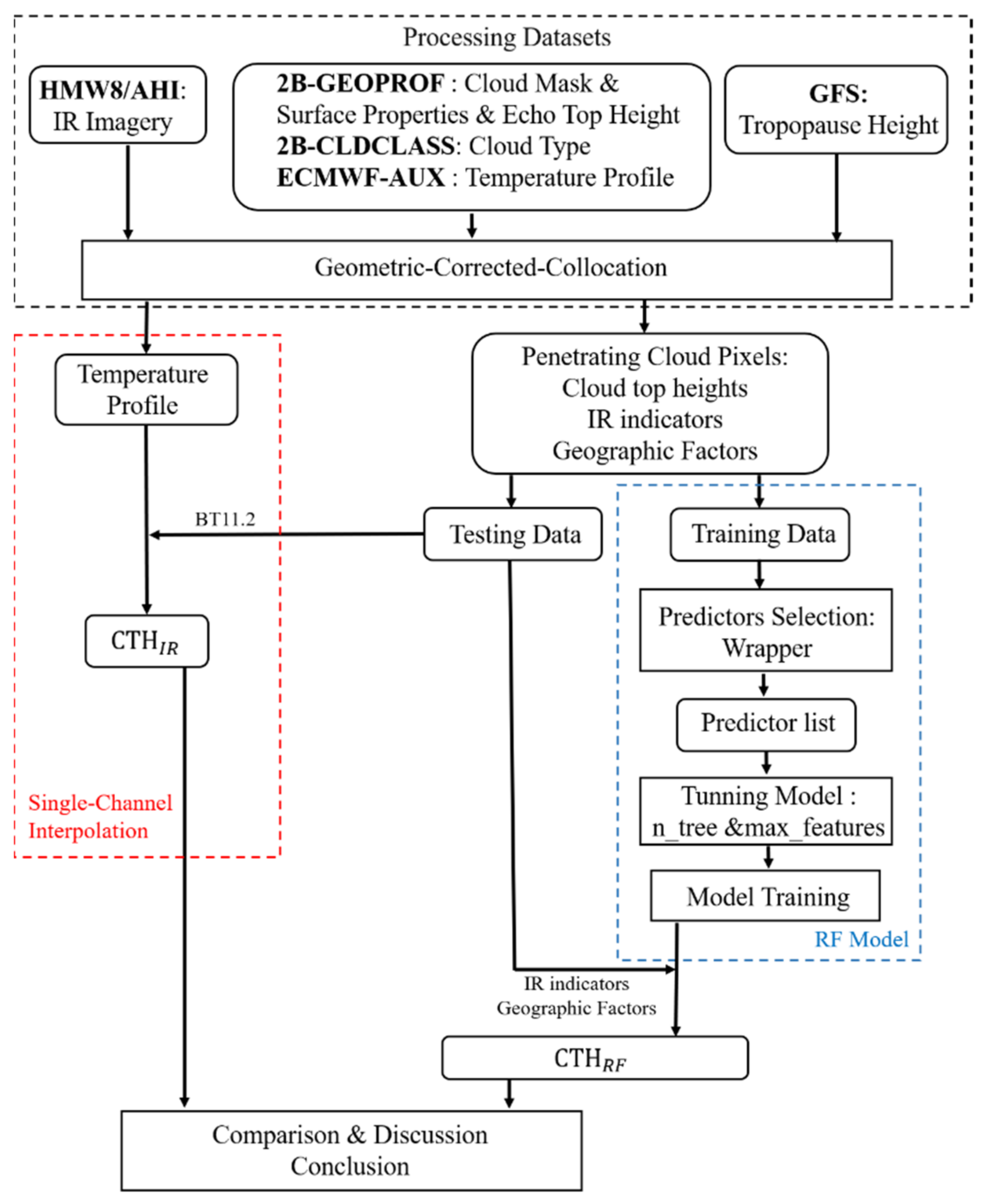
Figure 1. The workflow of this study.
Atmosphere 12 00173 g001
Figure 2. (a) HMW8/AHI 11.2 um brightness temperature ( BT 11.2 ) observed at 7:40 UTC on 28 February 2017 centering at 91° E, 8° N. The blue line is the CloudSat ground track and the red dotted line is the location after geometrical correction. (b) The corresponding CloudSat CPR reflectivity with cloud mask value > 30. (c) HMW8/AHI BT 11.2 along nearest pixels of CloudSat footprint (blue line, NC), 3 × 3 pixels averaging centered at the nearest pixel of CloudSat footprint (blue dotted line, ANC), and footprint after geometrical correction (red line, GC), CTHs based on the traditional method from BT 11.2 of three methods are shown in panel (b). The region between the two vertical bold dotted lines indicates cloud penetrating tropopause.
Atmosphere 12 00173 g002
Figure 3. Standard deviation and the average value of BT 11.2 as the function of CloudSat CTH. Three kinds of lines indicate the average value while shadows of different colors (blue, red, and green) show the STD of BT 11.2 from NC, ANC, and GC methods.
Atmosphere 12 00173 g003
Figure 4. OOB_MSE as a function of the number of variables in subsets which are represented in each column; all variables are ranked with regards to their importance in descending order, and variables with less importance are along with warmer color.
Atmosphere 12 00173 g004
Figure 5. (a) OOB_MSE as a function of the number of trees, colors indicate the different value of max_features, and the red line shows where n_tree = 500; (b) statistical characteristics of OOB_MSE as a function of max_features when n_tree = 500. The box extends from the lower to upper quartile values of the data with a line at the median, and the whiskers extend from the box to show the range of the data while outliers are shown as flier points.
Atmosphere 12 00173 g005
Figure 6. (a) Comparison of CTH from RF model and CloudSat; (b) comparison of CTH from the traditional single-channel interpolation method and CloudSat. Green, orange, and blue dots represent overshooting cloud-top height with overshooting depths of 0–500 m, 500–1 km, and above 1 km separately. The black dashed line represents the 1:1 line while the dash and the dotted line represent the residual between calculated and observed CTH of 500 m and 1 km, respectively.
Atmosphere 12 00173 g006
Table 1. List of candidate predictors.
Variable TypeCandidate PredictorsAbbreviation
Infrared brightness TemperatureIRBT of O3, IRW, CO2, absorption channelsBT9.6, BT11.2, BT13.3
IRBT of water vapor absorption channelBT6.2
Brightness temperature differencesBTD between WV and IRWBTD6.2–11.2
BTD between two IRWsBTD13.3–11.2
BTD between O3 and IRWBTD9.6–11.2
Geographic factorsSeasonal (Month), latitude, SZA,
surface character
Month, Lat, SZA,
Surf Ch,
Publisher’s Note: MDPI stays neutral with regard to jurisdictional claims in published maps and institutional affiliations.