Abstract
A method to detect the atmospheric turbulent layers using a single Shack–Hartmann wavefront sensor is discussed. In order to determine the height distribution of the atmospheric turbulence above a telescope, we register the wavefront distortions at different regions of the aperture from a single light solar object moving in time. Changes of the spatial position of the solar object on the sky give us the possibility to estimate the angular shift of an object. Cross-correlation analysis of the low-frequency component of wavefront slopes spaced on the telescope aperture at different times allows us to estimate characteristics for different atmospheric layers. Knowledge of the height profiles of atmospheric turbulence as well as the Fried parameter is critical for wide-field adaptive optics (AO).
1. Introduction
Turbulent fluctuations of both air temperature and wind speed induce variations in the air refractive index. The study of the atmospheric turbulence and its optical properties is important for astroclimatic research, planning time of astronomical observations as well as searching for the physical mechanisms of optical turbulence evolution. Especially, the study of the bottom part of the atmospheric boundary layer over rough terrain is relevant.
In rough terrain, the structure of the turbulence is broken. Arising wave and vortex disturbances and mesoscale airflows may induce the intense turbulence and variations in the exchange of heat, momentum, and mass. The paper is aimed at the development of the method to detect the turbulence layers. This is important for the study of the structure of optical turbulence at the sites of the Large Solar Vacuum Telescope of the Baikal Astrophysical Observatory as well as Sayan Solar Observatory [1,2].
Atmospheric turbulence can be generated in the atmospheric layers located at different distances from the telescope aperture [3,4,5,6]. Detailed knowledge of the profiles of the atmospheric turbulence is critical for both single-conjugate systems and wide-field solar adaptive optics [7,8,9]. The performance of the AO system depends on the atmospheric turbulence parameters. The integral of height profile of the structure constant of air refractive index determines the key well-known characteristics relevant for AO: Fried parameter, isoplanatic angle and coherent time. Furthermore, it is shown that optical turbulence generated in the vicinity of low-level jet stream (in ∼100–500 m layer) at the Large Solar Vacuum Telescope site induces decrease of the Fried parameter by 1.5 cm, on average [10]. Wide-field AO systems are technologies that correct the wavefront distortions over an extended field of view, for example, by means of deformable mirrors conjugated with various altitudes in the atmosphere and applying atmospheric tomography methods. It is likely that knowledge of even the height profiles of the mean characteristics of turbulence may help in the refinement of tomographic matrices in the reconstruction of 3D wavefront distortions.
There are several techniques for the measurements of the profiles of atmospheric turbulence [11,12,13,14,15,16,17]. The most widely used are Multi-Aperture Scintillation Systems (Mass) [11], Scintillation Detection and Ranging (Scidar) [12,13] and Solar Differential Image Motion Monitors (S-Dimm+) [14]. Furthermore, in order to recover the profiles, the atmospheric turbulence Slope Detection and Ranging (Slodar) technique is used [15,16]. Examples of Slodar turbulence profiles for astronomical observatories are shown in [18,19]. It should be noted that the profiles of the turbulence may be recovered using the Slodar technique with a very high space resolution (10 m or less) only in the surface layer of the atmosphere (up to ∼50 m) [19]. Vertical resolution in the upper atmospheric layers is significantly reduced.
Slodar and Scidar are triangulation techniques in which the profiles of the atmospheric turbulent parameters are recovered from either cross-correlation analysis of the small-scale wavefront slopes or cross-correlation of scintillation intensity patterns, respectively. Nevertheless, there are differences in the estimates of the parameters of atmospheric turbulence (including the structure constant of air refractive index , Fried parameter , outer scale of turbulence ) at different altitudes in Slodar and G-Scidar techniques. A comparison between the Scidar and Slodar techniques is performed in [20].
2. Slodar Technique
Data of measurements [21] show that spatial distribution of characteristics at the telescope aperture is not random. Distribution of wavefront local slopes on the telescope aperture is determined by the character of height profiles of the atmospheric optical and dynamic turbulence. Cross-correlation analysis of local wavefront slopes on the aperture is the basis of atmospheric turbulence profiling by Slodar-based techniques [15]. In order to understand the features of distribution of small-scale wavefront distortions at the aperture we consider below the wavefronts passing through a single turbulent atmospheric layer. Figure 1 shows Slodar geometry of optical beams from two spaced light sources falling at the telescope aperture [15]. Turbulent atmospheric layer located at a given height distorts the structure of the wavefronts passing through it. Observed wavefronts from two light sources spaced apart by an angle are distorted in a similar way. Distortions of the wavefronts generated by this atmospheric layer are shifted on the telescope aperture by distance with respect to one another. The distance is given by Formula (1):
where —the height of i turbulent layer.
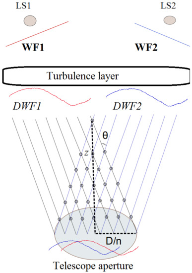
Figure 1.
Slodar geometry of optical beams from two spaced light sources falling on the telescope aperture. D—diameter of the telescope aperture, n—number of subapertures of wavefront Shack–Hartmann sensor laying on diameter, LS1—the first infinitely remote light source, LS2—the second infinitely remote light source, WF1—the plane wavefront from LS1, WF2—the plane wavefront from LS2, DWF1—the wavefront distorted by turbulence layer from LS1, DWF2—the wavefront distorted by turbulence layer from LS2, z—the height of crossed beams, —the angle between LS1 and LS2.
Distorted wavefronts from the infinitely remote light sources are shifted by an amount proportional to the height of the turbulent layer.
The algorithm of the Slodar technique includes the steps [15]:
- (i)
- Continuous registration of short exposure images of at least two spaced light sources (spots) using two Shack–Hartmann wavefront sensors;
- (ii)
- Estimation of local slopes of wavefronts for each subaperture in the two light spot patterns obtained by two sensors;
- (iii)
- Calculations of the time-averaged spatial autocovariance for each source;
- (iv)
- Calculations of cross-correlation coefficients between local slopes of the wavefronts from each light source using the Formula (2) [15]:where —indices of the subapertures, t—time, —local slopes of the wavefront on the subaperture of the first Shack–Hartmann wavefront sensor , —local slopes of the wavefront on the subaperture of the second Shack–Hartmann wavefront sensor , —the number of crossed subapertures;
- (v)
- The turbulence characteristics are estimated using cross-correlation functions and autocovariance function;
- (vi)
- Recovering the profiles of turbulent characteristics up to the maximum height is determined by the geometry of light beams from spaced light sources. Heights of crossing beams is estimated using relation (3) [15]:—zenith angle, —the distance between centers of analyzed subapertures.
The vertical resolution of Slodar method is low fairly. Modern tasks in the physics of the atmosphere, atmospheric optics and adaptive optics including wide field of view systems require higher vertical resolution. We focus on the development of the remote method for atmospheric turbulence profiling.
3. Slodar Based Method with Higher Vertical Resolution
3.1. Proposed Approach to Improvements of Slodar-Based Techniques
We propose a modified statistical method for detection of the atmospheric turbulent layers based on the analysis of wavefront distortions in crossed optical beams. It is known that it is necessary to register wavefront distortions from two or more spaced light sources in Slodar technique. This makes it possible to analyze wavefront distortion in the atmospheric regions in crossing light beams. In comparison with the Slodar technique, the proposed method is based on measurements of wavefront distortions from one object, the spatial position of which changes in time. For example, the daily displacement of the Sun for an observer on the Earth’s surface is equal to 15 arcsec/s. The relative position of the light source (sunspot) on the photosphere during measurements may be considered unchanged.
The geometry of crossing light beams from solar light source falling on the telescope aperture in our method is shown in Figure 2. Since the light source is significantly remote, the wavefront at the upper boundary of the atmosphere can be considered as flat. When radiation propagates in the earth’s atmosphere, the wavefront is distorted due to atmospheric turbulence.
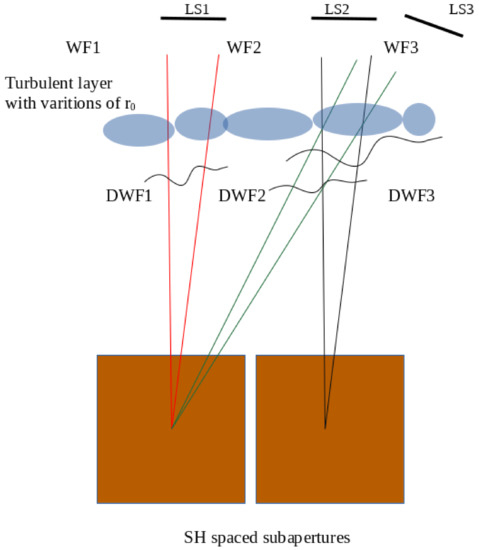
Figure 2.
Geometry of optical beams falling on the telescope aperture in our method. Subapertures are shown by squares. DWFs are the wavefronts distorted by turbulence layer. Atmospheric inhomogeneities are shown by ovals.
Proposed method includes the steps:
- (i)
- Selection of small fragments of the solar image (solar pore or spot). The size of the solar image influences the accuracy of the estimation of gravity center displacements;
- (ii)
- Continuous measurements of short exposure images of single light source (solar pore or spot) using Shack–Hartmann wavefront sensor. To obtain statistically reliable atmospheric characteristics the time series should not be too short;
- (iii)
- Control of frame frequency of the wavefront sensor. It is important due to the fact that the variations of frame frequency at negative air temperatures cause an error in estimation the angle between two beams and, consequently, the heights of the atmospheric layers;
- (iv)
- Estimation of subimage gravity center displacements for each subaperture for different moments of time;
- (v)
- Determination of the time window and the sizes of the light beams shown by red, green and black lines in Figure 2. The time window determines the size of the fragments of time series of the subimage gravity center displacements. We divide measured total time series of the image gravity center displacements in fragments. Each fragment corresponds to the light beam with the known size;
- (vi)
- Estimation of correlation functions between time series fragments of the wavefront slopes at different moments of time. The light beam at the reference subaperture is shown by black lines. The light beam at the spaced subaperture at the subsequent point in time is shown by green lines.
- (vii)
- are indices of the subapertures, t is time, is time shift, are slopes of the wavefront on the subaperture of the Shack–Hartmann wavefront sensor, are slopes of the wavefront on the spaced subaperture , q is the window size, Q is number of time series fragments used, is function filtering small-scale distortions of the wavefront, is the number of the subapertures. If or then distance between centers of subapertures will be equal to:
- (viii)
- Heights of atmospheric layers are determined by Formula (8)where is zenith angle to recalculate distance to the height, is the distance between centers of analyzed subapertures. During the day, the Sun changes its angle in azimuth as well as zenith. Knowing the time between frames , we can determine the angle between light beams at different moments in time.
Averaging for subapertures as well as using a set of reference light beams gives the possibility to obtain the repeatability probability functions of cross-correlation coefficients at different heights. The determination of the mean value of cross-correlation coefficients at the given height allows us to obtain statistically robust estimations.
3.2. Vertical Resolution of Slodar Technique and Proposed Method with Temporal Lag
The main point in the recovering height profiles of the atmospheric turbulence by means of the analysis of the space distribution of the wavefront distortions at the aperture is vertical resolution as well as range of the heights. The vertical resolution in the Slodar technique is limited by the number of the spaced subapertures. Together with that, the vertical resolution in the proposed approach depends on the angle between reference light beam and light beam shifted in time. The vertical resolution of the method is non-uniform, and is changed from 50 m to several hundred meters in free atmosphere. In the atmospheric boundary layer, the step between the nodes is minimal and decreases to 20 m. In our measurements, we used Shack–Hartmann sensors with 8 × 8 or 12 × 12 subapertures installed in the adaptive optics system of the Large solar vacuum telescope. Considering Shack–Hartmann sensors with 8 × 8 and 12 × 12 subapertures, we may obtain the dependencies of the layers heights on the number of subapertures n in the Slodar technique shown in Figure 3a.
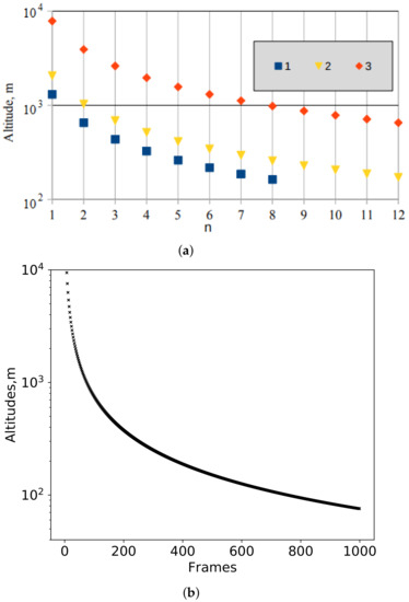
Figure 3.
(a) The dependencies of the layers heights on the number of subapertures n in the Slodar technique. Line 1 corresponds to the 8 × 8 subapertures, line 2 and 3 corresponds to the 12 × 12 subapertures and different angles. (b) The dependencies of the layers heights on the number of frames in the proposed method.
A total number of the atmospheric layers in the Slodar technique is limited by only 8–10. The number of the atmospheric layers for the central reference subaperture is halved (4–5 layers).
Figure 3b shows the dependence of the altitude of the atmospheric layers on the number of frames for the new method, similar to the Slodar technique (8 × 8 subapertures). The total number of atmospheric layers (points) increases by more than an order of magnitude and is ∼200. Analysis of Figure 3a,b shows that the spatial resolution in the modified method is high enough, the highest density of nodes is observed in the lower atmospheric layers.
We have experience in both determining wavefront distortions [22,23] and developing methods for determining vertical profiles [21,24]. The example of the Hartmann pattern obtained at the Large Solar Vacuum Telescope is shown in Figure 4. Main parameters of LSVT and Shack–Hartmann wavefront sensor used are given in Table 1. Measurements of the wavefront have been performed for the time period from 26 June to 28 June 2018.
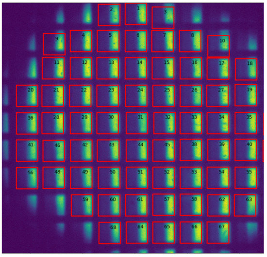
Figure 4.
Hartmann pattern obtained at the Large solar vacuum telescope. Red squares correspond to the subapertures used in calculations.

Table 1.
Main parameters of LSVT and Shack–Hartmann wavefront sensor.
4. Simulation of the Gravity Center Displacements in Shack–Hartman Sensor. The Propagation of the Wavefronts through the Turbulent Layer
We divide the atmosphere in M turbulent layers and each layer has B projected wavefront distortions representing their contribution on the gravity centers displacements measured by the WFS. In the measurements of the wavefront distortions in crossing light beams with temporal lag, it is necessary to take into account the temporal changes of the small-scale wavefront distortions associated with the wind at the different heights.
Let us compare the scales. It is known that the Fried parameter is the characteristic size of small-scale wavefront distortions. Usually, the characteristic values of range from 5 to 10 cm at the wavelength m. Suppose we have time series of the image gravity center displacements measured by Shack–Hartmann sensors with frequency of 300 Hz. Let us analyze the atmospheric turbulent layer at the height of 1 km. Then, the physical size of the region in the atmosphere due to the Sun’s movement (15 arcsec/s) at height of 1 km will be about 0.24 mm/frame. The scale associated with the wind is about 3.3 cm/frame. This means that there are several intersections of the light beams within 10 cm. The obtained estimates of the scales per frame associated with the wind transfer are smaller than the Fried parameter and much smaller than the outer scale of turbulence, which is tens of meters. The proximity of the obtained estimates to the Fried parameter gives us reason to believe that the proposed new approach to the formation of regions with crossing beams can be used in solving the problem of low vertical resolution in the Slodar technique. Using the proposed approach, it is possible to obtain additional nodes in the classical Slodar technique and, thus, the vertical resolution will increase. This effect is especially noticeable for frequencies close to 1 kHz.
Our studies show that the probability of repeatability of the Fried parameter from statistical point of view depends on the low-frequency component of time variations of and on the mean Fried parameter.
We propose the formula for probability distribution function:
where is Gamma function, , , is amplitude, is mean value of . We believe that the optical turbulence in the atmospheric layer obeys this function for large averaging.
To minimize the effect of wind transfer on the analysis of wavefront distortions in crossed light beams, we use the accumulated amplitudes of wavefront distortions (in modulo) for the selected time interval T. It should be noted that the time interval T is selected from the characteristic scale of low-frequency changes in wavefront distortions. The accumulated amplitudes for two crossing light beams are multiplied by each other. For each layer, the array of crossing beams is selected and the function C is averaged. In fact, we are analyzing the response in spaced distortions at the telescope aperture due to the total distortions of the wavefront, the largest contribution to which comes from the low-frequency components. The analysis of the low-frequency components of wavefront distortions is associated with the outer scale of turbulence and makes it possible to identify atmospheric turbulent layers.
The repeatability probability function of the Fried parameter measured by DIMM at the Sayan solar observatory site is shown by blue bars in Figure 5. Red bars correspond to the repeatability probability function of the Fried parameter calculated using Formula (9).
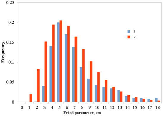
Figure 5.
Repeatability probability function of the Fried parameter measured by DIMM at the Sayan solar observatory site. Line 1 corresponds to the measured values of . Line 2 corresponds to the estimated values of . Mean value of the Fried parameter is equal to 6.3 cm.
Figure 6 shows repeatability probability functions of the Fried parameter for different mean values of .

Figure 6.
Repeatability probability functions of the Fried parameter for different mean values of . Color lines correspond to the different mean values of . Mean value of the Fried parameter is about 6 cm.
Assume the wavefronts propagate through the turbulent layer. Repeatability probability functions correspond to cm and cm (Figure 6). Light beams are crossing at the height of this turbulent layer. Then, the function estimated from the triangulation of local slopes of the wavefronts has shape shown by green line in Figure 7. Red and black lines correspond to the functions estimated for cm and cm, respectively.
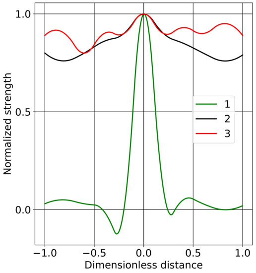
Figure 7.
Estimated correlation functions for one turbulent layer.
5. Conclusions
The Slodar based method with temporal lag to detect the atmospheric turbulent layers using a single Shack–Hartmann wavefront sensor measurements is proposed. The scheme uses the accumulated wavefront distortions registered from solar objects (images of pores or spots) at different points of time. The proximity of the obtained estimates gives reason to believe that the proposed new approach to the formation of regions with crossing beams can be used in solving the problem of low vertical resolution in the Slodar technique. Using the proposed approach, it is possible to obtain additional nodes in the classical Slodar technique and, thus, vertical resolution will increase. This effect will be especially noticeable for frequencies close to 1 kHz. The total number of atmospheric layers (volumes with crossing light beams) increases by more than an order of magnitude and is about 200 for adaptive optics system of the Large Solar Vacuum Telescope. The analysis of the low-frequency components of wavefront distortions is associated with the outer scale of turbulence and makes it possible to identify atmospheric turbulent layers. Analysis of simulated functions shows that the difference between the minimum and maximum of the function is less than for . Nevertheless, the difference reaches 30 % for pronounced turbulent layers. Preliminary data indicate good agreement between the calculation results using the proposed method and lidar observations [25].
Author Contributions
A.Y.S. performed the calculations, developed the method. V.P.L. and P.G.K. formulated solutions to the task, A.V.K., D.Y.K., I.V.R. and M.Y.S. were engaged in the experiments. All authors have read and agreed to the published version of the manuscript.
Funding
This research was predominantly funded by MK-444.2021.4 and RSF grant 19-79-00061. Measurements are partially supported the base financing of FR program II.16 using the Unique Research Facility Large Solar Vacuum Telescope http://ckp-rf.ru/usu/200615/. The work V.P.L. was carried out with funding from the project “Development of methods and systems for adaptive correction for the formation of coherent beams and optical images in the atmosphere”. The work M.Y.S. is supported by State Task of Limnological Institute of the Siberian Branch of the Russian Academy of Science 0345–2019–0008 “Evaluation and prediction of ecological state of Lake Baikal and its surrounding area under the anthropogenic influence and climate change”.
Institutional Review Board Statement
Not applicable.
Informed Consent Statement
Not applicable.
Data Availability Statement
Data are available upon request.
Conflicts of Interest
The authors declare no conflict of interest.
References
- Grigoryev, V.M.; Demidov, M.L.; Kolobov, D.Y.; Pulyaev, V.A.; Skomorovsky, V.I.; Chuprakov, S.A. Project of the Large Solar Telescope with mirror 3 m in diameter. Sol. Terr. Phys. 2020, 6, 14–29. [Google Scholar]
- Shikhovtsev, A.Y.; Kovadlo, P.G.; Kiselev, V.V. Astroclimatic statistics at the Sayan solar observatory. Sol. Terr. Phys. 2020, 6, 102–107. [Google Scholar]
- Kovadlo, P.G.; Shikhovtsev, A.Y.; Lukin, V.P. Development of the Model of Turbulent Atmosphere at the Large Solar Vacuum Telescope Site as Applied to Image Adaptation. Atmos. Ocean. Opt. 2019, 32, 202–206. [Google Scholar] [CrossRef]
- Iersel, M.; Paulson, D.A.; Wu, C.; Ferlic, N.A.; Rzasa, J.R.; Davis, C.C.; Walker, M.; Bowden, M.; Spychalsky, J.; Titus, F. Measuring the turbulence profile in the lower atmospheric boundary layer. Appl. Opt. 2019, 58, 6934–6941. [Google Scholar] [CrossRef]
- Odintsov, S.L.; Gladkikh, V.A.; Kamardin, A.P.; Nevzorova, I.V. Determination of the Structural Characteristic of the Refractive Index of Optical Waves in the Atmospheric Boundary Layer with Remote Acoustic Sounding Facilities. Atmosphere 2019, 10, 711. [Google Scholar] [CrossRef]
- Blary, F.; Ziad, A.; Borgnino, J.; Fantei-Caujolle, Y.; Aristidi, E.; Lanteri, H. Monitoring atmospheric turbulence profiles with high vertical resolution using PML/PBL instrument. SPIE 2014. [Google Scholar] [CrossRef]
- Kellerer, A. Layer-oriented adaptive optics for solar telescopes. Appl. Opt. 2014, 51, 5743–95751. [Google Scholar] [CrossRef]
- Zhang, L.; Guo, Y.; Rao, C. Solar multi-conjugate adaptive optics based on high order ground layer adaptive optics and low order high altitude correction. Appl. Opt. 2017, 25, 4356–4367. [Google Scholar] [CrossRef]
- Zhong, L.; Zhang, L.; Shi, Z.; Tian, Y.; Guo, Y.; Kong, L.; Rao, X.; Bao, H.; Zhu, L.; Rao, C. Wide field-of-view, high-resolution Solar observation in combination with ground layer adaptive optics and speckle imaging. Astron. Astrophys. 2020, 637, A99. [Google Scholar] [CrossRef]
- Shikhovtsev, A.Y.; Kovadlo, P.G.; Kiselev, A.V. The method to restore the profiles of atmospheric turbulence from solar observations. In Proceedings of the SPIE, XXV International Symposium, Atmospheric and Oceanic Optics, Atmospheric Physics, Novosibirsk, Russia, 30 June–5 July 2019; Volume 112081E. [Google Scholar]
- Tokovinin, A.; Kornilov, V. Accurate seeing measurements with MASS and DIMM. Mon. Not. R. Astron. Soc. 2007, 381, 1179–1189. [Google Scholar] [CrossRef]
- Vernin, J.; Roddier, F. Experimental determination of two-dimensional spatiotemporal power spectra of stellar light scintillation Evidence for a multilayer structure of the air turbulence in the upper troposphere. J. Opt. Soc. Am. 1973, 63, 270–273. [Google Scholar] [CrossRef]
- Shepherd, H.W.; Osborn, J.; Wilson, R.W.; Butterley, T.; Avila, R.; Dhillon, V.S.; Morris, T.J. Stereo-SCIDAR: Optical turbulence profiling with high sensitivity using a modified SCIDAR instrument. MNRAS 2014, 437, 3568–3577. [Google Scholar] [CrossRef]
- Wang, Z.; Zhang, L.; Kong, L.; Bao, H.; Guo, Y.; Rao, X.; Zhong, L.; Zhu, L.; Rao, C. A modified S-DIMM+: Applying additional height grids for characterizing daytime seeing profiles. Mon. Not. R. Astron. Soc. 2018, 478, 1459–1467. [Google Scholar] [CrossRef]
- Wilson, R. SLODAR: Measuring optical turbulence altitude with a Shack–Hartmann wavefront sensor. Mon. Not. R. Astron. Soc. 2002, 337, 103–108. [Google Scholar] [CrossRef]
- Butterley, T.; Wilson, R.; Sarazin, M. Determination of the profile of atmospheric optical turbulence strength from SLODAR data. Mon. Not. R. Astron. Soc. 2006, 369, 835–845. [Google Scholar] [CrossRef]
- Wang, L.; Schöck, M.; Chanan, G. Atmospheric turbulence profiling with slodar using multiple adaptive optics wavefront sensors. Appl. Opt. 2008, 47, 1880–1892. [Google Scholar] [CrossRef]
- Wilson, R.; Butterley, T.; Sarazin, M. The Durham/ESO SLODAR optical turbulence profiler. Mon. Not. R. Astron. Soc. 2009, 399, 2129–2138. [Google Scholar] [CrossRef][Green Version]
- Osborn, J.; Wilson, R.; Butterley, T.; Shephard, H.; Sarazin, M. Profiling the surface layer of optical turbulence with SLODAR. Mon. Not. R. Astron. Soc. 2010, 406, 1405–1408. [Google Scholar] [CrossRef]
- Butterley, T.; Osborn, J.; Wilson, R. Error sources in SLODAR turbulence profile fitting. J. Phys. Conf. Ser. 2015, 595, 012006. [Google Scholar] [CrossRef]
- Shikhovtsev, A.; Kovadlo, P.; Lukin, V.; Kiselev, A.; Kolobov, D.; Kopylov, E.; Shikhovtsev, M.; Avdeev, F. Statistics of the Optical Turbulence from the Micrometeorological Measurements at the Baykal Astrophysical Observatory Site. Atmosphere 2019, 10, 661. [Google Scholar] [CrossRef]
- Antoshkin, L.V.; Botygina, N.N.; Bolbasova, L.A.; Emaleev, O.N.; Konyaev, P.A.; Kopylov, E.A.; Kovadlo, P.G.; Kolobov, D.Y.; Kudryashov, A.V.; Lavrinov, V.V.; et al. Adaptive optics system for solar telescope operating under strong atmospheric turbulence. Atmos. Ocean. Opt. 2017, 30, 291–299. [Google Scholar] [CrossRef]
- Lavrinov, V.V.; Lavrinova, L.N. Reconstruction of the wavefront distorted by atmospheric turbulence using a Shack–Hartmann sensor. Comput. Opt. 2019, 43, 586–595. [Google Scholar] [CrossRef]
- Shikhovtsev, A.Y.; Kiselev, A.V.; Kovadlo, P.G.; Kolobov, D.Y.; Lukin, V.P.; Tomin, V.E. Method for Estimating the Altitudes of Atmospheric Layers with Strong Turbulence. Atmos. Ocean. Opt. 2020, 33, 295–301. [Google Scholar] [CrossRef]
- Banakh, V.A.; Smalikho, I.N. Lidar observations of atmospheric internal waves in the boundary layer of the atmosphere on the coast of Lake Baikal. Atmos. Meas. Tech. 2016, 9, 5239–5248. [Google Scholar] [CrossRef]
Publisher’s Note: MDPI stays neutral with regard to jurisdictional claims in published maps and institutional affiliations. |
© 2021 by the authors. Licensee MDPI, Basel, Switzerland. This article is an open access article distributed under the terms and conditions of the Creative Commons Attribution (CC BY) license (http://creativecommons.org/licenses/by/4.0/).