Visibility and Ceiling Nowcasting Using Artificial Intelligence Techniques for Aviation Applications

Abstract

This work presents a novel approach for simulating visibility (Vis) and ceiling base height (H_c) in up to 1 h using several machine learning (ML) algorithms. Ten years of meteorological data at 15 min intervals for Santos Dumont airport (SDA), Rio de Janeiro, Brazil were used in the ML method training and testing process. In the investigation, several categorical and regressive algorithms were trained and tested, and the results were verified with observations. The forecast results reveal that the categorical methods produced satisfactory results only up to 15 min for visibility prediction with the probability of detection greater than 85%. On the other hand, the regressive methods were found to be more capable of generating an accurate prediction of Vis and H_c compared to categorical method up to 60 min. The forecast evaluation metrics for Vis and H_c had correlation coefficients of 0.99 ± 0.00 and 0.96 ± 0.00, with mean absolute errors of 324 ± 77 m, and 167 ± 21 m, respectively. Results suggested that ML methods can improve the prediction of Vis and H_c up to 1 h when accurate observations are used for the analysis.

1. Introduction

Visibility and low ceiling parameters are often a matter of concern in aircraft landing operations because of their obstruction of the pilot’s view over the airport. The Instrument Landing System (ILS), an accurate vertical and lateral landing guiding technology, permits airplanes to land with significantly reduced visibility and ceiling. Despite the fact that many airports have been certified to operate in accordance with instrument flight rules (IFR), some of them lack ILS and must rely on often inaccurate weather forecasts to avoid an unexpected landing impossibility due to visibility or ceiling limitations. According to the Brazilian Aeronautical Information Service (www.aisweb.decea.mil.br, accessed on 15 July 2021), there are 141 airports in Brazil that are approved for IFR operations, although only 47 of them presently have an ILS. Although rain and drizzle may impact the visibility and ceiling height (H_c) significantly, mist and fog are the most restrictive events affecting the mentioned parameters in Brazilian airports [1].

Recently, a review of aviation meteorological issues presented all types of weather events that are critical for aviation operations [2]. It stated that aviation accidents related to Vis and H_c can reach up to about 30%, and come after wind impact.

The genesis of fog/mist in forecast models is usually a significant problem due to poor representation of the microphysical and aerosol properties [2]. For example, an objective 12 h fog prediction model was developed based on the curve adjustment analysis via the least-squares technique of the observational data for Porto Alegre airport [3]; a numerical weather forecasting model for the regional scales was utilized to investigate the evolution of local mesoscale circulation and its impact on the occurrence of night fog formation in São Paulo [4]; and an alternative stochastic model for fog forecasting was established for the Guarulhos International Airport [5]. A visibility forecasting model developed in the early 1980s for fog events at the airports of Curitiba and Porto Alegre concludes that detailed observations and improved physical algorithms are required for accurate Vis predictions [6]. Moreover, investigations [7,8] on the physical and synoptic processes of coastal fog/stratus clouds concluded that they are related to a wave disturbance field in trade winds in northern Brazil and a high-pressure displacement along South America’s east coast in conjunction with a low hot core barotropic occurrence in northern Argentina [9,10] These studies highlighted the difficulty in forecasting the life cycle of marine and coastal fog.

Later in the 2000s, machine learning was limited to a single ML algorithm for visibility and ceiling predictions [11]. A neural network was tested to diagnose Vis using the Met Office’s unified model prediction [12]. This study concludes that the performance of the parameterization is determined by the quality of the meteorological input parameters and the structure of the parameterization. Because of the changing weather conditions over short time periods, weather parameters are critical to improving aviation operations. Then, a pioneering method for very short-term forecasting [13] was developed based on neural network algorithms to predict the Vis and H_c at Guarulhos Airport, São Paulo. Similarly, a fog prediction method based on a ML algorithm was developed for the Brazilian Air Force aerodrome at Pirassununga using meteorological observation data collected from 1989 to 2008, and it was concluded that the suggested neural network algorithm predictions are 95 percent equivalent to observations [14]. A series of works [15,16,17], explored the use of ML algorithms for short-term forecasting of convective events for the Rio de Janeiro metropolitan region. The current results of the ML algorithms show that they are capable of nowcasting convective events with a high probability and low false alarm ratio. Recently, a fog forecasting method based on the ML algorithm was developed for the Afonso Pena International Airport in Paraná, Brazil [18]. The algorithm diagnoses Vis based on 15 min observed and predicted meteorological data, from the automatic surface meteorological station and simulated data using the numerical model of Weather Research and Forecast, respectively. The correlation coefficient of the 24 h forecast, at 15 min intervals, and the observations is close to 90%. The fog predictions are slightly biased, i.e., with a delayed onset and anticipated demise in 30 min or less.

On the other hand, numerical weather prediction (NWP) models perform poorly for low visibility and ceiling predictions [19]. In 2015, an investigation was conducted on the impact of the horizontal resolution of a regional climate model (RCM) on the reproduction of local weather characteristics related to fog in the metropolitan region of São Paulo [20]. RCM simulations showed the ability to characterize fog events with horizontal resolutions of 50 km and 20 km using data from June to September for 2003 and 2004 and stated that increased resolution resulted in prediction improvement of the fog occurrence.

The landing procedure in adverse weather conditions at the SDA in Rio de Janeiro is usually difficult for three reasons: (1) its runways are short; (2) there is no ILS to be used; and (3) its location is very close to the Rio Janeiro-Niterói bridge and Sugarloaf Mountain, as seen in Figure 1a,b. According to the INFRAERO (Airport Management Company, Brasília, Brazil) yearbook [21], approximately 100,144 aircraft landed during 2018, 9,206,059 passengers traveled through the SDA, and it was ranked as the third airport in Brazil that was most impacted by visibility restrictions. The Rio-São Paulo air bridge runs between Santos Dumont and Congonhas Airports, connecting the two largest cities in Brazil and representing 58% of SDA movements, with an average duration of 45 min.

The focus of this research is to use machine-learning-based regressive and categorical algorithms to develop new short-term Vis and H_c forecasts for SDA, with potential general application to other Brazilian airports. In this work, Section 2 provides the location of the project and observations. Section 3 presents the methods and characteristics of the ML algorithms used in the work. Section 4 is for the results. Section 5 is the conclusions derived from this work.

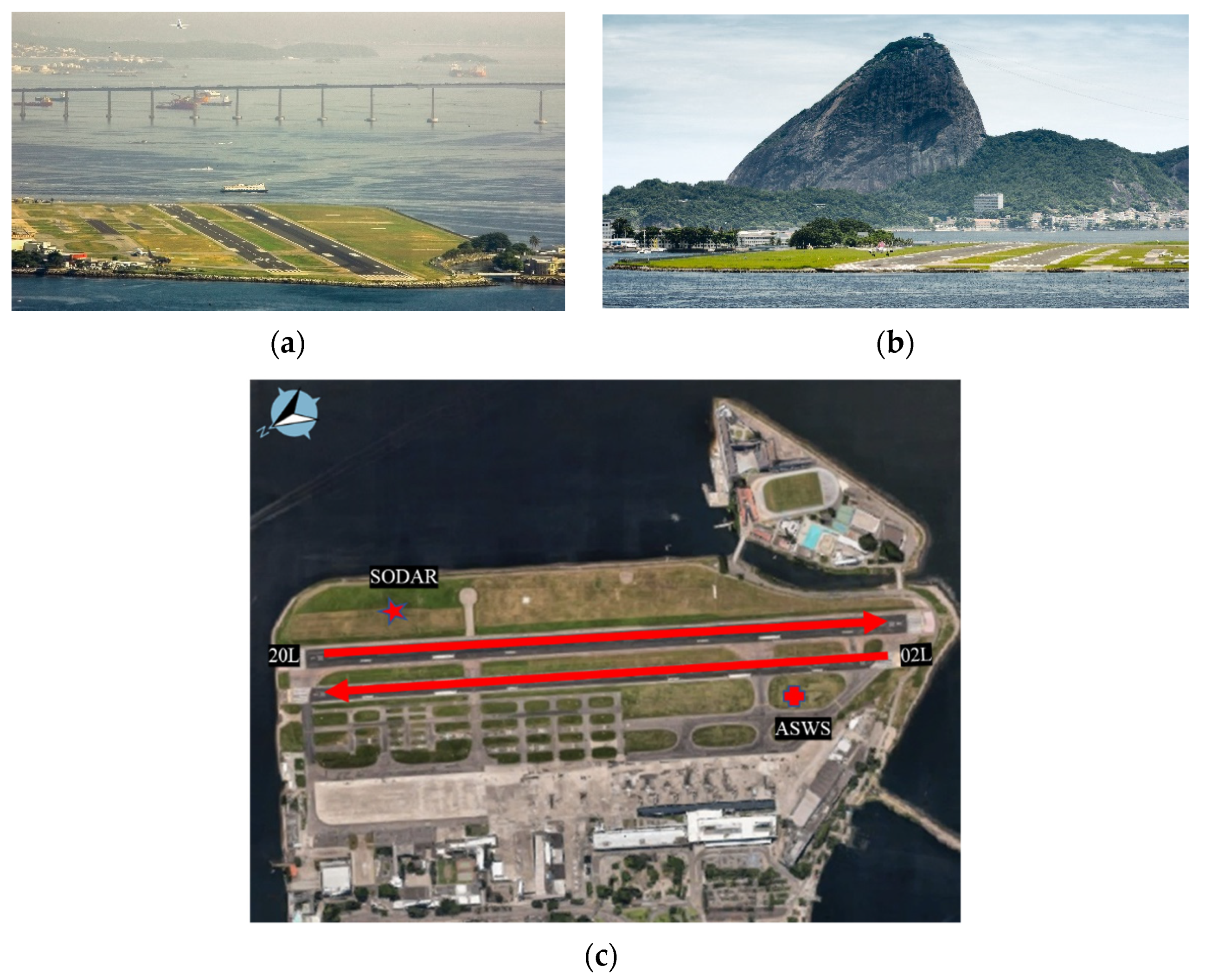
2. Project Site and Observations

The SDA is located at 22.9103° S and 43.1631° W, near the center of Rio de Janeiro. Figure 1 shows the airport views from the northern and southern points. The Sugarloaf Mountain (pique at 407 m) 4000 m away from the two airport runways is shown in Figure 1c. The length of main runway identified as 20L/02R is 1323 m long, and only 63 m longer than the secondary runway (20R/02L).

Considering the aircraft landing restrictions imposed by the obstacles, the Airspace Control Department established the visibility and ceiling limits for landing on the runways.

Table 1. Shows the operational limits for Vis and ceiling representing the three landing procedures on the runways of the SDA.

Landing Procedure	Runway
	20	2
(1) RNAV/GNSS	4500 m/1000 feet	5000 m/1000 feet
(2) NDB	3700 m/1200 feet	4800 m/1500 feet
(3) RNAV/RNP	1600 m/300 feet	1600 m/300 feet

presents the operational limits for visibility (m) and ceiling height (feet) for the three main landing procedures at SDA. These procedures are (1) Area Navigation/Global Navigation Satellite Systems (RNAV/GNSS), (2) Non-Directional Beacon (NDB), and (3) Area Navigation/Required Navigation Performance (RNAV/RNP).

Observations for this work came from three sources: (1) SOnic Detection And Ranging (SODAR) as atmospheric profiler; (2) Automatic Surface Weather Station (ASWS); and (3) human observers.

Table 2. Observation characteristics and meteorological variables used in the machine learning algorithms during training and testing. A total of 253 meteorological variables were used in the analysis.

Source Freq. (min)		(Input) Variable		Variabl qty.	Record qty.	Data Period	Output
		Primary Derived
(1)	15	β (h,−t), where h and t are equal to 30, 40, 50, 60 e 70 m and 0, 15, 30, 45, 60 and 120 min, respectively	u (h,−t), v (h,−t), wa (h,−t), EDR (h,−t) and TKE (h,t), where h and t are equal to 30, 40, 50, 60 e 70 m and 0, 15, 30, 45, 60 and 120 min, respectively	150	70,080	2017 to 2018	Visibility-range-t (where range is equal to 4500, 3700, 1600 m) and/or Ceiling-range-t (being equal to 1000 ft)/cloudquant (okta) for forecast periods (where t is equal to 15, 30, 45 and 60 min).
(2)	15 *	Month, Julian day, year, hour, Ta (h,t), θdir (h,−t), Uh (h,−t), RHw (h,−t), Td (h,−t), Ps (h,t) and RHw (h,t), Hc (t) *, where h and t is equal 2 and 0,15, 30, 45, 60 and 120 min), respectively	-----------	73	350,400	2009 to 2018
(3)	60 **	-----	Vis (−t), Ceiling (−t), Cq (−t), Cc (−t), Clcc (−t), where t is equal to 0, 15, 30, 45, 60 and 120 min	30	87,600	2009 to 2018

* The ceiling height is registered automatically by a ceilometer which is part of the ASWS instrument set. ** For when restriction has occurred.

shows details about the data sources and the 253 meteorological variables labeled as primary (collected directly from the meteorological instruments) and derived (determined using the primary). The parameters used are the predominant visibility (Vis), the ceiling (H_c), cloud cover (C_c), or cloud quantity (C_q), low cloud cover in okta (C_lcc), backscatter intensity (β), surface horizontal wind direction in degrees (θ_dir) and horizontal wind speed (U_h), zonal wind component (u), meridional wind component (v), vertical air velocity (w_a), turbulent kinetic energy in (TKE), energy dissipation rate (EDR), relative humidity to water in % (RH_w), surface atmospheric pressure(P_s), dew point temperature (T_d), and air temperature (T_a). The red star and cross in Figure 1c represent the locations of SODAR and ASWS at SDA, respectively.

3. Method

In this work, machine learning analysis with categorical or regressive algorithms were used to evaluate Vis and H_c predictions at the SDA, because they are commonly used to recognize physical patterns in a specific data set. They are based on the principle that it is possible to learn from a set of training data and consequently be able to correctly classify new standards [22]. This research is part of a sequence of short-term prediction studies based on machine learning algorithms that have been carried out by the Applied Meteorology Laboratory at the Federal University of Rio de Janeiro and can be found in the work of [13,15,16,17,18,23,24]. So, in the present study, the WEKA (Waikato Environment for Knowledge Analysis) software package (version 3.8.4) [25] developed by the University of Waikato in New Zealand was used, with and without the Auto-WEKA subsystem [26,27]. WEKA was chosen because it has a series of machine-learning-based algorithms that can be used to classify thermodynamic atmospheric patterns in the data set related with Vis and H_c limits at the SDA.

3.1. Detailed Analysis

Knowing that meteorological observations represent the variation in time and space of the local atmospheric thermodynamic behavior, local atmospheric patterns with restricted Vis and H_c thresholds for landing procedures were obtained at the above-mentioned airport, following the steps below:

i.

Taking the 15 min ASWS data as a reference, the other data were chronologically disposed, and then their statistical consistency was verified. Data were represented at 15, 30, 45 min for each hour, and all the observations were interpolated to the same time intervals (Table 2). Overall, the number of observations at 15 min intervals reached 350,400 data;

ii.

The history of event occurrences that were limited by the airport operating Vis and H_c threshold values were examined;

iii.

The inputs (the meteorological variables, primary and derived) were selected by measuring the cross-correlation between a given variable and the class (output), and then the redundant ones were eliminated;

iv.

Data sets were generated in order to train and test categorical and regression algorithms. For categorical data sets, the vector input was represented by variables (in columns 2 and 3 of Table 2), that met the intervals of Vis(t) ≤ 4500, 3700, 1600 m, connected to respective outputs associated with the advanced values of Vis(+t) for each prediction time of 15, 30, 45, and 60 min. These inputs were then connected to a binary output (target) of YES or NO, depending on whether the Vis intervals was satisfied. For regressive data sets, the vector inputs (variables) were directly coupled to the Vis(+t) or H_c(+t)/C_q(+t) values of each prediction time of 15, 30, 45, and 60 min (because of the uncertainty in the observation of ceiling data, only regressive algorithms were used for ceiling prediction);

v.

The data sets (categorical and regressive) were then randomly divided into 60% for training and 40% for testing the categorical and regressive algorithms, respectively. This is a frequent practice to avoid overfitting, which occurs when a statistical model fits previously observed data very well but fails to predict new results.

vi.

The YES and NO records of the categorical algorithms training dataset, defined in step v, were balanced through the WEKA ClassBalancer option in four configurations: (1) unmodified data set, (2) 50% YES, and 50% NO, (3) 60% YES and 40% NO, (4) 65% YES and 35% NO for the prediction times using operational thresholds. For regressive algorithms, the training test data sets were defined as in step iv without any artificial adjustment;

vii.

Cross-validation approach (this includes dividing the complete data set into k mutually exclusive subsets of the same size, one for testing and the remaining k-1 for parameter estimation and assessing the algorithm’s accuracy, [28]) was used to train all categorical algorithms available in WEKA, with the four training dataset configurations defined in step vi. Similarly, regressive algorithms were trained. The forecast preliminary findings were examined, and the algorithms with the highest performance (here referred to as selected ones) were chosen for future examination.

viii.

Using the proper test dataset to run the algorithm tests. Section 4.3, Section 4.4, Section 4.5, Section 4.6 discuss the results of the highest performing category and regressive selected algorithms with WEKA’s default configuration.

ix.

Training-test experiments for each prediction time were carried out using the categorical or regressive original data set with Auto-WEKA (version 2.0) [27]. In this tool, all available algorithms were tested and their hyperparameters optimized, which employs the unmodified dataset partitioned into 70% training and 30% testing (thus step iv is ignored here) [26]. Each experiment yielded a rank of the top-performing algorithms from best to worst.

3.2. Algorithm Evaluation

The WEKA software with several classical statistics was used to evaluate the performance of categorical and regressive algorithms. The categorical algorithms have their forecasts versus the observed values by using a two-dimensional contingency table that makes it possible to determine the following categorical statistics [29]: (1) probability of detection (POD) that is a measured fraction of observed events that were correctly predicted—a perfect score is 1; (2) false alarm ratio (FAR), a measure of the fraction of YES predictions in which the event did not occur—a perfect score is 0; (3) BIAS, which measures the proportion of the event frequency prediction by the frequency of the observed events—a perfect score is 1; (4) F-measure (F-M), a measure of the accuracy of a test—a perfect score is 1; and (5) KAPPA, a way of measuring the performance of the binary classification algorithms, where the perfect agreement is 1 [30].

The WEKA software evaluates regressive algorithms that have their performances mainly evaluated by the four following statistics [29]: (1) correlation coefficient (CC), which represents a measure of linear correlation between the forecasts and observations. It varies from +1 and 1, where here values near 1 are desired. (2) Mean absolute error (MAE), which is a measure of error between paired observation and forecasts. The perfect score is zero. (3) Relative absolute error (RAE), expressed as a ratio, comparing the mean residual error to errors produced by a trivial method. The result of a practical method (or its predictions are better than a trivial method) generates a ratio of less than one.

3.3. Characteristics of the Selected ML Algorithms

The statistical evaluation of All WEKA’s algorithms with default configuration given in step vii indicated that the following five algorithms performed better than the others, given as follows:

(1) Bayes Net (BN) is a classifier based on the construction of a Bayesian network, using various research algorithms and quality measures, which provides data structures, network structures, and conditional probability distributions, and can classify binary, class values absent, and nominal classes. [25]. (2) Multilayer Perceptron (MP) consists of standard perceptron with a defined number of hidden units using the activation function (for example, ReLu or sigmoid) and optimization based on minimizing the loss of quadratic error function [25]. (3) Random Forest (RF) is a classifier that consists of a collection of tree classifiers and is trained in different subsets of input resources, and the one with the best performance is chosen [31]. (4) REPTree (RT) is a quick decision tree, which uses the logic of the decision and regression tree and creates several trees in different iterations, selecting the best of all trees generated through the mean square error [25]. Finally, (5) the Hoeffding Tree (HT) consists of a decision tree induction algorithm capable of learning from large data streams, assuming that the distribution generation examples does not change over time, as well as exploring the fact that a small sample may be sufficient to choose an ideal division attribute [25].

4. Results

In this section, results are presented for Vis and H_c predictions using the strategy described in the method section.

4.1. Visibility Thresholds

The data set had occurrences of 11,070, 3996, and 728 low visibility events at 15 min intervals with Vis ≤ 4500, 3700, and 1600 m, respectively. Figure 2 illustrates the hourly (a) and monthly (b) distributions of these events. This reveals that the three main aircraft landing procedures, (1) RNAV/GNSS, (2) NDB and (3) RNAV/RNP (Table 1), were in some ways are compromised by visibility restriction every hour of the day, with a critical period just before sunrise until close to noon (approximately from 06 am to 11 am) throughout all months, and a critical period between May and July.

4.2. Ceiling Thresholds

Similar to Vis analysis, using a ceiling-related threshold, Figure 3 illustrates the hourly (a) and monthly (b) distributions of 4736 events with H_c ≤ 1000 ft from May to July, which is the most critical period. Figure 3b reveals that the RNAV/GNSS (1) landing procedure is affected in some way for the entire day. The critical period usually occurred before sunrise until close to noon (06 a.m.–11 a.m.).

4.3. Algorithm Training and Results

The task of training and testing machine learning algorithms is time-consuming, and success depends directly on the choice of variables (input) that characterize weather hazard conditions, such as the local thermodynamic state of the atmosphere that precedes the occurrence of restrictions on the operational thresholds of Vis and H_c. Table 2 lists the 253 primary and derived meteorological variables as predictors. Thus, disregarding the 150 variables generated by SODAR (data source 1) in method step vi, the cross-correlation of the remaining 103 variables were analyzed and the redundant ones were eliminated, resulting in an input data set consisting of 20 components, namely: month, Julian day, hour, θ_dir (2,0), U_h (2,0), U_h (2,−15), U_h (2,−30), cl(0), C_lcc (0), T_a (2,0), T_d (2,0), RH_w (2,0), P_s (2,0), Vis (0), Vis (−15), Vis (−30), Vis (−45), Vis (−60), and Vis (−120). These were the inputs used in the various training procedures for the Vis and H_c prediction algorithms. For experiments of training algorithms that included data from SODAR, the cross-correlation of the variables was also analyzed.

Several experiments of training and testing via cross-validation for 15-min forecasting of Vis ≤ 4500 m and H_c ≤ 1000 feet were carried out using all available WEKA’s algorithms with the goal of selecting ML WEKA’s algorithms for future investigation (step vii). Following an evaluation of the performance results of the algorithms, the five algorithms in Section 3.2 were selected and discussed further.

4.4. Visibility Categorical Nowcasting

Experiments were carried out in order to assess visibility forecasts, and the following requirements were satisfied, namely: (1) the five categorical WEKA algorithms selected (step viii in the method section); (2) the three visibility thresholds used were Vis ≤ 4500, ≤3700, and ≤1600; (3) the four prediction times had 15 min intervals up to 60 min; and (4) data set configuration was based on SODAR data or not, also using Auto-WEKA support (namely Auto-WEKA default).

Table 3. Statistical test results of 15 min Vis forecasts ≤ 4500 m for the five algorithms (Alg) selected with input from SODAR (source 1), ASWS (source 2) and observer (source 3). The satisfactory algorithm result is in bold.

Alg	Input Data	POD (YES)	1-FAR (YES)	F-M (YES)	BIAS (YES)	POD (NO)	1-FAR (NO)	F-M (NO)	BIAS (NO)	KAPPA	Data Set Configuration
BN	2 and 3	0.83	0.99	0.72	0.77	0.99	0.83	0.99	0.99	0.71	4
MP	2 and 3	0.88	1.00	0.91	1.04	1.00	0.88	1.00	1.00	0.90	1
RF	2 and 3	0.91	1.00	0.91	0.99	1.00	0.91	1.00	1.00	0.91	Auto-WEKA
HT	2 and 3	0.91	1.00	0.91	1.00	1.00	0.91	1.00	1.00	0.91	1
RT	2 and 3	0.89	1.00	0.90	1.03	1.00	0.89	1.00	1.00	0.90	1
RF	1, 2 and 3	0.89	1.00	0.89	1.00	1.00	0.89	1.00	1.00	0.89	Auto-WEKA

,

Table 4. Statistical test results of 15 min Vis forecasts ≤ 3700 m for the five algorithms (Alg) selected with input from SODAR (source 1), ASWS (source 2) and observer (source 3). The satisfactory algorithm result is in bold.

Alg	Input Data	POD (YES)	1-FAR (YES)	F-M (YES)	BIAS (YES)	POD (NO)	1-FAR (NO)	F-M (NO)	BIAS (NO)	KAPPA	Data Set Configuration
BN	2 and 3	0.89	0.97	0.37	0.26	0.97	0.89	0.98	0.97	0.36	1
MP	2 and 3	0.84	1.00	0.88	1.10	1.00	0.84	1.00	1.00	0.88	1
RF	2 and 3	0.88	1.00	0.89	1.01	1.00	0.88	1.00	1.00	0.88	3
HT	2 and 3	0.82	1.00	0.86	1.12	1.00	0.82	1.00	1.00	0.86	1
RT	2 and 3	0.85	1.00	0.89	1.09	1.00	0.85	1.00	1.00	0.88	1
RF	1, 2 and 3	0.85	1.00	0.85	1.00	1.00	0.85	1.00	1.00	0.89	Auto-WEKA

,

Table 5. Statistical test results of 15 min Vis forecasts ≤ 1600 m for the five algorithms (Alg) selected with input from SODAR (source 1), ASWS (source 2) and observer (source 3). The satisfactory algorithm result is in bold.

Alg.	Input Data	POD (YES)	1-FAR (YES)	F-M (YES)	BIAS (YES)	POD (NO)	1-FAR (NO)	F-M (NO)	BIAS (NO)	KAPPA	Data Set Configuration
BN	2 and 3	0.88	0.99	0.43	0.32	0.99	0.88	1.00	0.99	0.42	1
MP	2 and 3	0.68	1.00	0.78	1.34	1.00	0.68	1.00	1.00	0.78	1
RF	2 and 3	0.88	1.00	0.89	1.02	1.00	0.88	1.00	1.00	0.89	Auto-WEKA
HT	2 and 3	0.56	1.00	0.67	1.50	1.00	0.56	1.00	1.00	0.67	1
RT	2 and 3	0.89	1.00	0.89	1.00	1.00	0.89	1.00	1.00	0.89	1
RF	1, 2 and 3	0.89	1.00	0.89	1.00	1.00	0.89	1.00	1.00	0.89	Auto-WEKA

,

Table 6. Statistical test results of 30 min Vis forecasts ≤ 4500 m for the five algorithms (Alg) selected with input from SODAR (source 1), ASWS (source 2) and observer (source 3). The satisfactory algorithm result is in bold.

Alg	Input Data	POD (YES)	1-FAR (YES)	F-M (YES)	BIAS (YES)	POD (NO)	1-FAR (NO)	F-M (NO)	BIAS (NO)	KAPPA	Data Set Configuration
BN	2 and 3	0.84	0.95	0.49	0.42	0.95	0.84	0.97	0.96	0.47	1
MP	2 and 3	0.75	1.00	0.80	1.15	1.00	0.75	0.99	1.00	0.79	1
RF	2 and 3	0.82	0.99	0.81	1.00	0.99	0.82	0.99	1.00	0.81	Auto-WEKA
HT	2 and 3	0.77	0.99	0.79	1.05	0.99	0.77	0.99	1.00	0.78	1
RT	2 and 3	0.74	1.00	0.78	1.12	1.00	0.74	0.99	1.00	0.78	1
RF	1, 2 and 3	0.82	1.00	0.87	1.13	1.00	0.82	1.00	1.00	0.87	Auto-WEKA

,

Table 7. Statistical test results of 30 min Vis forecasts ≤ 3700 m for the five algorithms (Alg) selected with input from SODAR (source 1), ASWS (source 2) and observer (source 3).

Alg	Input Data	POD (YES)	1-FAR (YES)	F-M (YES)	BIAS (YES)	POD (NO)	1-FAR (NO)	F-M (NO)	BIAS (NO)	KAPPA	Data Set Configuration
BN	2 and 3	0.84	0.96	0.30	0.21	0.96	0.84	0.98	0.96	0.28	1
MP	2 and 3	0.61	1.00	0.70	1.39	1.00	0.61	1.00	1.00	0.70	1
RF	2 and 3	0.75	1.00	0.77	1.05	1.00	0.75	1.00	1.00	0.76	4
HT	2 and 3	0.67	0.99	0.61	0.83	0.99	0.67	1.00	1.00	0.60	1
RT	2 and 3	0.64	1.00	0.72	1.27	1.00	0.64	1.00	1.00	0.72	1
RF	1, 2 and 3	0.71	1.00	0.71	1.00	1.00	0.71	1.00	1.00	0.78	Auto-WEKA

and

Table 8. Statistical test results of 30 min Vis forecasts ≤ 1600 m for the five algorithms (Alg) selected with input from SODAR (source 1), ASWS (source 2) and observer (source 3). The satisfactory algorithm result is in bold.

Alg	Input Data	POD (YES)	1-FAR (YES)	F-M (YES)	BIAS (YES)	POD (NO)	1-FAR (NO)	F-M (NO)	BIAS (NO)	KAPPA	Data Set Configuration
BN	2 and 3	0.81	0.99	0.32	0.24	0.99	0.81	1.00	0.99	0.31	1
MP	2 and 3	0.41	1.00	0.56	2.17	1.00	0.41	1.00	1.00	0.55	1
RF	2 and 3	0.73	1.00	0.76	1.11	1.00	0.73	1.00	1.00	0.76	3
HT	2 and 3	0.17	0.94	0.02	0.05	0.94	0.17	0.97	0.94	0.01	3
RT	2 and 3	0.66	0.34	0.76	1.39	1.00	1.00	1.00	1.00	0.76	1
RF	1, 2 and 3	0.88	1.00	0.92	1.10	1.00	0.88	1.00	1.00	0.71	Auto-WEKA

show the best test results of the 15 and 30 min predictions for the three defined visibility thresholds for the five selected algorithms (here called optimal). It is observed that the performance of the forecast decreases as the prediction time increases and the visibility limit decreases. So that all statistics had the unit’s ideal value, 1-FAR was adopted. Here, it was defined as whether a given method (the latter being defined as the trained and tested algorithms) had satisfactory performance to predict visibility for a given prediction time when their POD and 1-FAR values were ≥0.8. Table 3, Table 4 and Table 5 highlights the statistical results of the 15 min forecast (and those satisfactory algorithms in bold) for visibility thresholds, and reveals that eleven algorithms performed coherently, since the averages of the categorical statistics were almost close to the perfect score (value in parentheses), which were: POD (Y, N) (0.884 ± 0.012, 0.999 ± 0.000), 1-FAR (Y, N) (0.996 ± 0.005, 0.884 ± 0.012), F-M (Y, N) (0.891 ± 0.011, 0.998 ± 0.001), BIAS (Y, N) (1.016 ± 0.022, 1.000 ± 0.000), KAPPA (0.89 ± 0.008).

As previously analyzed, Table 6, Table 7 and Table 8 also shows the best performance algorithms (and those satisfactory algorithms in bold), by visibility limit and 30 min forecast. It is observed that no algorithm obtained a POD (V) greater than 80% for the limit of Vis ≤ 3700 m, and there are only three algorithms, i.e., one and two for Vis ≤ 4500 and Vis ≤ 1600, respectively, with satisfactory performance. The evaluation statistics suffered a percentage reduction (in parentheses) in relation to the 15 min predictions, as follows: POD (S, N) (7.53%, 0.08%), 1-FAR (S, N) (0.08%, 7.53%), F-M (S, N) (5.28%, 0.14%), BIAS (S, N) (5.06%, 0.06%), KAPPA (S, N) (10.89%, 0.008%). The results of the 45 and 60 min forecasts deteriorated significantly, and are therefore not discussed.

4.5. Visibility Regressive Nowcasting

Similar to the previous case, the new experiments were run employing regressive algorithms while considering conditions, as follows: (1) the five selected WEKA regressive algorithms; (2) the three visibility thresholds used Vis = 4500, =3700, and =1600 with four prediction times of 15 min intervals up to 60 min; and (3) two data sets with or without SODAR data, and using Auto-WEKA support.

Table 9. Better statistical results of short-term visibility forecast using regressive algorithms and those whose training was performed using the data set with configuration (5), whose records were divided as Auto-WEKA default.

Algorithm	Prediction Time (min)	Input Data Source	CC	MAE (m)	RAE
RF	15	1, 2 and 3	0.99	198.58	0.04
RF	15	2 and 3	0.99	189.85	0.04
RF	30	1, 2 and 3	0.99	304.86	0.06
RF	30	2 and 3	0.99	291.38	0.06
RF	45	1, 2 and 3	0.99	378.70	0.08
RF	45	2 and 3	0.99	351.85	0.07
RF	60	1, 2 and 3	0.99	409.32	0.08
RF	60	2 and 3	0.99	343.88	0.07

shows a summary of the best statistical results for the test experiments with regressive algorithms for all prediction times, and it is noted that RF is the algorithm with the best performance regardless of the input data set or the prediction time considered. All predictions almost perfectly correlated (column 4), which means that the trends of the predicted values follow the behavior of the observations almost perfectly. Figure 4 shows the three thresholds (±MAE) of visibility represented by the black lines and their respective minimum (cross) and maximum (black triangle) errors for better 15, 30, 45, 60 min predictions. Independent of prediction time, variations in visibility predictions for 4500, 3700, and 1600 m fit into the following ranges (with percentage visibility changes in parentheses): 4148–4852 m (7.8%), 3348–4052 m (9.5%), and 1248–1952 m (22%), respectively. In short, assuming acceptable error in forecasting of the visibility is about 20%, the results of the predictions with the regressive algorithms were more representative than categorical ones. This is verified using the observations.

Figure 5 exemplifies the performance of the set of predictions and observations for a low-visibility event that occurred between 5 a.m. and 1 p.m. on 23 June 2009. Regardless of the forecast time, it is noted that the 15, 30, 45 and 60 min visibility forecasts followed the behavior of the observation (black line in Figure 5) with all correlation coefficients >0.95 and their mean absolute errors ≤ 321 m. This can be verified through the behavior of the predicted visibilities, as they followed the observations almost perfectly; that is, they decreased at 5:45 a.m., remained relatively stable after 8:00 a.m.—when the observed visibility oscillated close to 1000 m—and increased with the increase in observations from 11:45 a.m. Furthermore, the 15, 30, 45, and 60 min forecasts slightly overestimated the observations (based on the mean error of forecast–observation values for each prediction time) by about 146.4, 121.9, 224.2, and 292.1 m, respectively.

4.6. Ceiling Nowcasting

Before presenting the results for forecasting the ceiling and the quantity of clouds, it is important to mention that the SODAR data was collected in the period 2017–2018, and during this period, the ceilometer used, part of the ASWS platform, was inoperative. Thus, training of the algorithms for the ceiling is limited to the 2009–2016 period, and

Table 10. Better statistical results of short-term H_c/C_q forecast using regressive algorithms, whose training was performed using the data set with configuration (5), whose records were divided as Auto-WEKA default.

Algorithm	Prediction Time (min)	Input Data Source	CC	MAE (ft/okta)	RAE
RF	15	2 and 3	0.97	126.13 feet	0.1
RF	15	2 and 3	0.86	0.55 okta	0.32
RF	30	2 and 3	0.97	166.02 feet	0.14
RF	30	2 and 3	0.81	0.69 okta	0.4
RF	45	2 and 3	0.96	182.95 feet	0.15
RF	45	2 and 3	0.83	0.63 okta	0.37
RF	60	2 and 3	0.96	195.19 feet	0.16
RF	60	2 and 3	0.77	0.77 okta	0.44

is missing data from SODAR. Table 6 shows a summary of the best results for the ceiling test experiments with regressive algorithms for all prediction times. Similar to the visibility results, the RF algorithm also results in the best performance of ceiling forecasts, regardless of the input data set or the prediction time considered. It is also found that the predicted values of H_c/C_q of 15, 30, 45 and 60 min are highly correlated with the observations, with their values varying in the range of 0.96–0.97 and 0.77–0.86, respectively (column 4, Table 10), and the observations are found to be close to the predictions, since the MAE and the RAE for ceiling vary in the ranges from 126.13 to 195.19 ft and 0.10 to 0.16 ft, respectively. The results of the three ceiling thresholds (i.e., 1200, 1000, and 300 ft) can be considered encouraging since they vary approximately within the H_c ranges from 1005 to 1395 ft, 805 to 1195 ft, and 105 to 495 ft, respectively.

5. Conclusions

This study proposes a set of objective methods based on ML (using the trained and tested algorithms), with an extremely low computational cost capable of making short-term forecasts of Vis and Hc up to 60 min.

Analysis of historical meteorological data suggested that the weather conditions at any airport can be more impacted by the restriction of visibility than the ceiling, and the critical period of the day is just before sunrise until close to noon during May, June, and July. The results with optimal categorical methods of visibility predictions are satisfactory in 15 min and have not been successful in any forecast for the ceiling. On the other hand, ceiling and visibility predictions based on regressive methods of up to 60 min are encouraging, since the values of the metrics with relatively lower biases are quite acceptable.

In summary, following conclusions can be drawn from the present work:

• ML algorithms resulted in up to 20% better prediction in Vis when regressive techniques were used with a significant amount of reliable data;
• Training data sets need to be improved accurately in temporal and 16 spatial resolutions, and use of data from sensors (visibility meters, ceilometer, etc.) instead of human observations. When sensor observations were used in training, ML algorithms had more accurate Vis and H_c predictions;
• The 1 h Vis and H_c data obtained by observers may not follow the dynamics of some meteorological phenomena, impairing the assertiveness of the method. Furthermore, observations provide a spatial resolution for Vis, which may reduce the efficacy of the algorithm’s training compared to continuous sensor based Vis data. It is obvious that the lack of lengthier history series in the SODAR data profiles, the absence of visibility sensor usage, and the ceilometer’s inoperability since 2016 were all factors that led to the trained algorithm’s performance decline; and
• The ML methods proposed here can identify visibility and ceiling restrictions accurately, thus, they can improve the short-term forecasts of up to 1 h. Thus, the new ML-based methods can be considered an alternative to operational forecasts based on NWP models.

In the future, we intend to use a NWP model to simulate the atmospheric conditions of visibility and ceiling that limits the airport operation, and apply the training and testing of the ML algorithms. Using simulated data and observations, including a long time series of high-frequency data based on SODAR, ceilometer, and automatic weather stations, we will be able to extend the prediction time of visibility and ceiling beyond the one-hour prediction time.

References

- DECEA. Relatório de Performance do Sistema de Controle do Espaço Aéreo Brasileiro (SISCEAB). 2018. Available online: http://especiais.decea.gov.br/performance/wp-content/uploads/2020/08/Rela_SISCEAB_ESTUDO-2_compressed.pdf (accessed on 4 January 2021).
- Gultepe, I.; Sharman, R.; Williams, P.D.; Zhou, B.; Ellrod, G.; Minnis, P.; Trier, S.; Griffin, S.; Yum, S.S.; Gharabaghi, B.; et al. A review of high impact weather for aviation meteorology. Pure Appl. Geophys. 2019, 176, 1869–1921. [Google Scholar] [CrossRef]
- Lima, J.S. Previsão de ocorrências de nevoeiros em Porto Alegre: Método objetivo, São José dos Campos: Instituto de Proteção ao Voo do Ministério da Aeronáutica. Tech. Rep. 1982, 18. [Google Scholar]
- Dias, M.A.F.S.; Machado, A.J. The role of local circulations in summertime convective development and nocturnal fog in São Paulo, Brazil. Bound.-Layer Meteorol. 1997, 82, 135–157. [Google Scholar] [CrossRef]
- Oliveira, G.A. Método Estatístico no Auxílio à Previsão de Nevoeiro Para o Aeroporto de Guarulhos. Master’s Thesis, Federal University of Santa Catarina, Florianópolis, Brazil, 2002. Available online: https://repositorio.ufsc.br/xmlui/bitstream/handle/123456789/83415/188292.pdf?sequence=1&isAllowed=y (accessed on 4 January 2021).
- França, V.D.J. Avaliação da Metodologia de Previsão de Nevoeiro e Visibilidade Horizontal do Modelo ETA. Master’s Thesis, National Institute for Space Research, São José do Campos, Brazil, 2008; p. 172. [Google Scholar]
- Fedorova, N.; Levit, V.; Fedorov, D. Fog and stratus formation on the coast of Brazil. Atmos. Res. 2008, 87, 268–278. [Google Scholar] [CrossRef]
- Fedorova, N.; Levit, V.; Silva, A.O.; Santos, D.M.B. Low Visibility formation and forecasting on the northern coast of Brazil. Pure Appl. Geophys. 2013, 170, 689–709. [Google Scholar] [CrossRef]
- Gultepe, I.; Tardif, R.; Michaelides, S.C.; Cermak, J.; Bott, A.; Bendix, J.; Müller, M.D.; Pagowski, M.; Hansen, B.; Ellrod, G.; et al. Fog research: A review of past achievements and future perspectives. J. Pure Appl. Geophys. 2007, 164, 1121–1159. [Google Scholar] [CrossRef]
- Gultepe, I.; Pagowski, M.; Reid, J. Using surface data to validate a satellite based fog detection scheme. J. Weather. Forecast. 2007, 22, 444–456. [Google Scholar] [CrossRef]
- Hansen, B. A fuzzy logic-based analog forecasting system for ceiling and visibility. Weather Forecast. 2007, 22, 1319–1330. [Google Scholar] [CrossRef]
- Claxton, B.M. Using a neural network to benchmark a diagnostic parameterization: The Met Office’s visibility scheme. Q. J. R. Meteorol. Soc. 2008, 134, 1527–1537. [Google Scholar] [CrossRef]
- Almeida, M.V. Aplicação de Técnicas de Redes Neurais Artificiais na Previsão de Curtíssimo Prazo da Visibilidade e Teto Para o Aeroporto de Guarulhos–SP. Ph.D. Thesis, Federal University of Rio de Janeiro, Rio de Janeiro, Brazil, 2009. Available online: http://www.coc.ufrj.br/pt/teses-de-doutorado/153-2009/1186-manoel-valdonel-de-almeida (accessed on 4 January 2021).
- Colabone, R.O.; Ferrari, A.L.; Vecchia., F.A.S.; Tech, A.R.B. Application of artificial neural networks for fog forecast. J. Aerosp. Technol. Manag. 2015, 7, 240–246. [Google Scholar] [CrossRef]
- França, G.B.; Almeida, M.V.; Bonnet, S.M.; Neto, F.L.A. Nowcasting model of low wind profile based on neural network using SODAR data at Guarulhos airport. Int. J. Remote Sens. 2018, 39, 2506–2517. [Google Scholar] [CrossRef]
- Freitas, J.H.V.; França, G.B.; Menezes, W.F. Convection forecasting using decision tree in Rio de Janeiro metropolitan area. Anuário IGEO 2018, 42, 127–134. [Google Scholar] [CrossRef]
- Almeida, V.A.; França, G.B.; Velho, H.F.C. Short-range forecasting system for meteorological convective events in Rio de Janeiro using remote sensing of atmospheric discharges. Int. J. Remote Sens. 2020, 41, 4372–4388. [Google Scholar] [CrossRef]
- Platenik, J.E.G.; França, G.B.; Neto, A.V.P.; da Silva, R.M.; de Almeida, V.A. Previsão de Nevoeiro Utilizando Multicritérios Baseados em Simulações do Modelo WRF para o Aeroporto Internacional Afonso Pena. Anuário IGEO 2020, 43, 376–383. [Google Scholar] [CrossRef]
- Zhou, B.; Du, J.; Gultepe, I.; Dimego, G. Forecast of Low Visibility and Fog from NCEP: Current Status and Efforts. Pure Appl. Geophys. 2012, 169, 895–909. [Google Scholar] [CrossRef]
- Da Rocha, R.P.; Gonçalves, F.L.T.; Segalin, B. Fog Events and local atmospheric features simulated by regional climate model for the metropolitan area of São Paulo, Brazil. Atmos. Res. 2015, 151, 176–188. [Google Scholar] [CrossRef]
- Perini, A.B.; Filho, D.P.P.; Rodrigues, E.S.; Amaral, F.S.; Reichert, R.F.L. Anuário Estatístico Operacional 2018. INFRAERO. 2019. Available online: https://www4.infraero.gov.br/media/677124/anuario_2018.pdf (accessed on 4 January 2021).
- Bishop, C.M. Pattern Recognition and Machine Learning; Springer: Berlin/Heidelberg, Germany, 2006; ISBN 978-0-387-31073-2. [Google Scholar]
- Silva, W.L.; Neto, F.L.A.; França, G.B.; Matschinske, M.R. Conceptual model for runway change procedure in Guarulhos International Airport based on SODAR data. Aeronaut. J. 2016, 120, 725–734. [Google Scholar] [CrossRef][Green Version]
- Almeida, V.A.; França, G.B.; Velho, H.F.C. Data assimilation for nowcasting in the terminal area of Rio de Janeiro. Ciência Nat. 2020, 42, e40. [Google Scholar] [CrossRef]
- Witten, I.H.; Frank, E.; Hall, M.A.; Pal, C.J. Data Mining: Practical Machine Learning Tools and Techniques, 4th ed.; Morgan Kaufmann: Sydney, Australia, 2016; ISBN 978-0-12-804291-5. [Google Scholar]
- Thornton, C.; Hutter, F.; Hoos, H.H.; Leyton-Brown, K. Auto-WEKA: Combined selection and hyperparameter optimization of classification algorithms. In Proceedings of the 19th ACM SIGKDD International Conference on Knowledge Discovery and Data Mining—KDD ’13, Chicago, IL, USA, 11–14 August 2013; pp. 847–855. [Google Scholar] [CrossRef]
- Kotthof, L.; Thornton, C.; Hoos, H.H.; Hutter, F.; Leyton-Brown, K. Auto-WEKA 2.0: Automatic model selection and hyperparameter optimization in WEKA. J. Mach. Learn. Res. 2016, 17, 1–5. [Google Scholar]
- Holmes, G.; Donkin, A.; Witten, I.H. WEKA: A machine learning workbench. In Proceedings of the ANZIIS ‘94-Australian New Zealand Intelligent Information Systems Conference, Brisbane, Australia, 29 November–2 December 1994; pp. 357–361. [Google Scholar] [CrossRef]
- Wilks, D.S. Statistical Methods in the Atmospheric Sciences, 2nd ed.; Academic Press: London, UK, 2006. [Google Scholar]
- Landis, J.R.; Koch, G.G. The Measurement of Observer Agreement for Categorical Data. Biometrics 1977, 33, 159–174. [Google Scholar] [CrossRef]
- Breiman, L. Random Forests. Mach. Lang. 2001, 45, 5–32. [Google Scholar] [CrossRef]