Thundercloud Electrostatic Field Measurements during the Inflight EXAEDRE Campaign and during Lightning Strike to the Aircraft

Abstract

The AMPERA (Atmospheric Measurement of Potential and ElectRic field on Aircraft) electric field network was integrated on the Falcon 20 (F20) of SAFIRE (the French facility for airborne research) in the framework of EXAEDRE (EXploiting new Atmospheric Electricity Data for Research and the Environment) project. From September 2018, an in-flight campaign was performed over Corsica (France) to investigate the electrical activity in thunderstorms. During this campaign, eight scientific flights were done inside or in the vicinity of a thunderstorm. The purpose of this paper is to present the AMPERA system and the atmospheric electrostatic field recorded during the flights, and particularly during the pass inside electrified clouds, in which the aircraft was struck by lightning. The highest value of atmospheric electrostatic field recorded during these flights was around 79 kV·m⁻¹ at 8400 m of altitude. A normalization of these fields is done by computing the reduced atmospheric electrostatic field to take into account the altitude effect (ratio between the atmospheric electrostatic field and the air density). Most of the significant values of reduced atmospheric electrostatic field magnitude retrieved during this campaign occur between around 5.5 and 9.5 km and are included between 50 and 100 kV·m⁻¹. The highest value measured of the reduced atmospheric electrostatic field is 194 kV·m⁻¹ during the lightning strike of the F20. The merging of these results with data from former campaigns suggests that there is a threshold (depending of the aircraft size) for the striking of an aircraft.

1. Introduction

In the 1980s, flight campaigns have been performed to understand the physical processes occurring during a lightning strike to an aircraft when it flies in areas where the atmospheric electrostatic field generated by the thundercloud is high. This field was measured by an electric field mills network on the skin of the aircraft, and its value just before a lightning strike to the aircraft was recorded. During the C160 campaign performed in the 1980s [1,2], six values of atmospheric electrostatic field were recorded and are associated with a triggered lightning.

A new version of this electric field mills network, called AMPERA (Atmospheric Measurement of Potential and ElectRic field on Aircraft), has been developed by ONERA (Office National d’Etudes et de Recherches Aérospatiales) since 2010. In September 2018, an in-flight campaign was performed over Corsica (France) in the framework of the EXAEDRE (EXploiting new Atmospheric Electricity Data for Research and the Environment) project to investigate the electrical activity in thunderstorms. During this campaign, eight scientific flights were done with a Falcon 20 (F20) of SAFIRE (the French facility for airborne research) inside or in the vicinity of thunderstorms. During the flight of the 8 of October 2018, the aircraft was struck by lightning at an altitude of 8400 m.

The purpose of this paper is to present the AMPERA system and the atmospheric electrostatic field recorded during EXAEDRE flights and then discuss a method to compare the atmospheric electrostatic field values measured by C160 and F20 during lightning strikes.

2. AMPERA System

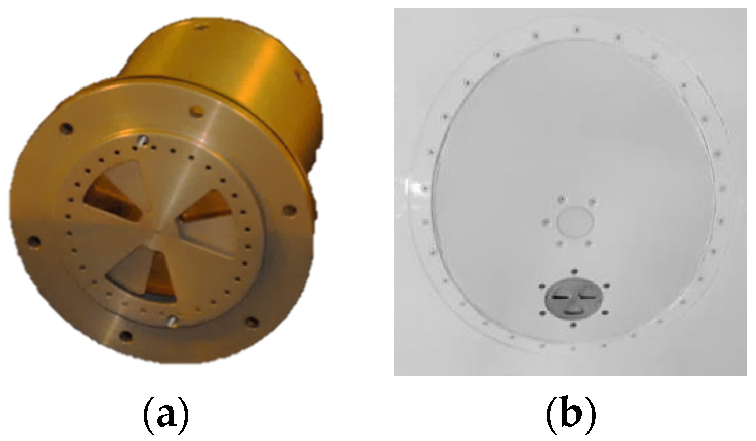
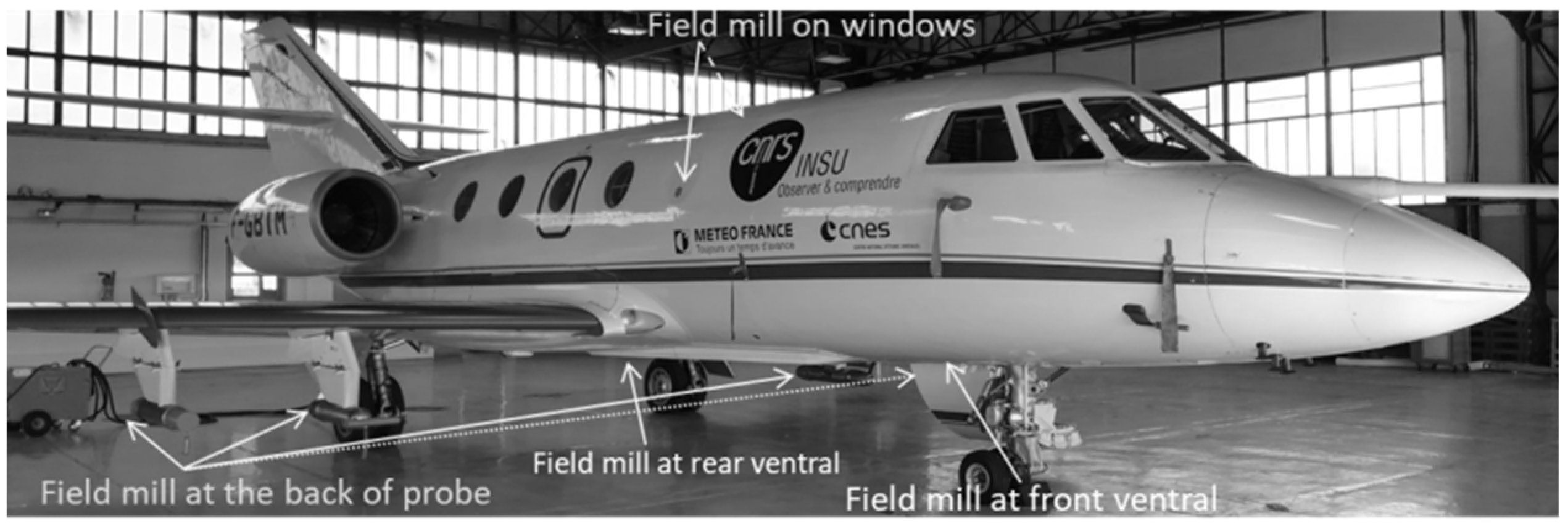
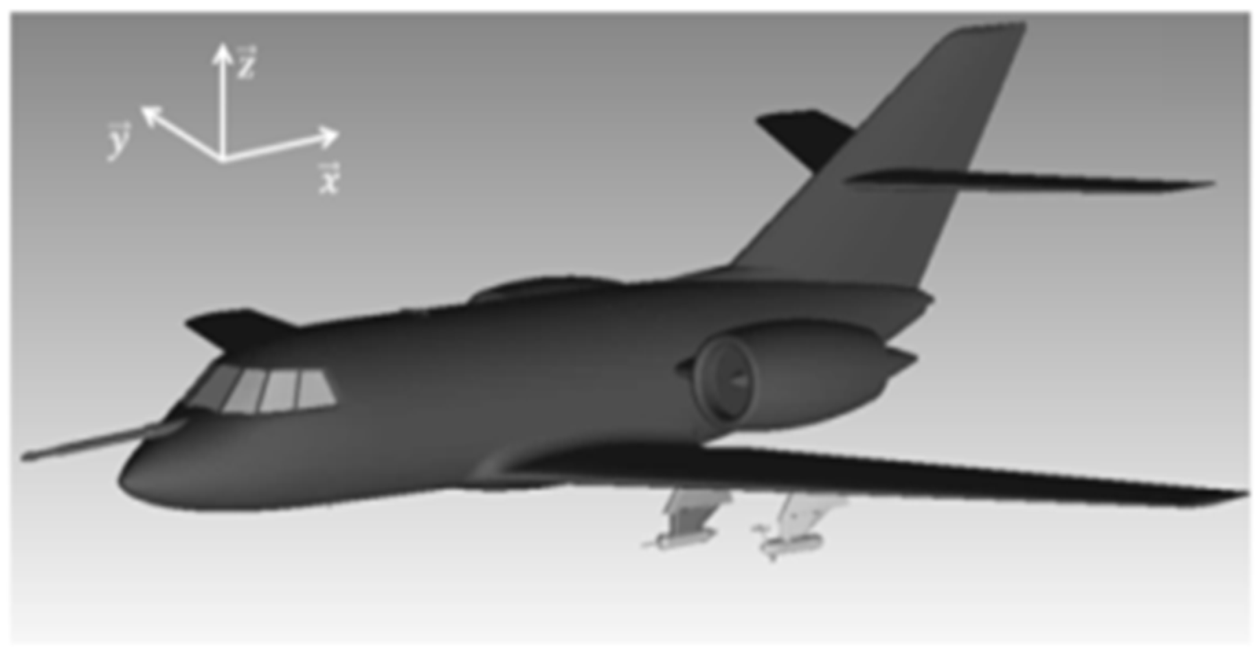
2.1. Electric Field Mill Network on Falcon 20

Since the 1940s, there have been many studies estimating the atmospheric electrostatic field in fair weather conditions as well as in the vicinity of and inside thunderstorms. In this framework, different kinds of sensors have been developed. There are some different techniques to measure the atmospheric electrostatic field [3,4]. Many studies have used different kinds of sensors, for example, the cylindrical field mills [5], the rotating field mills ([6] on airborne, [7] on balloon), the balloon-borne field meters [8,9,10], airborne field meters e.g., [11], or the rocket-borne sensors [12]. From this perspective, airborne field mills have been adopted for atmospheric research by ONERA for decades [13] and tested on different kinds of aircraft (e.g., C160 Transall [1]; Gloster Meteor NF11 [14]; Falcon 20, nowadays).

The AMPERA network implemented on the Falcon aircraft for the EXAEDRE campaign is the same that the one used during the HAIC (High Altitude Ice Crystals) campaign [15]. An illustration of the field mill used is shown in Figure 1a. The characteristics and performance of the sensor, determined from laboratory tests, are detailed in

Table 1. Performance and characteristics of field mill of the AMPERA system.

Physical	Mass	0.870 kg
	Power	28 V (DC); 25 W max
	Size	120 mm × 115 mm
Dynamic Range		+/−5 V/m to +/−1 MV/m
Threshold of Detection	Below 5 kV/m	5 V/m
	Above 5 kV/m	20 V/m
Sampling Rate		10 Hz

. The field mill measures positive values of the electric field when the electric field direction at the field mill head is outwards.

The integration of the eight field mills on the F20 was done by the SAFIRE team (

Table 2. Name and location of the field mills installed on the F20.

Name	Number	Aircraft Location
P1	EFM1	Back of the external left pod
P2	EFM2	Back of the internal left pod
LW	EFM3	Left window (1st left window)
RW	EFM4	Right window (1st right window)
P5	EFM5	Back of the internal right pod
P6	EFM6	Back of the external right pod
FV	EFM7	Front ventral
RV	EFM8	Rear ventral

). Two field mills were installed on the first two windows of the cabin (cf. Figure 1b). Four were integrated to the back of the pods. These locations enable having three couples of sensors, which are symmetrically placed from the fuselage. The two last ones are installed on ventral traps of the fuselage, one at the front and one at the rear (Figure 2).

The field mills P1, P2, P5, and P6 are installed either on the rear of the probes (P2, P5, P6) or on the rear on the fastening system (P1). Unfortunately, a detailed meshing of the fastening system for P1 and P6 was not available, leading to a rough approximation of the P1 and P6 coefficients of Equation (1) (see below). The analysis of the flights has shown that the sensors P1 (EFM1) and P6 (EFM6) cannot be used during the campaign and are removed from the inverse method. So, the analysis has been performed by using six sensors.

2.2. Inverse Method

Based on the assumption of a uniform atmospheric electrostatic field around the aircraft [6,13,16,17,18], the electric field on the aircraft skin can be expressed by the following linear relationship:

$${\mathrm{E}}_{\mathrm{mi}}={\mathsf{\alpha }}_{\mathrm{i}}{\mathrm{E}}_{\mathrm{ox}}+{\mathsf{\beta }}_{\mathrm{i}}{\mathrm{E}}_{\mathrm{oy}}+{\mathsf{\gamma }}_{\mathrm{i}}{\mathrm{E}}_{\mathrm{oz}}+{\mathsf{\lambda }}_{\mathrm{i}}{\mathrm{V}}_{\mathrm{a}},$$

(1)

where E_mi is the electric field recorded by the field mill n°i; E_mi is an electric field perpendicular to the aircraft skin; E_ox, E_oy, and E_oz are the three components of the atmospheric electrostatic field in the aircraft reference (cf. Figure 3); V_a is the aircraft potential; it is associated with the net electrical charge on the aircraft. The electrical charge and the potential are linked by the capacitance of the aircraft; α_i, β_i, λ_i, and γ_i are constant coefficients. Note that these coefficients can be positive or negative except for the λ_i coefficients, which have all the same sign. This is shown by Figure 4a, which plots the electric field measured on the aircraft skin when there is only potential. The figure shows that the electric field variations are similar (in the same direction and with a same feature) from one field mill to another. Figure 4b illustrates the field orientation when the aircraft potential is negative in fair weather where the atmospheric electrostatic field can be neglected.

Figure 5a shows an event where the aircraft is electrically polarized by a mainly vertical atmospheric electrostatic field. In this case, field mills on windows measure negative values until the others placed under the aircraft wings and fuselage measure positive values. Figure 5b shows the effect of the direction of the atmospheric electrostatic field $\overrightarrow{{\mathrm{E}}_0}$ on the electric field at the aircraft skin.

The atmospheric electrostatic field components and the electric potential of the aircraft are computed from:

$$\left[\begin{array}{c}{\mathrm{E}}_{\mathrm{ox}}\\ {\mathrm{E}}_{\mathrm{oy}}\\ \begin{array}{c}{\mathrm{E}}_{\mathrm{oz}}\\ {\mathrm{V}}_{\mathrm{a}}\end{array}\end{array}\right]={\mathrm{A}}^{\mathrm{T}}{\left(\mathrm{A}.{\mathrm{A}}^{\mathrm{T}}\right)}^{-1}\left[\begin{array}{c}\begin{array}{c}{\mathrm{E}}_{\mathrm{m}1}\\ ⋮\end{array}\\ {\mathrm{E}}_{\mathrm{m}6}\end{array}\right],$$

(2)

where $\mathrm{A}=\left(\begin{array}{ccc}{\mathsf{\alpha }}_1& \cdots & {\mathsf{\lambda }}_1\\ ⋮& \ddots & ⋮\\ {\mathsf{\alpha }}_6& \cdots & {\mathsf{\lambda }}_6\end{array}\right)$.

In the EXAEDRE campaign, the A matrix coefficients have been derived in two steps. In the first step, a Poisson equation solver has been used to numerically compute the value of E_mi based on the three-dimensional shape model (cf. Figure 3) of the Falcon 20 aircraft. Note that the geometry and the associated meshing is an approximation of the real aircraft. From a real geometry of the F20, we add the probes and their fastening systems (which are complex 3D objects).

In a second step, the computed coefficients have been corrected using in-flight measurements. During the take-off and initial climb phase, the sensors measure large values mainly due to the electric charging of the aircraft due to the engines (${\mathrm{E}}_{\mathrm{mi}}~{\mathsf{\lambda }}_{\mathrm{i}}{\mathrm{V}}_{\mathrm{a}}$). These measurements have been used to tune the potential coefficients as follows:

• The field mill on the right window (RW, EFM4) is chosen as the reference because it is in a low curvature part of the aircraft where the geometric approximation is small;
• The ratio between the electric field measured $\frac{{\mathrm{E}}_{\mathrm{mi}}}{{\mathrm{E}}_{\mathrm{m}4}}$ has been computed;
• The coefficients of potential are corrected by using the following expression: ${\mathsf{\lambda }}_{\mathrm{i}}=\frac{{\mathrm{E}}_{\mathrm{mi}}}{{\mathrm{E}}_{\mathrm{m}4}}{\mathsf{\lambda }}_4$ where ${\mathsf{\lambda }}_4$ is the potential coefficient associated with the field mill of the right window.

The methods proposed by Winn [19], Koshak [17], and Bateman et al. [20] were not applied because calibration flights have been done either in cloudy conditions where the atmospheric electrostatic field is unknown or at too high altitude where it is too weak to be used. So, no correction has been applied on coefficients associated with the components of the atmospheric electrostatic field. The matrix A obtained after the calibration for the EXAEDRE campaign is shown in

Table 3. Matrix A after the calibration method.

Name	Number	Eox	Eoy	Eoz	Va
P2	EFM2	1.23	3.45	−5.26	0.55
LW	EFM3	2.00	1.41	0.70	0.24
RW	EFM4	2.00	−1.14	0.70	0.24
P5	EFM5	1.23	−3.45	−5.26	0.55
FV	EFM7	2.79	0	−2.06	0.29
RV	EFM8	0.1	0	−1.65	0.19

.

Mach [21] has shown that when an aircraft flies inside thunderclouds, there are some nonlinear terms to add to Equation (1). We assume that these nonlinear terms are associated with the charging of the aircraft’s painted layers due to a part of the triboelectricity effects associated with charge exchanges during impingements of the ice particles with the painted layer. Indeed, most of the charge due to triboelectricity goes to the aircraft grounding, and a small part remains locally stored on the dielectric painted layer, cockpit windows, and radome. This stored charge is caught on the surface and typically relaxed to the aircraft grounding with a decay time of several minutes. We choose to eliminate this nonlinear effect with a first-order high-pass filter with a cut-off frequency equivalent to 5 min applied on the electric field measurements E_mi. During 5 min, the aircraft has flown a distance of about 60 km. By applying this filter, we remove the offset component due to the charge stored on the dielectric painted layer that we observe when the aircraft exits the cloud. The objective of this filter is not to filter the electric field component during pass inside a cloud (around few minutes duration) but to reset the offset before a new pass inside a cloud.

2.3. Inverse Method Error Analysis

Mazur et al. [22] and Mach et al. [23] have shown that there are different sources of error associated with the methodology used. The accuracy is dependent on two causes: the A coefficient matrix that reflects the airplane form factor, i.e., the link between ambient and local field, and the measurement of the electrostatic field on the aircraft surface.

The total error on the evaluation of the aircraft potential V_a and each component of the atmospheric electrostatic field are computed by considering a random error on each measurement (E_mi) and on each computed element of the matrix A. Despite a careful sensor calibration in laboratory and on the aircraft, we consider an overall relative error in the measurement of 1%. For the matrix coefficient, A, the considered error was +/−5%. The errors depend on the electrical state of the atmosphere (E_ox, E_oy, and E_oz) and the relative magnitude of the aircraft potential. The relative error computation has been calculated with an atmospheric electrostatic field of 1 V·m⁻¹ in the aircraft reference by considering the six electric field mills in the EXAEDRE configuration. Each component of the atmospheric electrostatic field is fixed to 1 V·m⁻¹. For this state of the atmosphere, the relative error on each electrostatic field component, on the aircraft potential, and on the magnitude of the atmospheric electrostatic field has been estimated for different values of aircraft potential.

With this theoretical evaluation, we obtain an error on the evaluation of each component around 10 to 13% for the AMPERA system configuration used during the EXAEDRE campaign. For the SAFIRE Falcon 20 in EXAEDRE, due to this error, the minimum detectable atmospheric electrostatic field is about 1000 V·m⁻¹ when the aircraft potential has a magnitude of 100 kV. This finding is not harmful in the context of the atmospheric electrostatic field assessment in thunderstorms because the expected values are higher than this threshold. However, it makes the calibration difficult with maneuvers in fair weather, knowing that the potential values in these cases for the SAFIRE Falcon 20 usually reach 40 kV; that is to say, a minimum detectable atmospheric electrostatic field is 400 V·m⁻¹, which is higher than the fair weather electrostatic field ranges between some. If the aircraft potential is 0 V, we are able to detect an atmospheric electrostatic field of about 10 V·m^-1.

The estimation of the theoretical error is based on the ratio between the aircraft potential and the atmospheric electrostatic field magnitude. This ratio has been computed for all the EXAEDRE campaign flights where the magnitude of the electrostatic field was higher than 6 kV·m⁻¹. This threshold is based on the maximum aircraft potential value measured during the campaign.

Figure 6 represents the normalized cumulative distribution of these ratios for the whole of flights in the cases where the atmospheric electrostatic field magnitude was higher than 6 kV·m⁻¹. For 90% of the cases, the ratio between the aircraft potential and the magnitude of the atmospheric electrostatic field is weaker than 10, which corresponds to a maximum global error on each component between +/−5 and +/−8% for the six-sensor configuration. In the case of the atmospheric electrostatic field magnitude, this corresponds to a maximum global error of +/−4%. This global error remains below +/−5% until the aircraft potential is 25 times higher than the atmospheric electrostatic field magnitude, which covers the majority of cases (around 99%) encountered during the campaign (Figure 6).

3. Atmospheric Electrostatic Field Measurements

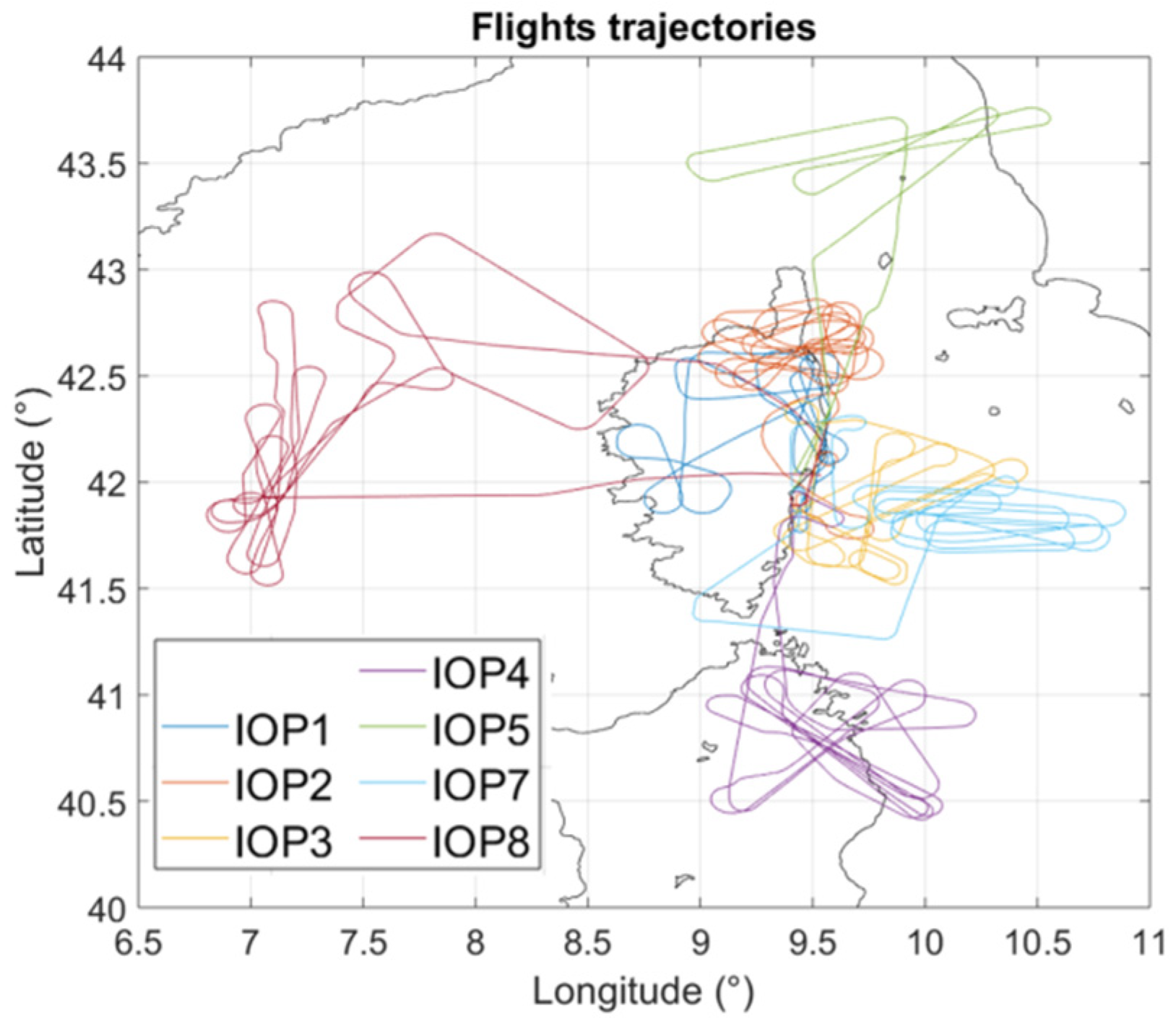
3.1. EXAEDRE Campaign

The EXAEDRE (EXploiting new Atmospheric Electricity Data for Research and the Environment) project (https://www.hymex.org/exaedre/ accessed on 2 December 2021) aims to investigate the electrical activity in thunderstorms. The Special Observation Period (SOP) of this in-flight campaign was performed over Corsica (France) in September and October 2018. This project includes a part of ground instrumentation, as the site of San Giuliano (INRA: Institut National de la Recherche Agronomique) in Corsica, and an airborne component composed by the SAFIRE Falcon 20, on which several sensors have been integrated: four microphysical probes (a Cloud Droplet Probe (CDP-2, [24]), a 2D-Stereo probe (2D-S, [25]), a Precipitation Imaging Probe (PIP, [24]), and a Cloud Particle Imager (CPI, [26])) operated by the French Laboratoire de Météorologie Physique (LaMP), the 95-GHz Doppler Radar System Airborne (RASTA) cloud radar [27,28] and the AMPERA network.

The analysis of the comparison and the combination of the dataset from different instruments will be done in future communication. This paper is only focused on the in-flight electric field measurements.

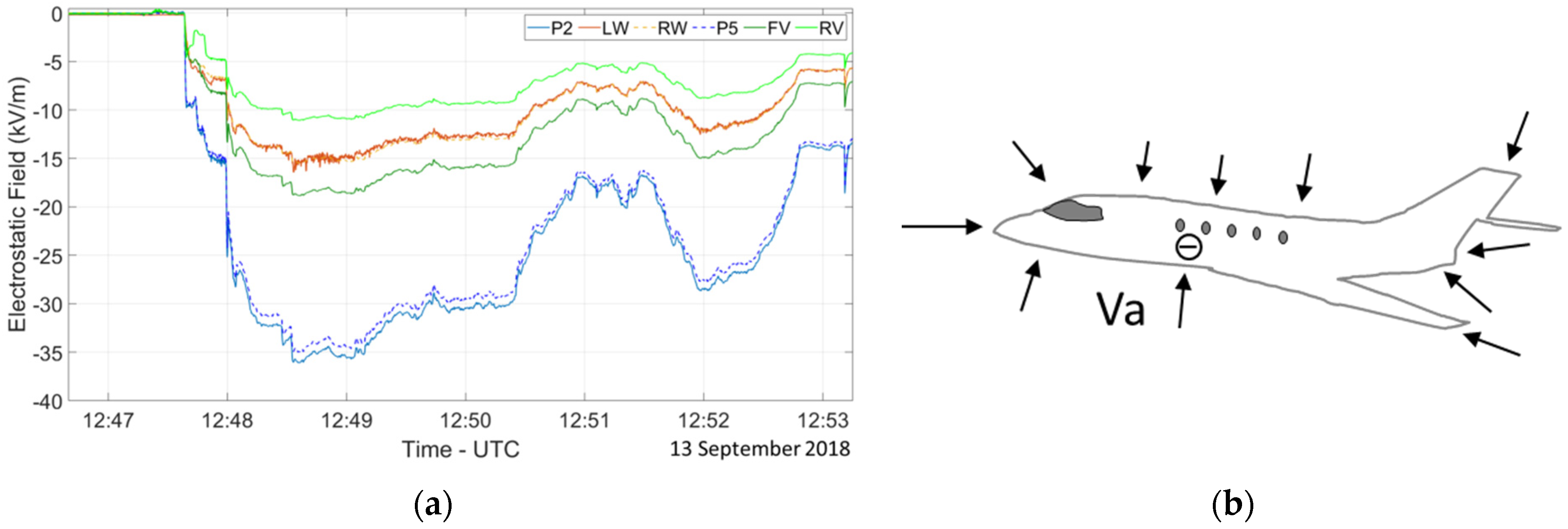
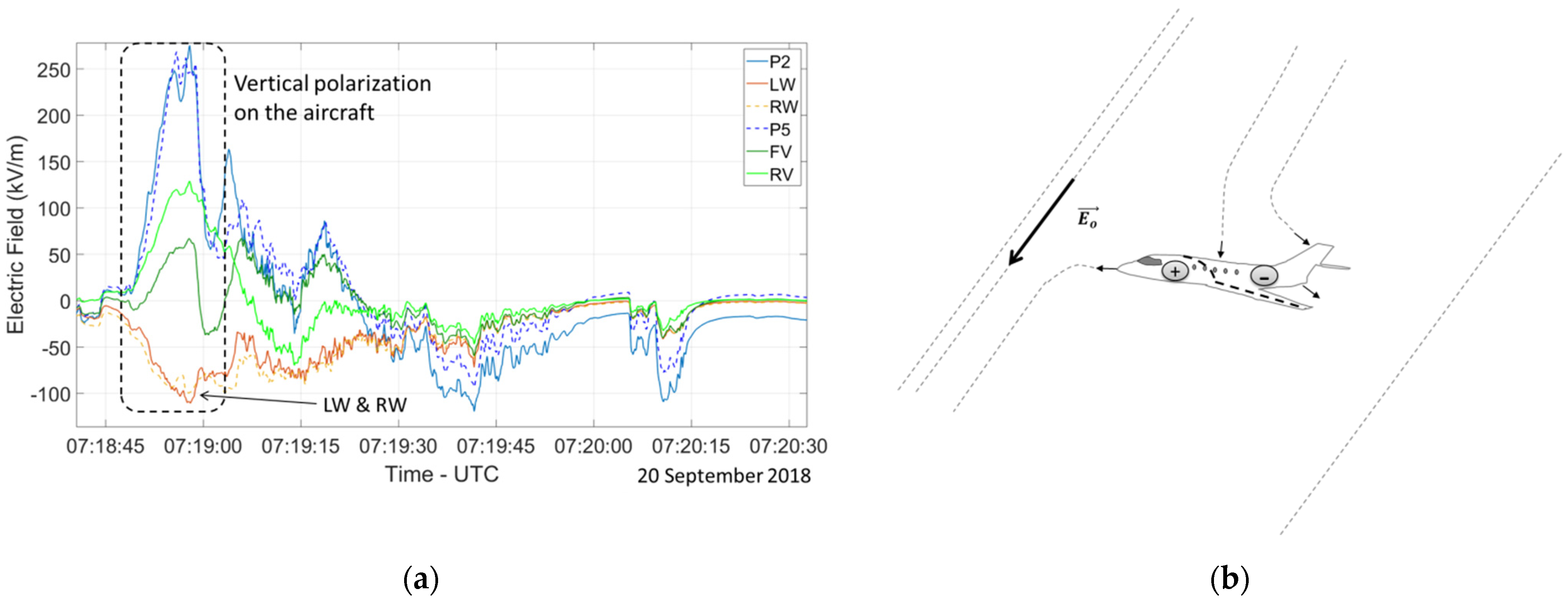
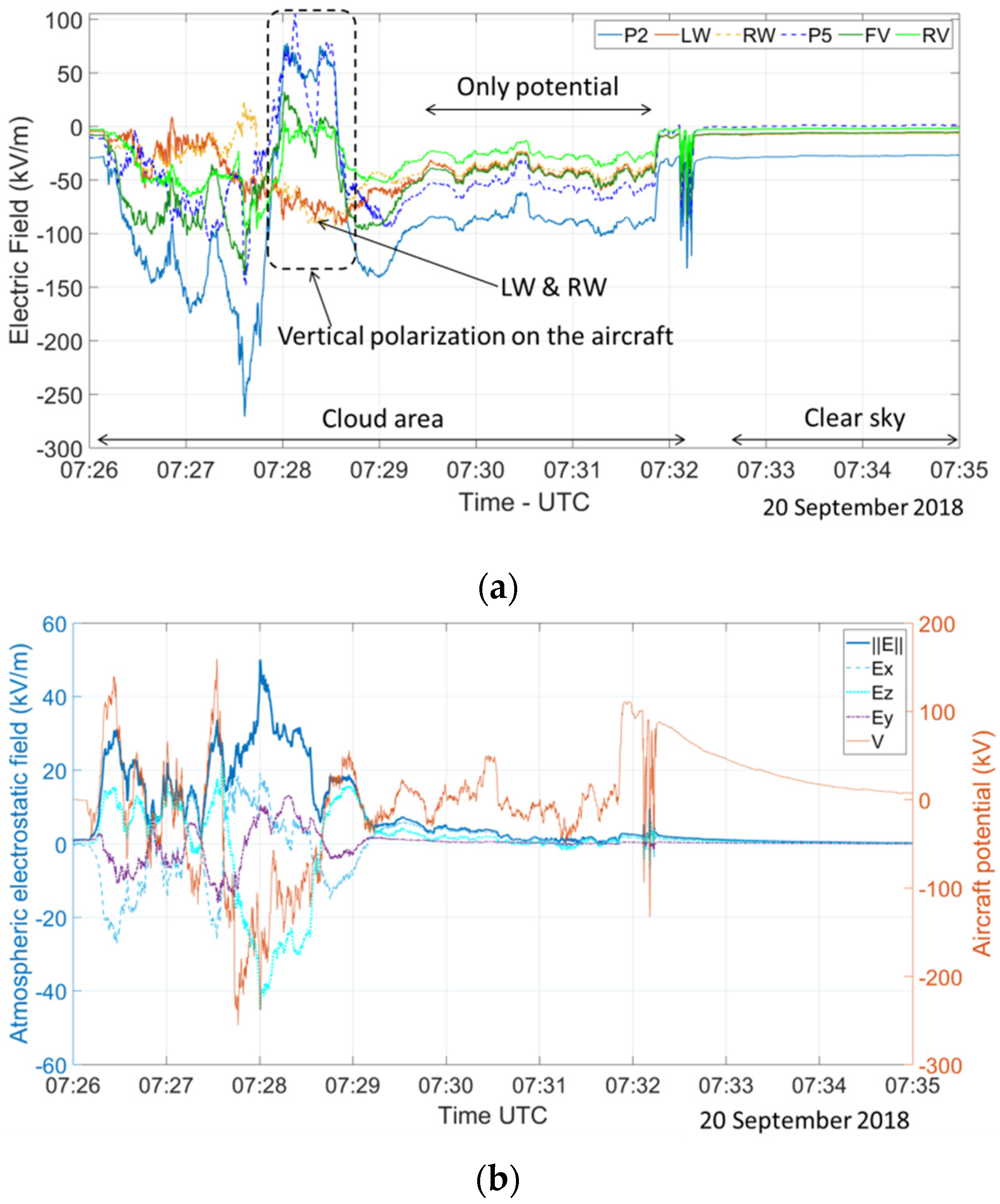
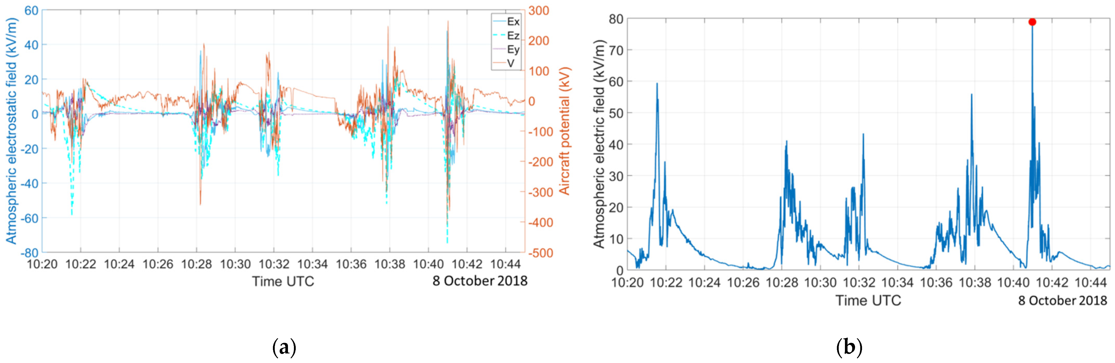
3.2. Electric Field Measurement during EXAEDRE Campaign

Eight scientific flights were performed during the SOP (Special Observation Period) of this campaign to investigate different convective systems in particular by describing legs inside the clouds at different altitude. The flight starts generally at high altitude around 8000 or 9000 m; then, the altitude is decreased with passes around 6000 m and 4500 m. Longitude, latitude, and altitude (and other aircraft parameters such as pitch or roll) are synchronized with the AMPERA measurement. During the flight 6 (IOP 6), several sensors have too noisy measurements to be used as input of the inverse method. The trajectories of the seven flights investigated are presented in Figure 7.

AMPERA is able to measure and retrieve the atmospheric electrostatic field, particularly during periods with strong atmospheric electrostatic field identifiable by a strong electric polarization of the aircraft on the field mill measurements. In flight IOP 4, the time variations of field mill value are shown in Figure 8. In this figure, the entry and the exit of the cloud are shown. During this flight, the northeast of the Sardinia Island is explored to catch moderate convective cells developing in a west flow.

At the beginning of the cloud phase, multiple electric polarizations of the aircraft occur, horizontal and vertical. Around 07:28 UTC, we observe a vertical electric polarization of the aircraft. The electric fields measured by the field mills on the fuselage windows (LW, RW) decrease and become negative while on the other field mills increase to positive value. After 07:29 UTC, the electric fields measured by all the field mills are negative and have similar variations. This indicates that the field mill values are driven by the aircraft potential variation. Just before 07:33 UTC, the aircraft leaves the cloud and flies in clear air, which is visible on the measurement. The inverse method was used to compute the atmospheric electrostatic field and the aircraft potential. At the time corresponding to the maximum electric polarization of the aircraft, the atmospheric electrostatic field reaches 35 kV·m⁻¹ and is mainly vertical. In the second part of the cloud where only potential is measured, the atmospheric electrostatic field magnitude is between 0.5 and 2 kV·m⁻¹. Outside the cloud, the magnitude of the electrostatic field is very weak around 40 V·m⁻¹. This low value can be resolved because the aircraft potential for this case is also very weak around 0 kV after 07:33 UTC.

Other examples are shown in Figure 9 for two crossings of cloudy regions during the flight IOP 8, with different electric polarizations of the aircraft. The conditions of this flight are an upper-level flow low moving to the northeast of Spain, which lead to the development of convective cells southeast of the Corsica Island in southwest flow. The upper part of the figure represents the electric field measurements from the six field mills used to retrieve the atmospheric electrostatic field and its components. The bottom part represents the magnitude of the atmospheric electrostatic field, its components, and the aircraft potential derived from the field mills measurements. In both cases, the vertical electric polarization of the aircraft is shown by the field mills measurements. In both cases, the atmospheric electrostatic field is mainly vertical (high values of E_oz compared to E_ox and E_oy).

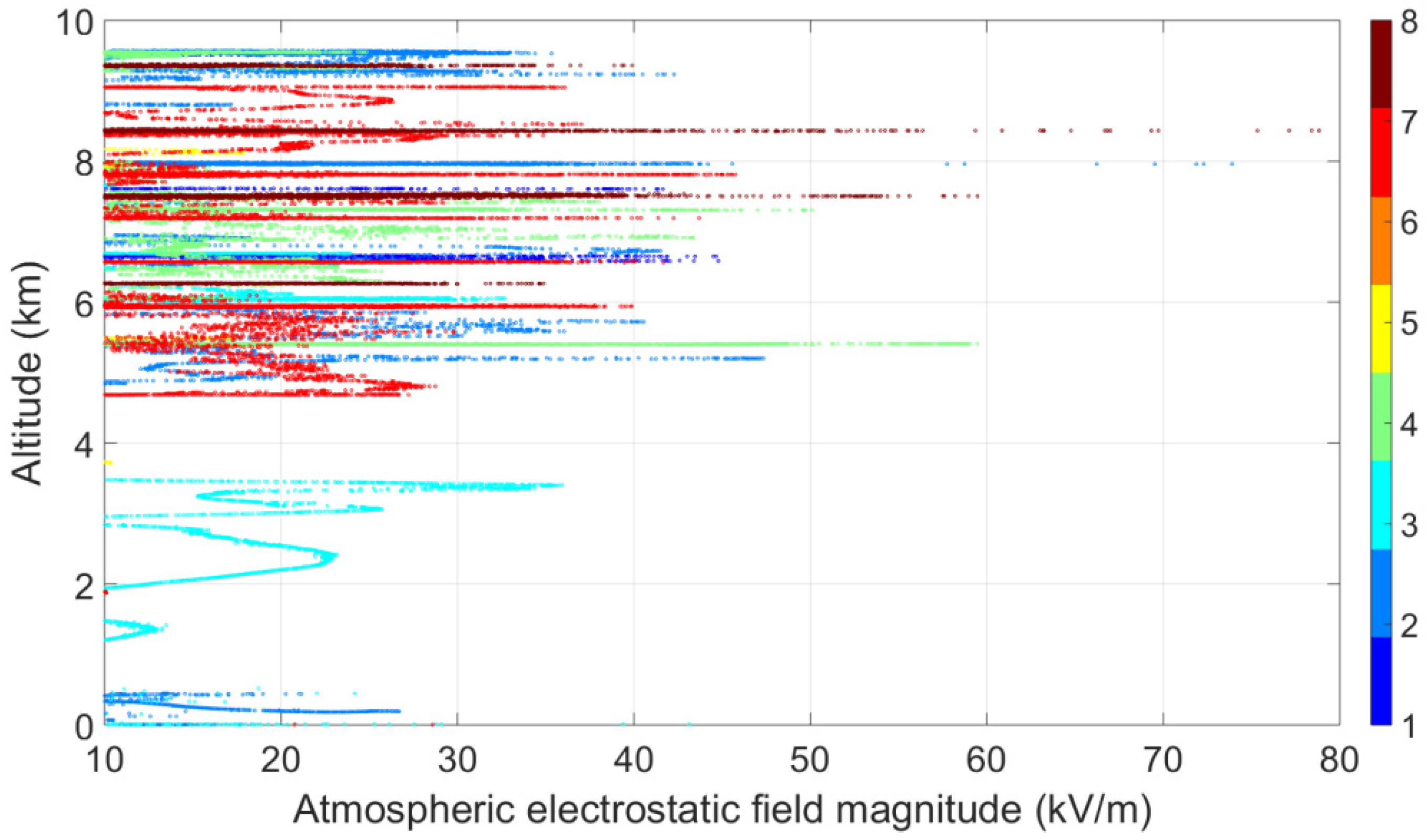
3.3. Magnitude of Atmospheric Electrostatic Field Retrieved during the EXAEDRE Campaign

Dye and Bansemer [29] considered that an atmospheric electrostatic field is strong inside a cloud as soon as it is higher than 10 kV·m⁻¹. This value is consistent with the AMPERA sensitivity, so we focus on these values for the next analysis. Figure 10 shows the values of the atmospheric electrostatic field magnitude for the seven IOP flights versus the altitude. Only values higher than 10 kV·m⁻¹ are plotted. The highest value is 79 kV·m⁻¹ and was measured during flight IOP 8 when the aircraft was struck by the lightning flash. It can be noted that the range of the aircraft potential values corresponding to these values of atmospheric electrostatic field magnitudes (higher than 10 kV·m⁻¹) spread from 0.6 to 432 kV. The extrema are −432 kV and 325 kV. The atmospheric electrostatic field of 79 kV·m⁻¹ associated with the lightning strike to aircraft is coherent with former measurements (realized with balloons [30,31]).

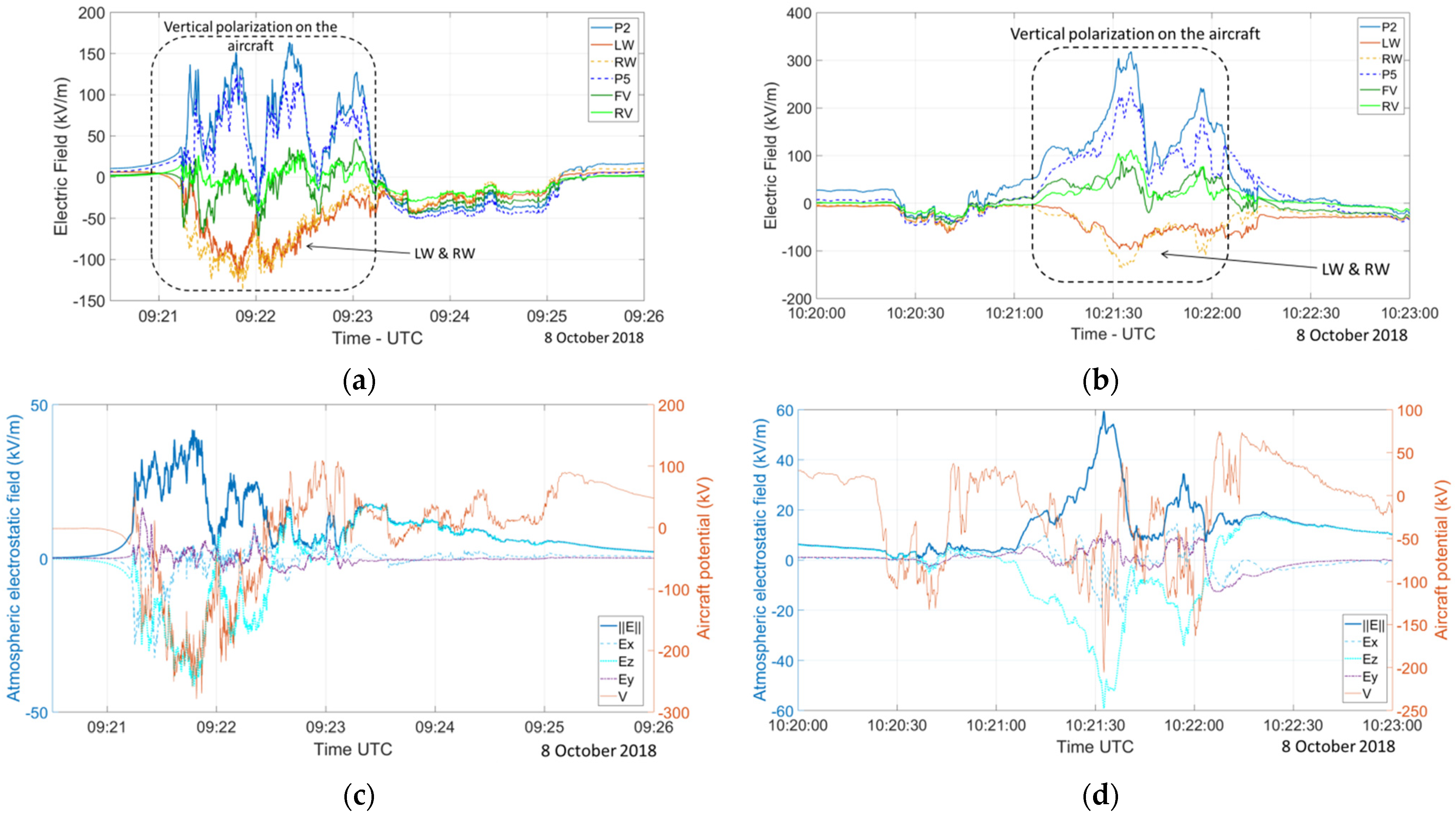
4. Atmospheric Electrostatic Field Measurements

In this part, the analysis is focused on flight IOP 8 during which the lightning struck the aircraft. The aircraft flew inside and near isolated convective areas by describing some loops. During the measuring phase of the flight, the altitude of the aircraft was from 6000 to 10,000 m. At 10 h 40′59″ GMT, the aircraft was struck by lightning (the lightning flash attached on the boom of the F20), and the crew had to stop the flight. The lightning occurred when the aircraft was at 8400 m near a convective zone.

Figure 11a shows the time variation of the electric field measured by each electric field mill for the last 20 min before the lightning strike. The field mills measured the electric field from −140 to 410 kV·m⁻¹. The duration can be split into five main sequences associated with a penetration of the aircraft inside the cloud (cf. Figure 11a, sequences are the periods between the arrows). The period during which the electric field measured by the sensors is low corresponds to the flight track mainly outside or near the cloud except for the second point. In Figure 11b, 2 min around the lightning strike are plotted. At 10 h 40′30”, the measurements show that there is a vertical polarization of the aircraft. The electric fields measured by the field mills on the fuselage windows (LW, RW) become negative, while on the other field mills, they are positive.

The inverse method has been applied to these five sequences. Figure 12a shows that the main component of the atmospheric electrostatic field is vertical (downward) and that the absolute maximum value of this component is 75 kV·m⁻¹. The aircraft potential reaches a maximum of −400 kV. It decreases a few seconds later to −159 kV just before the lightning strike. Figure 12b shows the magnitude of the atmospheric electrostatic field during these last 20 min. The atmospheric electrostatic field leading to the lightning strike is of 79 kV·m⁻¹, and the red point on the plot represents this value just before the lightning strike to the F20. One second later, the atmospheric electrostatic field value is about 27 kV·m⁻¹.

Table 4. Atmospheric electrostatic field measured on C160 just before the lightning strike to the aircraft.

N°	Ex (kV/m)	Ey (kV/m)	Ez (kV/m)	E (kV/m)	V (kV)	Alt (km)
1	33	−19	−40	55	−1950	4.6
2	45	−7	−26	52	−840	4.2
3	31	15	−60	69	85	4.2
4	−30	14	−29	44	−157	4.2
5	58	−5	17	61	−1335	4.2
6	37	−36	−54	75	−1890	4.2

and

Table 5. Atmospheric electrostatic field measured on F20 just before the lightning strike to the aircraft.

N°	Ex (kV/m)	Ey (kV/m)	Ez (kV/m)	E (kV/m)	V (kV)	Alt (km)
1	−4	−23	−75	79	−159	8.4

show the values of the atmospheric electric field measured just before a lightning strike for the C160 [1,2] and the F20.

A direct comparison of the data from the C160 and the F20 is shown in Figure 13. In this figure, we can observe that the values associated with lightning strike of the aircrafts are lower for the C160 than for the F20. However, we also see that a direct comparison is not obvious, because the size of these aircrafts is quite different. The C160 is about twice as long as a F20. Moreover, the altitudes of the lightning are also different.

Lalande et al. [32] have shown that lightning leader inception depends on the air density and on the electric length of the object from which the lightning flash develops [33]. In order to take into account these dependencies, the atmospheric electrostatic field measured by the F20 has been post-processed as follows:

• The effect of altitude is taken into account by dividing the atmospheric electrostatic field value by the relative air density at the flight level. Neglecting the effect of humidity, the relative air density is given by the following expression:

  $${\mathsf{\delta }}_r=\frac{P}{P_0}\times \frac{T_0}{T},$$

  (3)

  where P₀ and T₀ (P₀ = 1013.25 hPa and T₀ = 288.15 K) are the international standard atmosphere pressure and temperature at the mean sea level (atmosphere from the ICAO: International Civil Aviation Organization). P and T are the pressure and temperature at the flight level. Derived from the hydrostatic equation and the temperature lapse rate in the troposphere from the ICAO, P and T can be expressed as a function of the altitude z (km) by using:

  $$P(z)=P_0\times {\left(1+\frac{\mathsf{\beta }\times z}{T_0}\right)}^{\frac{-g}{R\times \mathsf{\beta }}},$$

  (4)

  $$T(z)=T_0+\mathsf{\beta }\times z,$$

  (5)

  where β is the lapse rate of the international standard atmosphere and is equal to −6.5 K·km⁻¹; R is the specific constant of the dry air ≈287 J·K⁻¹·kg⁻¹; and g is the standard acceleration due to gravity equal to 9.80665 m·s⁻². The use of the standard atmosphere parameter (ICAO) is chosen because we perform some comparison with older campaigns where the atmospheric parameters are no longer available.
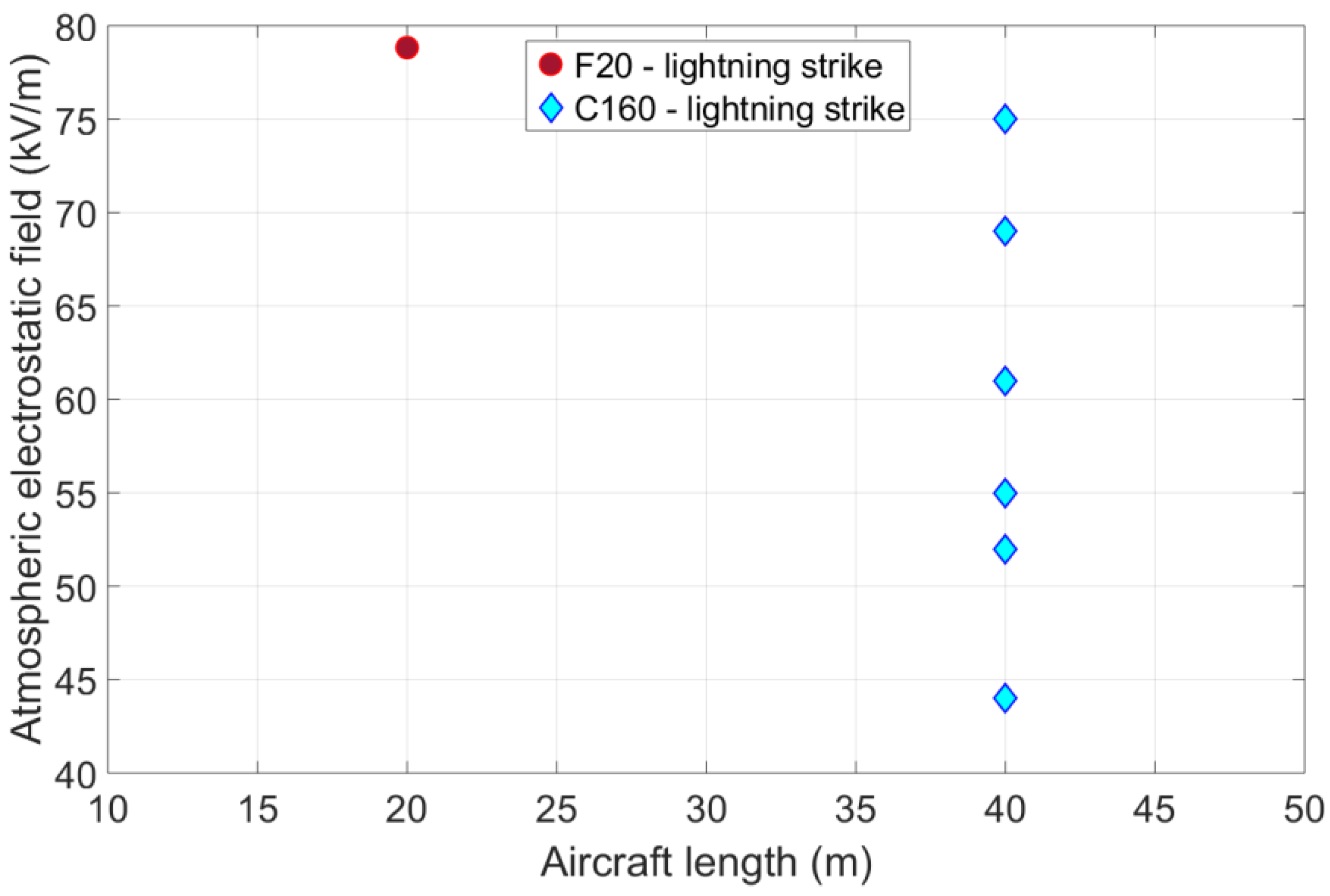
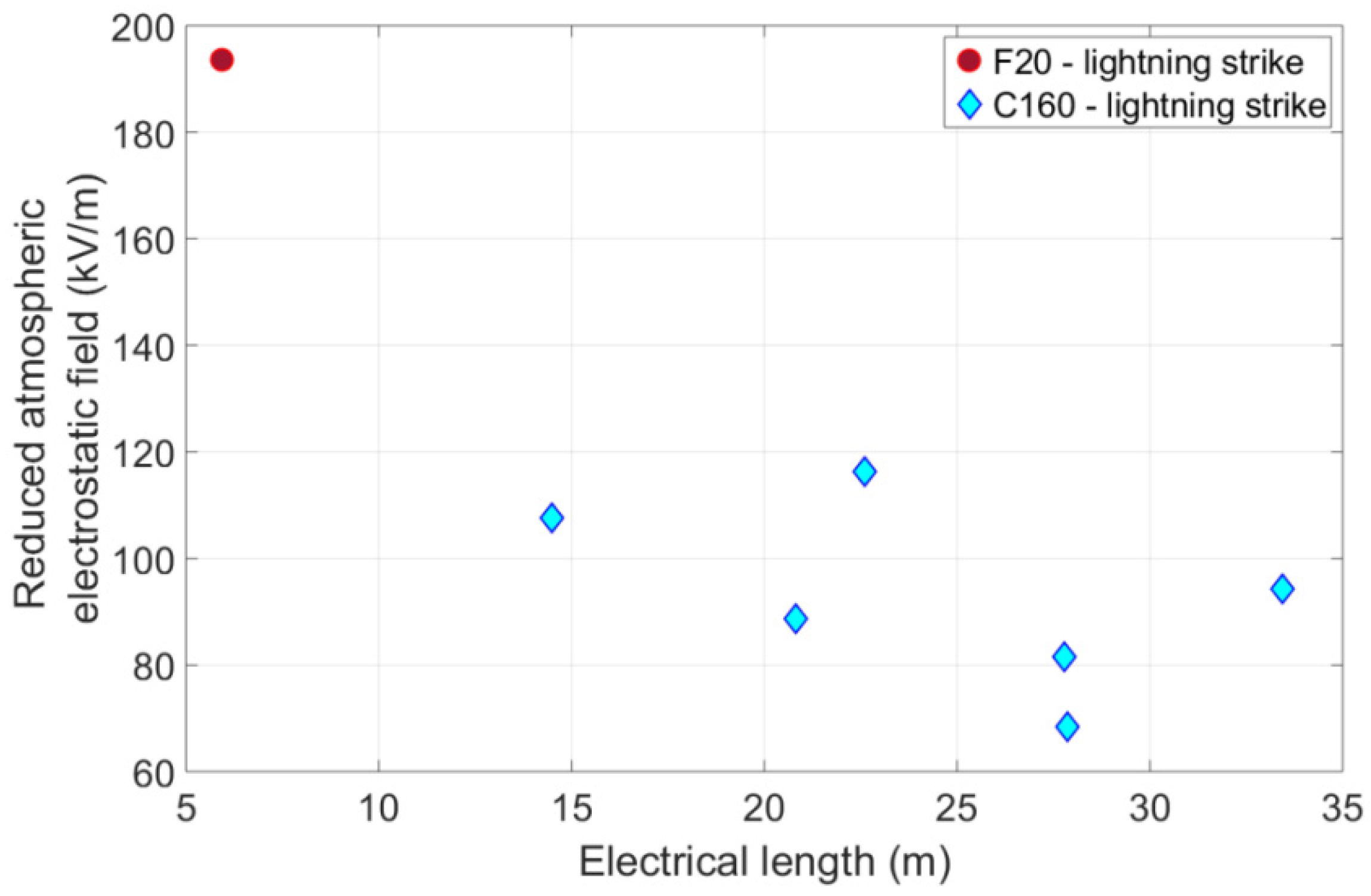
• The electrical length of the aircraft depends on the direction of the atmospheric electric field in regard to the aircraft orientation. If the electric field component is vertical, the length is the height of the aircraft. If the field is along the fuselage, the electrical length is the aircraft length. For a given atmospheric electrostatic field direction, the electrical length H of the aircraft is computed as follows:

  ○

  The geometry of the aircraft is projected on a line generated by the field direction $\overrightarrow{{\mathrm{E}}_0}$ (cf. Figure 14);

  ○

  The electrical length of the aircraft for this electric field direction is the distance H (cf. Figure 14).

Figure 14. Illustration of the computation of electrical length H of the aircraft for a given direction of the atmospheric electrostatic field.

Figure 14. Illustration of the computation of electrical length H of the aircraft for a given direction of the atmospheric electrostatic field.

The result of this processing is shown in Figure 15. The module of the atmospheric electrostatic field brought back to the mean sea level (reduced atmospheric electrostatic field) is plotted as a function of the electrical length of the aircraft. The red circle is associated with the lightning strike to the F20 of the 8 of October 2018 (Figure 12b). The blue diamonds correspond to the lightning strikes of the C160. The figure shows the effect of the electrical length on the lightning-triggered threshold. The longer the aircraft is, the lower the reduced atmospheric electrostatic field to trigger lightning is. It is not easy from this low amount of lightning strike data to define an accurate frontier between no risk and risk of lightning strike of the aircraft. On the C160, we do not observe any lightning strike for a reduced atmospheric electrostatic field lower than 60 kV·m^-1. On the F20, we can go further because we have all the recordings of the field mills.

Figure 16a represents the reduced atmospheric electrostatic field and the associated electrical length for the seven IOP flights of EXAEDRE with a colored differentiation between the flights. The IOP 8 flight presents a few values higher than 150 kV·m⁻¹ for a small electrical length (representing a vertical polarization of the aircraft). For the same flight, some values are ranging between 150 and 170 kV·m⁻¹ for the higher electrical length of the F20 associated mainly to a horizontal polarization. It can be also noted that another flight presents reduced atmospheric electrostatic field values higher than 150 kV·m⁻¹ (also mainly to a horizontal polarization), the IOP 2, a flight during which the aircraft was able to fly in deep convective clouds. This fact is also seen in Figure 16b, where the atmospheric electrostatic field magnitude brought back to the mean sea level is plotted as a function of the altitude (with the differentiation of the flight by color). The highest values (for IOP 8 and IOP 2) were measured between 7.9 and 8.4 km. These two altitudes allowed the aircraft to fly close to the convective cells without being in the convective core. Between 5.5 and 9.5 km, a reduced atmospheric electrostatic field value of 60 kV·m⁻¹ (or higher) is commonly measured (cf. Figure 16a) inside or in the vicinity of different convective clouds during the EXAEDRE campaign without triggering lightning on the F20. On contrary, for the C160, this value can generate a lightning strike to this aircraft (cf. Figure 15).

5. Conclusions

During the EXAEDRE in-flight campaign, ONERA has measured the atmospheric electrostatic field by using the AMPERA system integrated on the Falcon 20 of SAFIRE. This campaign took place in Corsica in September and October 2018. The AMPERA system is composed of a set of eight field mill sensors. Due to the configuration of two sensors, to retrieve the atmospheric electrostatic field, six sensors have been used. The evaluation of the error for this configuration shows that the maximum global error on each atmospheric electrostatic field component ranges between +/−5 and 8%, and there is a maximum global error of 4% for the atmospheric electrostatic field magnitude when the aircraft potential is lower than 10 times the value of the component (or the magnitude of the electrostatic field), which represents 90% of the cases.

Most of the significant values of atmospheric electrostatic field magnitude retrieved during this campaign occur between 5.5 and 9.5 km, which is consistent with past studies that describe the altitude of initiation of lightning flash [34,35]. The highest value of electrostatic field recorded during these flights was around 79 kV·m⁻¹ at 8400 m of altitude, which is equivalent to a reduced atmospheric electrostatic field of 194 kV·m⁻¹.

In order to compare this value to the ones obtained during the C160 in-flight campaign, a method was proposed to take into account the altitude effect and the size of the aircraft. The results show that the longer the aircraft is, the lower the reduced atmospheric electric field to trigger a lightning. From the few measured points (several for the C160, but only a single lightning strike for the F20 during the EXAEDRE campaign), it is not possible to infer a lightning strike threshold for a given aircraft. On contrary, the hours of flight of the F20 show that for a reduced atmospheric electrostatic field lower than 160 kV·m⁻¹, no lightning strike of the aircraft occurred, even if natural lightning flashes occurred in the surrounding of the plane (in an area of a few kilometers to 30 km).

References

1. Delannoy, A.; Gondot, P. Airborne Measurements of the Charge of Precipitating Particles Related to Radar Reflectivity and Temperature within two Different Convective Clouds. AerospaceLab 2012, 5, 1–8. Available online: https://aerospacelab.onera.fr/al5/airborne-measurements-of-the-charge-of-precipitating-particles-related-to-radar-reflectivity-and-temperature-within-two-diff (accessed on 3 November 2021).
2. Laroche, P.; Blanchet, P.; Delannoy, A.; Issac, F. Experimental Studies of Lightning Strikes to Aircraft. AerospaceLab 2012, 5, 1–13. Available online: https://aerospacelab.onera.fr/al5/experimental-studies-of-lightning-strikes-to-aircraft (accessed on 3 November 2021).
3. Rust, W.D.; MacGorman, D.R. Techniques for Measuring Electrical Parameters of Thunderstorms. In Instruments and Techniques for Thunderstorm Observation and Analysis; Kessler, E., Ed.; U. Oklahoma Press: Norman, OK, USA, 1988; pp. 91–118. [Google Scholar]
4. MacGorman, D.R.; Rust, W.D. The Electrical Nature of Storms; Oxford University Press: New York, NY, USA, 1998. [Google Scholar]
5. Kasemir, H.W. The cylindrical field mill. Meteorol. Rundsch. 1972, 25, 33–38. [Google Scholar]
6. Jones, J.J. Electric charge acquired by airplanes penetrating thunderstorms. J. Geophys. Res. Atmos. 1990, 95, 16589–16600. [Google Scholar] [CrossRef]
7. Chauzy, S.; Médale, J.C.; Prieur, S.; Soula, S. Multilevel measurement of the electric field underneath a thundercloud: 1. A new system and the associated data processing. J. Geophys. Res. Atmos. 1991, 96, 22319–22326. [Google Scholar] [CrossRef]
8. Winn, W.P.; Byerley, L.G., III. Electric field growth in thunderclouds. Q. J. R. Meteorol. Soc. 1975, 101, 979–994. [Google Scholar] [CrossRef]
9. Marshall, T.C.; Rust, W.D. Electric field soundings through thunderstorms. J. Geophys. Res. Atmos. 1991, 96, 22297–22306. [Google Scholar] [CrossRef]
10. Stolzenburg, M.; Rust, W.D.; Smull, B.F.; Marshall, T.C. Electrical structure in thunderstorm convective regions: 1. Mesoscale convective systems. J. Geophys. Res. Atmos. 1998, 103, 14059–14078. [Google Scholar] [CrossRef]
11. Gunn, R. Electric Field Intensity Inside of Natural Clouds. J. Appl. Phys. 1948, 19, 481–484. [Google Scholar] [CrossRef]
12. Marshall, T.C.; Rison, W.; Rust, W.D.; Stolzenburg, M.; Willett, J.C.; Winn, W.P. Rocket and balloon observations of electric field in two thunderstorms. J. Geophys. Res. Atmos. 1995, 100, 20815–20828. [Google Scholar] [CrossRef]
13. Laroche, P. Airborne measurements of electrical atmospheric field produced by convective clouds. Rev. Phys. Appliquée 1986, 21, 809–815. [Google Scholar] [CrossRef]
14. Boulay, J.L.; Laroche, P. Aircraft potential variation in flight. Int. Aerosp. Conf. Light. Static Electr. 1982, 1982, 1–19. [Google Scholar]
15. Bouchard, A.; Lalande, P.; Laroche, P.; Blanchet, P.; Buguet, M.; Chazottes, A.; Strapp, J.W. Relationship between airborne electrical and total water content measurements in ice clouds. Atmos. Res. 2020, 237, 104836. [Google Scholar] [CrossRef]
16. Koshak, W.J.; Bailey, J.; Christian, H.J.; Mach, D.M. Aircraft electric field measurements: Calibration and ambient field retrieval. J. Geophys. Res. 1994, 99, 22781–22792. [Google Scholar] [CrossRef]
17. Koshak, W.J. Retrieving Storm Electric Fields from Aircraft Field Mill Data. Part I: Theory. J. Atmos. Ocean. Technol. 2006, 23, 1289–1302. [Google Scholar] [CrossRef]
18. Mach, D.M.; Koshak, W.J. General Matrix Inversion Technique for the Calibration of Electric Field Sensor Arrays on Aircraft Platforms. J. Atmos. Ocean. Technol. 2007, 24, 1576–1587. [Google Scholar] [CrossRef] [Green Version]
19. Winn, W.P. Aircraft measurement of electric field: Self-calibration. J. Geophys. Res. Atmos. 1993, 98, 7351–7365. [Google Scholar] [CrossRef]
20. Bateman, M.G.; Stewart, M.F.; Podgorny, S.J.; Christian, H.J.; Mach, D.M.; Blakeslee, R.J.; Bailey, J.C.; Daskar, D. A Low-Noise, Microprocessor-Controlled, Internally Digitizing Rotating-Vane Electric Field Mill for Airborne Platforms. J. Atmos. Ocean. Technol. 2007, 24, 1245–1255. [Google Scholar] [CrossRef] [Green Version]
21. Mach, D.M. Technique for Reducing the Effects of Nonlinear Terms on Electric Field Measurements of Electric Field Sensor Arrays on Aircraft Platforms. J. Atmos. Ocean. Technol. 2015, 32, 993–1003. [Google Scholar] [CrossRef]
22. Mazur, V.; Ruhnke, L.H.; Rudolph, T. Effect of E-field mill location on accuracy of electric field measurements with instrumented airplane. J. Geophys. Res. Atmos. 1987, 92, 12013–12019. [Google Scholar] [CrossRef]
23. Mach, D.M.; Blakeslee, R.J.; Bateman, M.G.; Bailey, J.C. Electric fields, conductivity, and estimated currents from aircraft overflights of electrified clouds. J. Geophys. Res. Atmos. 2009, 114, 1–15. [Google Scholar] [CrossRef]
24. Baumgardner, D.; Brenguier, J.L.; Bucholtz, A.; Coe, H.; DeMott, P.; Garrett, T.J.; Gayet, J.F.; Hermann, M.; Heymsfield, A.; Korolev, A.; et al. Airborne instruments to measure atmospheric aerosol particles, clouds and radiation: A cook’s tour of mature and emerging technology. Atmos. Res. 2011, 102, 10–29. [Google Scholar] [CrossRef] [Green Version]
25. Lawson, R.P.; O’Connor, D.; Zmarzly, P.; Weaver, K.; Baker, B.; Mo, Q.; Jonsson, H. The 2D-S (Stereo) Probe: Design and Preliminary Tests of a New Airborne, High-Speed, High-Resolution Particle Imaging Probe. J. Atmos. Ocean. Technol. 2006, 23, 1462–1477. [Google Scholar] [CrossRef] [Green Version]
26. Lawson, R.P.; Baker, B.; Pilson, B.; Mo, Q. In Situ Observations of the Microphysical Properties of Wave, Cirrus, and Anvil Clouds. Part II: Cirrus Clouds. J. Atmos. Sci. 2006, 63, 3186–3203. [Google Scholar] [CrossRef] [Green Version]
27. Protat, A.; Bouniol, D.; Delanoë, J.; O’Connor, E.; May, P.T.; Plana-Fattori, A.; Hasson, A.; Görsdorf, U.; Heymsfield, A.J. Assessment of Cloudsat Reflectivity Measurements and Ice Cloud Properties Using Ground-Based and Airborne Cloud Radar Observations. J. Atmos. Ocean. Technol. 2009, 26, 1717–1741. [Google Scholar] [CrossRef] [Green Version]
28. Delanoë, J.; Protat, A.; Jourdan, O.; Pelon, J.; Papazzoni, M.; Dupuy, R.; Gayet, J.F.; Jouan, C. Comparison of Airborne In Situ, Airborne Radar–Lidar, and Spaceborne Radar–Lidar Retrievals of Polar Ice Cloud Properties Sampled during the POLARCAT Campaign. J. Atmos. Ocean. Technol. 2013, 30, 57–73. [Google Scholar] [CrossRef]
29. Dye, J.E.; Bansemer, A. Electrification in Mesoscale Updrafts of Deep Stratiform and Anvil Clouds in Florida. J. Geophys. Res. Atmos. 2019, 124, 1021–1049. [Google Scholar] [CrossRef]
30. Marshall, T.C.; Stolzenburg, M.; Maggio, C.R.; Coleman, L.M.; Krehbiel, P.R.; Hamlin, T.; Thomas, R.J.; Rison, W. Observed electric fields associated with lightning initiation. Geophys. Res. Lett. 2005, 32, 1–5. [Google Scholar] [CrossRef] [Green Version]
31. Stolzenburg, M.; Marshall, T.C. Charge Structure and Dynamics in Thunderstorms. Space Sci. Rev. 2008, 137, 355–372. [Google Scholar] [CrossRef]
32. Lalande, P.; Bondiou-Clergerie, A.; Bacchiega, G.; Gallimberti, I. Observations and modeling of lightning leaders. Comptes Rendus Phys. 2002, 3, 1375–1392. [Google Scholar] [CrossRef]
33. Willett, J.C.; Davis, D.A.; Laroche, P. An experimental study of positive leaders initiating rocket-triggered lightning. Atmos. Res. 1999, 51, 189–219. [Google Scholar] [CrossRef]
34. Coquillat, S.; Defer, E.; De Guibert, P.; Lambert, D.; Pinty, J.P.; Pont, V.; Prieur, S.; Thomas, R.J.; Krehbiel, P.R.; Rison, W. SAETTA: High-resolution 3-D mapping of the total lightning activity in the Mediterranean Basin over Corsica, with a focus on a mesoscale convective system event. Atmos. Meas. Tech. 2019, 12, 5765–5790. [Google Scholar] [CrossRef] [Green Version]
35. Ribaud, J.F.; Bousquet, O.; Coquillat, S. Relationships between total lightning activity, microphysics and kinematics during the 24 September 2012 HyMeX bow-echo system. Q. J. R. Meteorol. Soc. 2016, 142, 298–309. [Google Scholar] [CrossRef] [Green Version]
Figure 1. Electric field mill used during the EXAEDRE campaign. (a) General view of the sensor; (b) Sensor implemented on a dummy window.
Atmosphere 12 01645 g001
Figure 2. Photography of the Falcon 20 (F20) of SAFIRE (https://www.safire.fr/en/, accessed on 2 December 2021) on which the location of the eight field mills is shown.
Atmosphere 12 01645 g002
Figure 3. Three-dimensional shape model of the Falcon 20 aircraft, including the pods. The reference presented here is the aircraft reference: the x-axis is from the nose to the tail, the y-axis is from the left wing to the right wing, and the z-axis is upward).
Atmosphere 12 01645 g003
Figure 4. (a) Electric field on the electric field mills on the F20 the 13th of September 2018 (IOP 1, i.e., first Intensive Observation Period). (b) Schematic orientation of electric field on the aircraft surface when the electric potential Va of the aircraft is negative in this example. There is no atmospheric electric field.
Atmosphere 12 01645 g004
Figure 5. (a) Electric field on the electric field mills on the F20 the 20th of September 2018 (IOP 4). (b) Schematic orientation of electric field on the aircraft surface when the aircraft flies inside an atmospheric electrostatic field E o . The thick dashed line illustrates the position of charge separation when the aircraft is polarized by this direction of atmospheric electrostatic field in regard to the aircraft. The thin dashed lines represent the electric field lines.
Atmosphere 12 01645 g005
Figure 6. Cumulative distribution of the ratio of the aircraft potential on the magnitude of the atmospheric electrostatic field for the wall flight of the EXAEDRE campaign when an atmospheric electrostatic field magnitude higher than or equal to 6 kV/m is measured (the abscissa axis is the class of this ratio, the ordinate axis represents the normalized occurrence of the values of the ratio).
Atmosphere 12 01645 g006
Figure 7. Trajectories of the seven IOP (Intense Observation Period) flights kept for the analysis.
Atmosphere 12 01645 g007
Figure 8. Flight IOP 4 between 07:26 and 07:35 UTC: illustration of the cloudy area in which the electric field has been measured, which is followed by an area with aircraft potential, before leaving the cloud. During the pass in the cloud area, the aircraft flies at an altitude of 7300 m (+/−20 m). (a) Temporal evolution of measurements of the six field mills. (b) In the same period, atmospheric electrostatic field magnitude, its components (left axis), and the aircraft potential (right axis) retrieved from the six field mills.
Atmosphere 12 01645 g008
Figure 9. Flight IOP 8–between 09:20:30 and 09:26 UTC and 10:20 and 10:23 UTC: (a,b): Illustration of polarization of the aircraft measured by the field mills. (c,d): For the same periods, temporal evolution of magnitude of the atmospheric electrostatic field, its components (left axis), and aircraft potential (right axis) retrieved by the six field mills measurements. During the both passes, the aircraft flies at an altitude of 7500 m (+/−20 m).
Atmosphere 12 01645 g009
Figure 10. For atmospheric electrostatic field magnitude ≥10 kV/m: magnitude of the atmospheric electrostatic field plotted as a function of the altitude. The color represents the number of the flights.
Atmosphere 12 01645 g010
Figure 11. (a) Time evolution of the electric field measured by each field mill on the 8 of October 2018 (IOP 8). The time is UTC. The black arrows show periods where the aircraft was outside the clouds. The altitude of the aircraft was about 7500 m before 10:24 UTC and about 8400 m after this time and before the next phase of cloud exploration at 10:28 UTC. (b) Electric fields measured by the six field mills on the fuselage around the lightning strike time. During this pass, the altitude of the aircraft was about 8400 m.
Atmosphere 12 01645 g011
Figure 12. (a) Temporal evolution of the atmospheric electrostatic field components (Ex, Ey, Ez) in the aircraft reference and the aircraft potential of the aircraft on the 8 of October 2018 (IOP 8) during the same period as in Figure 11a. (b) Temporal evolution of the atmospheric electrostatic field magnitude. The red filled circle is associated with the electrostatic field when the lightning strikes the F20.
Atmosphere 12 01645 g012
Figure 13. Comparison between the atmospheric electrostatic fields during a lightning strike to the aircraft for the F20 and C160 as a function of the length of the aircraft.
Atmosphere 12 01645 g013
Figure 15. Comparison between reduced atmospheric electrostatic field values for the F20 and C160 as a function of the electrical length of the aircraft (H).
Atmosphere 12 01645 g015
Figure 16. In both cases, the color represents the number of the flight. (a) For the F20 data, there is a reduced atmospheric electrostatic field as a function of the electrical length with a differentiation of the flights by the color dots. The biggest point is associated with the value of the aircraft lightning strike of the F20 during the IOP 8. (b) The same figure as Figure 10 but with the reduced atmospheric electrostatic field.
Atmosphere 12 01645 g016