1. Introduction
The problem of the atmospheric environment has received widespread public attention. The quality of the air has a greater impact on human health and the ecological environment. An increasingly serious air pollution issue has played a role in every corner of affecting people’s daily lives. The air quality index (AQI) is an index system that quantitatively describes the air quality status. The higher the value and level, the more serious the air quality and pollution. It mainly includes fine particulate matter (PM
2.5), inhalable particulate (PM
10), sulfur dioxide (SO
2), nitrogen dioxide (NO
2), ozone (O
3), and carbon monoxide (CO). According to different limits of pollutants, it is converted into an air quality index according to different target concentrations. With urbanization and industrialization developments, air pollution in many cities hides an alarming reality throughout China. In 2019, WHO announced the top ten threats to global public health, of which air pollution is considered the biggest threat [
1]. In 2016, the number of premature deaths caused by PM
2.5 in the world was about 4.2 million [
2]. Haze is one of the most serious environmental problems in China, the Chinese government plans to implement strict control measures to reduce the PM
2.5 concentration [
3]. CO can indirectly aggravate the greenhouse effect and participate in the formation of near-surface photochemical smog, which is an important pollution component to measure the regional atmospheric environment [
4]. A high concentration of O
3 will affect the human respiratory tract, cardiovascular and immune system, leading to asthma, respiratory tract infection, stroke, and arrhythmia [
5,
6,
7]. PM10, with a long retention time in the atmosphere and a relatively large specific surface area, is easy to carry with a large number of toxic and harmful substances. PM
10 can enter human alveoli through the respiratory tract and even participate in blood circulation, which will cause more obvious harm to human body [
8]. When NO
2 enters the alveoli, it causes bronchitis, pneumonia, emphysema, and SO2 with high concentration [
9]. It is estimated that the number of deaths caused by indoor and outdoor air pollution in China is 2.5 million people per year [
10]. The reasonable assessment and control of air quality can help reduce the adverse effects of air pollution. Therefore, it is necessary to accurately predict the concentration of air pollutants to help management departments and potentially hazardous groups in various regions to reduce the impact of air pollutants.
In recent years, machine learning and deep learning models have been gradually applied to predict the concentration of air pollutants. Feng et al. [
11] used artificial neural networks and wavelet transform to predict PM
2.5 concentrations based on geographic models. Ke et al. proposed a stack selection ensemble algorithm for PM
2.5 prediction [
12], Zhou et al. exerted the seasonal gray model to predict the air quality indicators in the Yangtze River Delta of China [
13]. Zhang et al. applied the gray multivariate convolution model to predict the daily PM
2.5 and PM
10 concentrations in Shijiazhuang City [
14]. Nouri et al. wielded principal component analysis and artificial neural network (ANN) to predict PM
2.5 concentration in Urmia, Iran [
15]. Zhou et al. fused the multivariate correlation function to the Bayesian model averaging method (CBMA) combined with ANN for PM
2.5 prediction [
16]. Du et al. utilized the multi-objective Harris Hawk optimization (MOHO) algorithm to predict the PM
2.5 and PM
10 hour concentrations in Jinan, Nanjing, Chongqing [
17]. Li et al. made use of integrated reinforcement learning to predict the daily concentration of PM
2.5 [
18]. Guo et al. used Lagrangian and Bayesian methods to predict the hourly concentrations of PM
10 and PM
2.5 in Xingtai [
19].
Aiming at air quality prediction, the main models used in the existing research include the linear regression model [
20] and the generalized weighted mixed model [
21]. With the development of computer technology, machine learning (including deep learning) methods are increasingly used in concentration estimations due to their strong nonlinear modeling ability, such as k-nearest neighbor (KNN) [
22], random forest (RF) [
23], long-term memory network (LSTM) [
24], and convolution neural network (CNN) [
25]. These models all show better performance than traditional statistical models in predicting PM
2.5 concentration and have stronger nonlinear expression capabilities.
Many scholars have begun to try to use deep learning models for prediction. Guo et al. used deep learning methods such as recurrent neural network (RNN) and LSTM to predict PM
2.5 hourly concentration [
26]. Sahin et al. predicted daily PM
2.5 and SO
2 concentrations in Istanbul using convolutional neural network (CNN) [
27]. Sayeed et al. established a prediction model of ozone concentration 24 h in advance using a CNN [
28]. WANG et al. combined a chi-square test (CT) and LSTM network model to predict AQI levels in Shijiazhuang, Hebei Province [
29]. Liu et al. used industrial data to establish a factory aware attentional LSTM neural network (FAALSTM) model to predict PM
2.5 [
30]. Pak et al. used the CNN and LSTM models to predict the daily average concentration of PM
2.5 in Beijing on the second day [
31]. Wen et al. established a spatio-temporal convolutional short-term memory neural network expansion model (C-LSTME) to predict the PM
2.5 hourly concentration in Beijing and China [
32].
The above research verifies the effectiveness of deep learning methods such as CNN and LSTM in the prediction of atmospheric pollutants, and also shows that combined prediction is beginning to be favored by many scholars. Many scholars have begun to pay attention to the influence of other factors on the prediction of atmospheric pollutant concentration. Nourani et al. used temperature, wind speed, humidity, pollutant concentration and other factors as input variables, and used ANN and adaptive neuro-fuzzy inference system (ANFIS) combined with the prediction of CO pollutant concentration [
33]. Heydari et al. proposed a hybrid intelligent model based on LSTM and multiple optimization algorithm (MVO) to predict NO
2 and SO
2 in air pollutants [
34]. Chen et al. predicted PM
2.5 concentration in Zhejiang Province and found that meteorological factors such as temperature, air pressure, evaporation, and humidity have a significant correlation with PM
2.5 concentration [
35]. Zhang et al. found that O
3 hourly mass concentration is related to temperature and sun. There is a positive correlation among radiation, visibility, and wind speed, and a negative correlation with relative humidity and atmospheric pressure. The concentration of NO
2 is positively correlated with relative humidity and atmospheric pressure [
36], Precipitation [
37], season [
38], precipitation [
39], sunshine time [
40], road transportation [
41] and other factors have a significant impact on the concentration of air pollutants. Through the above research, it is found that meteorological factors have a significant impact on the concentration of air pollutants.
In summary, through combing the existing literature, it is found that the research has the following shortcomings: (1) most of the above research focuses on the prediction of a single or two atmospheric pollutants such as PM
2.5 and PM
10, and such models were yet to find the relationship between multiple factors and atmospheric pollutants, so that the predictive performance of atmospheric pollutants cannot be fully utilized; (2) it is difficult for a single LSTM network to mine the relationship and characteristic information among the data; (3) the existing air pollutant concentration prediction models mostly start from a single or two pollutant concentrations to establish corresponding air pollutant concentration prediction models; (4) in the prediction of atmospheric pollutant data, most of the prediction objects are hourly concentration and daily concentration, but the current model fails to consider both predictions, and the prediction accuracy of some prediction models needs to be improved; (5) the existing research on air pollutant concentration prediction still has certain limitations. Most studies only select some important variables in the pollutant concentration data set, and then model the time information to predict the pollutant concentration. There is a lack of deep learning models for predicting the concentration of air pollutants using time information and multivariate time series data in the prediction of pollutant concentration. Therefore, an appropriate algorithm is necessary to be selected to model the irregular temporal information of concentration data and the spatial information of all variables [
42,
43].
The main contributions of this article are as follows:
(1) To establish an air pollutant prediction model that considers the temporal and spatial characteristics of pollutants and the combination of multiple factors. By combining the advantages of the two algorithms of ODMSCNN and LSTM, ODMSCNN has a strong ability to automatically extract features, and LSTM has a strong ability to deal with time series problems. ODMSCNN-LSTM-based air pollutant concentration prediction model is proposed;
(2) PM2.5, PM10, NO2, SO2, O3, CO concentration data are selected as the characteristics of atmospheric pollutants to predict. The temperature (TEM), evaporation (EVP), minimum relative humidity (MI-RHU), maximum wind speed (MM-WIN), precipitation (PRE), sunshine duration (SSD), average wind speed (AV-WIN), and other factors are used as meteorological features;
(3) Perform daily concentration prediction and hourly concentration prediction and compare the performance of each model based on grammar correction MLP, CNN, LSTM, and ODMSCNN-LSTM models;
(4) The proposed model is compared from the perspective of grouped data and multivariate factors, and the performance of ODMSCNN-LSTM in different grouped data sets. The influence of atmospheric pollutant factors and meteorological factors on the prediction of atmospheric pollutant concentration are analyzed.
3. Method
3.1. One-Dimensional Multi-Scale Convolutional Neural Network (ODMSCNN)
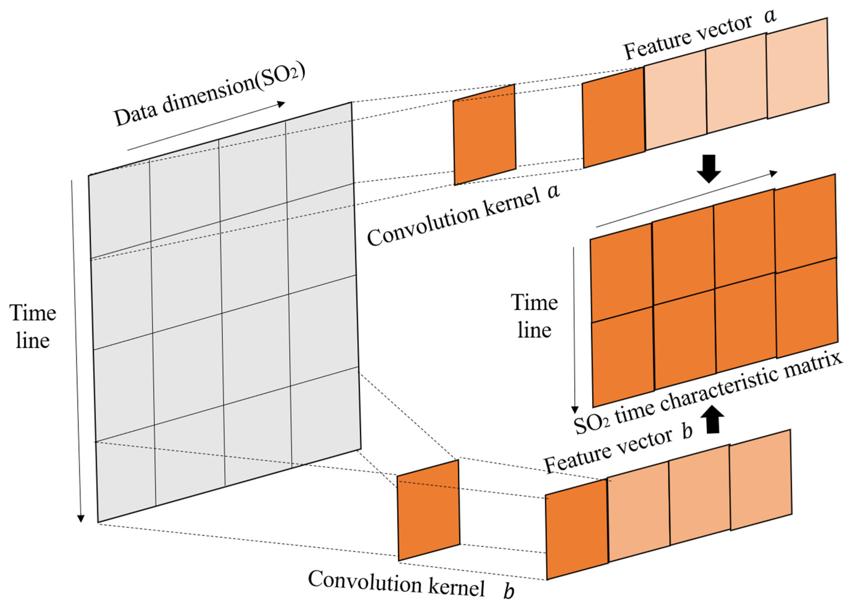
The convolutional neural network is successfully applied to the direction of image recognition, verifying that the network has a powerful effect on the feature extraction ability of feature maps, and this article needs to extract the spatial and temporal features of atmospheric pollutant concentration data and meteorological factors. This paper analyzes the data set and finds that the characteristics of the data are multi-features, which are expressed in the form of numerical values instead of feature maps. Therefore, this paper first preprocesses the data, merges the features of the data into a feature map, and finally inputs them into the convolution neural network to extract the spatial and temporal features.
Taking single-factor SO
2 as an example, the spatio-temporal feature extraction of SO
2 is shown in
Figure 3. The feature map is traversed from left to right on the data feature axis through a one-dimensional multi-scale convolution kernel (1 × 3, 1 × 5, 1 × 7) to complete the convolution operation; the number of steps is 1, with different convolution kernels. The output feature vectors are spliced and fused, and a single-factor spatial feature relationship is obtained for this purpose. On the time axis, as the convolution kernel traverses from top to bottom to complete the convolution operation, the number of steps is 1, and the local trend of single factor changes over time can be obtained. Finally, the spliced and fused feature vectors are merged in the data feature direction, and the spatio-temporal features of the multi-site SO
2 are output.
The following is the formula derivation of ODMSCNN’s convolution operation on the special whole. The feature map contains
sample data and
air pollutant factors. Then the feature map formula of single factor
i is as follows:
In the formula, is the vector of the single factor at time , represents the group vector of in the time zone [,], and represents the matrix transpose.
The convolution operation multiplies the weight matrix and
(1) Single-factor spatial feature relationship: multiply by on the data feature axis;
(2) Single factor time change feature: multiply by on the time feature axis.
When the first convolution kernel traverses the entire feature map on the time axis, and the number of steps is 1, the feature vector
is obtained, the size of which is
, and the feature vector obtained by multiple convolution kernels
is merged with the size of
in the data feature direction
,
represents the single-factor spatio-temporal characteristic matrix.
So far, the single-factor spatio-temporal feature extraction is completed, but the data set also contains other features, such as NO
2, O
3, CO, etc. Our process includes
factors, so we can extract the
factors through the same operation as above, and then they can be extracted. Single-feature spatio-temporal feature matrix, and then linear splicing and fusion of them, and finally forming a multi-factor fusion spatio-temporal feature matrix
, as shown in Equation (8):
Based on the ODMSCNN convolution neural network, the space-time characteristics of air quality data are extracted. This method makes a simple transformation of the two-dimensional feature map to form a side-by-side one-dimensional feature map, which makes the network training show better generalization ability. The method of automatic feature extraction by convolutional neural network replaces the traditional manual feature selection method, which makes feature extraction have a more comprehensive and deeper effect.
3.2. Long- and Short-Term Memory Neural Network
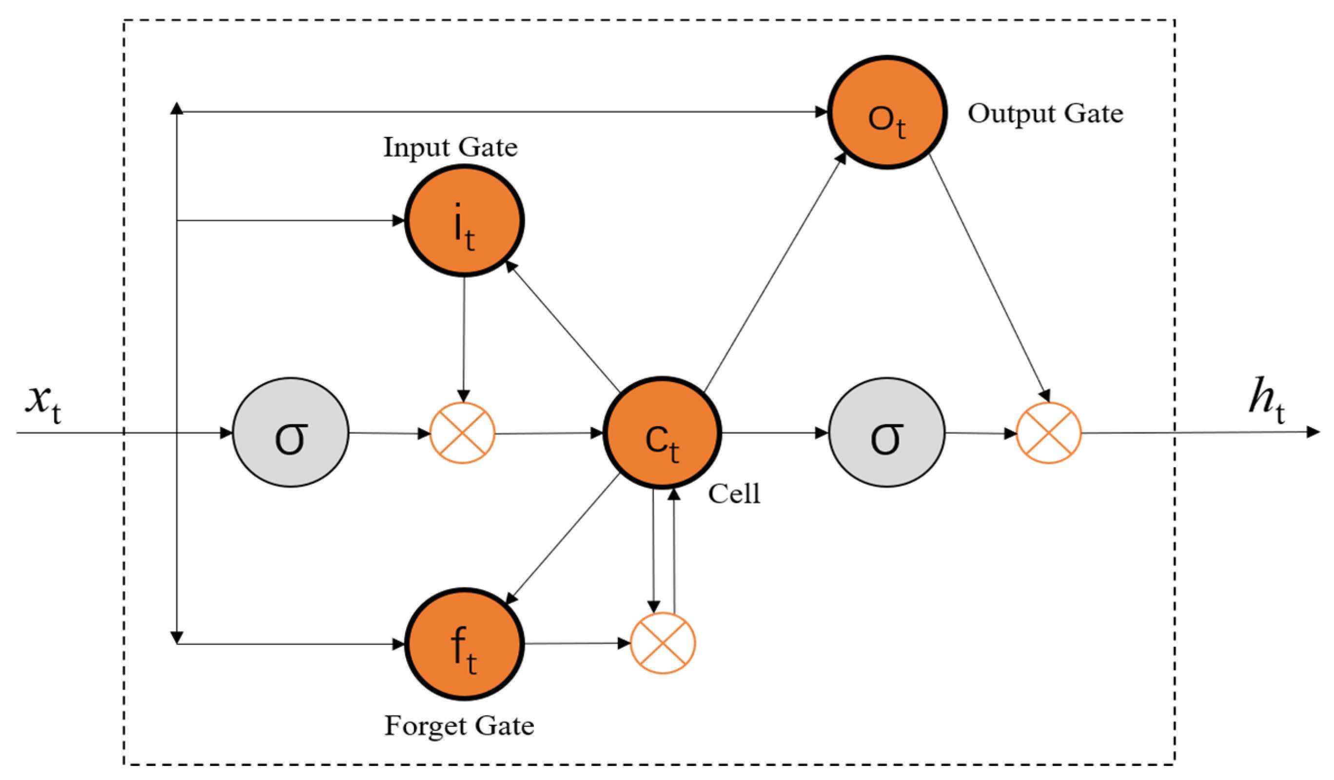
LSTM is an improvement on the RNN. There is a long-term dependence on the problem of RNN’s disappearance and the explosion of gradients during training. LSTM can effectively solve this problem, it introduces a gate mechanism, which makes LSTM have a longer-term memory than RNN and can learn more effectively. In LSTM, each neuron is equivalent to a memory cell (cell, ct). LSTM controls the state of the memory cell through a “gate” mechanism, increasing or deleting the information in it. The structure of LSTM is shown in
Figure 4.
In the LSTM cell structure, the Input Gate () is used to determine what information is added to the cell, and the Forget Gate () is used to determine what information is deleted from the cell. The output gate () is used to determine what information is output from the cell. The complete training process of LSTM is that at each time , the three gates receive the input vector at time and the hidden state of the LSTM at time and the information of the memory unit , and then perform the received information Logical operation, the logical activation function decides whether to activate it, and then synthesize the processing result of the input gate and the processing result of the forgetting gate to generate a new memory unit , and finally obtain the final output result through the nonlinear operation of the output gate. The calculation formula for each process is as follows.
Input gate calculation formula:
Forget Gate calculation formula:
Output Gate calculation formula:
Memory unit calculation formula, Hidden state:
Hidden state calculation formula:
Among them, σ is generally a nonlinear activation function, such as a sigmoid or tanh function. , , , are the weight matrices of nodes connected to the input vector for each layer, , , , are the weight matrices connected to the previous short-term state ht-1 for each layer, , , , are the offset terms of each layer node.
In short, the input gate in LSTM can identify important inputs, and the forget gate can reasonably retain important information and extract it when needed. Therefore, this feature of LSTM can effectively identify long-term patterns such as time series, making training convergence faster.
3.3. ODMSCNN-LSTM-Based Atmospheric Pollutant Concentration Prediction Model
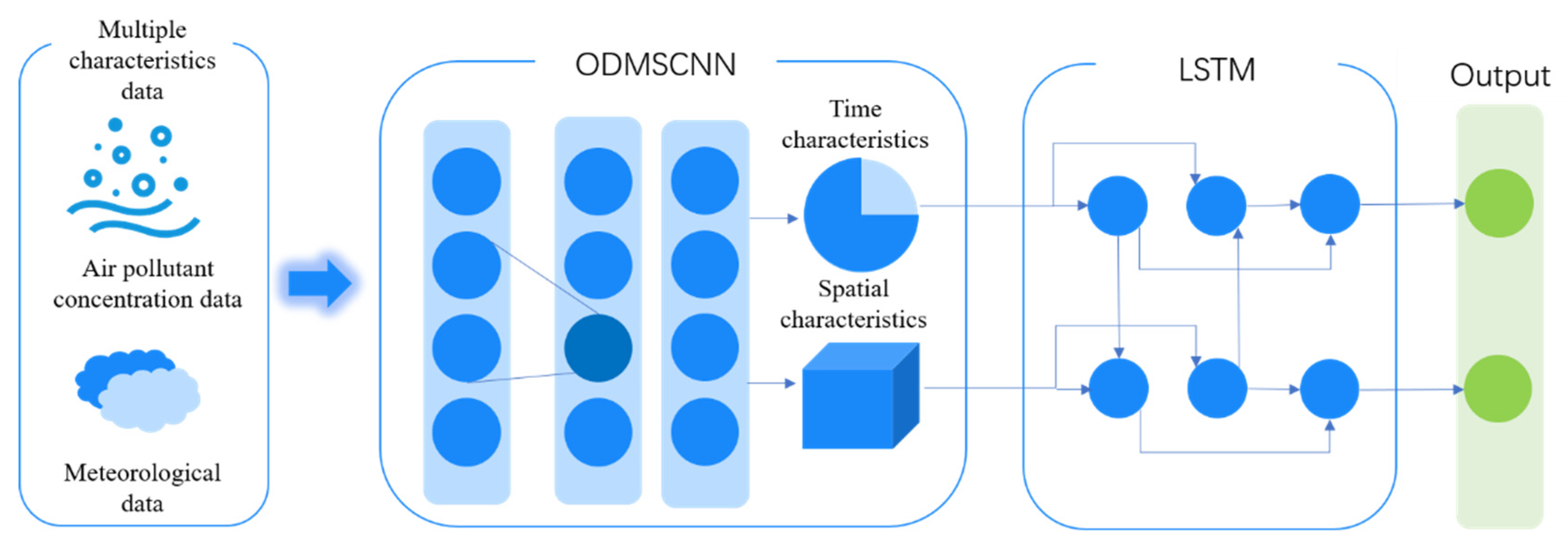
As shown in
Figure 5, the model is composed of two parts: ODMSCNN and LSTM. The temporal and spatial features of multiple variable data are extracted through ODMSCNN, and then pass to the LSTM layer. The LSTM layer models the spatio-temporal feature information input by the ODMSCNN layer, and then ODMSCNN and LSTM pass through the connection layer and predict the concentration of air pollutants.
First of all, the starting layer of the model is composed of ODMSCNN to accept multiple variable inputs of atmospheric pollutant accumulation data, such as relevant atmospheric pollutant factors and meteorological factors. The factor variables are input into the convolutional neural network, and the spatio-temporal feature relationship among each of them is extracted through ODMSCNN. There are multiple hidden layers involved in the feature extraction process of ODMSCNN. The deeper the number of layers, the deeper the network depth. The extracted features are used as the input of the LSTM layer. Secondly, the hidden layer content of CNN consists of a convolutional layer, an activation function and a pooling layer. The convolution operation simulates the response of a single neuron to visual stimulation, that is, when processing the time series, each neuron processes the received data and extracts the data features. The convolution operation can reduce the number of parameters and make the CNN-LSTM network deeper. Finally, dimensionality reduction and feature extraction are performed on the data through the CNN convolutional layer, and the single-factor spatio-temporal feature relationship extracted by ODMSCNN is simply linearly spliced and fused to obtain the mutual spatio-temporal feature relationship of multiple factors. Avoid over-fitting phenomenon, improve the robustness in the feature extraction process, and apply LSTM to solve the problem of long-term data memory, and realize the source data fusion perception and multi-layer perception.
3.4. Prediction Process of Atmospheric Pollutant Concentration
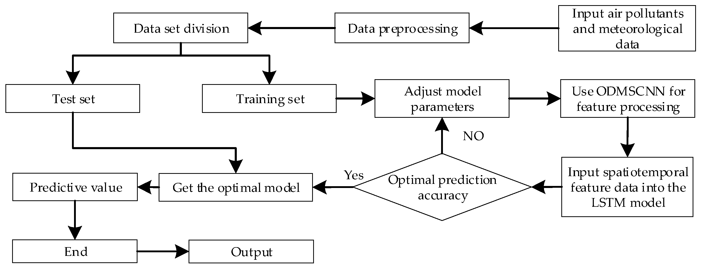
Figure 6 is the forecasting process of atmospheric pollutant concentration, including five parts of data pre-processing, extract features, nodal features, model test and data prediction.
(1) Data processing preparation. Data preprocessing is performed in the original data of atmospheric pollutant concentration prediction, and the data set is divided into training set, verification set, and test set. The training set is mainly used to train the model. The validation set is used to adjust the parameters of the concentration prediction model, determine the network structure of ODMSCNN and LSTM, and select the number of hidden units. The test set is used to verify the performance of the model;
(2) Feature extract. Input the training set into ODMSCNN to extract spatio-temporal features and input the extracted spatio-temporal features into LSTM for training to find the optimal structure and parameters of the model;
(3) Model tuning. Use training set for model tuning. The experiment process adopts the control variable method. Firstly, determine the initial number of layers and parameters of the ODMSCNN-LSTM model, fix the structure of LSTM, and the number of layers and parameters of ODMSCNN. Secondly, after the best structure of ODMSCNN is determined, adjust the number of layers and parameters of LSTM. Finally, choose the best structure of ODMSCNN-LSTM, and judge whether loss has converged (loss = mae). If it has converged, move to the next step. However, if it has not converged, continue with the previous step until the optimal structure and parameters of the model are found;
(4) Model test. Put the validation set into the trained model for prediction. The evaluation index is used to evaluate the prediction result to determine whether the prediction effect is the best, that is, whether the predicted value achieved the best fitting effect with true value. If the fitting result is the best, the prediction is completed. However, if the fitting effect is not good, go back to the second step to continue iterating the model parameters, and verify the performance and accuracy of the method, analyze and compare the experimental results;
(5) Data prediction. Use the test set data to make predictions. The predicted value is compared with the true value to determine whether the optimal value is obtained. When the optimum is reached, the predicted value is output.
3.5. Model Evaluation Indicators
Root mean square error (RMSE), mean absolute error (MAE), mean absolute percentage error (MAPE), and goodness of fit are two commonly used cross-validation indicators. This study uses these four indicators to evaluate the model.
The specific formula derivation of the LSTM is as follows:
where
is the predicted values of air pollutants,
is the true values of air pollutants, and
is the number of test samples. Generally, the larger the value of RMSE and MAE, the greater the error and the lower the prediction accuracy of the model. MAPE is the most intuitive criterion for prediction accuracy. When MAPE tends to 0%, it means the model is perfect. When MAPE tends to 100%, it means that the model is inferior. Generally, it can be considered that the prediction accuracy is higher when the MAPE is less than 10% [
49].
4. Results
4.1. Daily Concentration Data Prediction
The daily concentration data from January 2014 to December 2020 is selected.
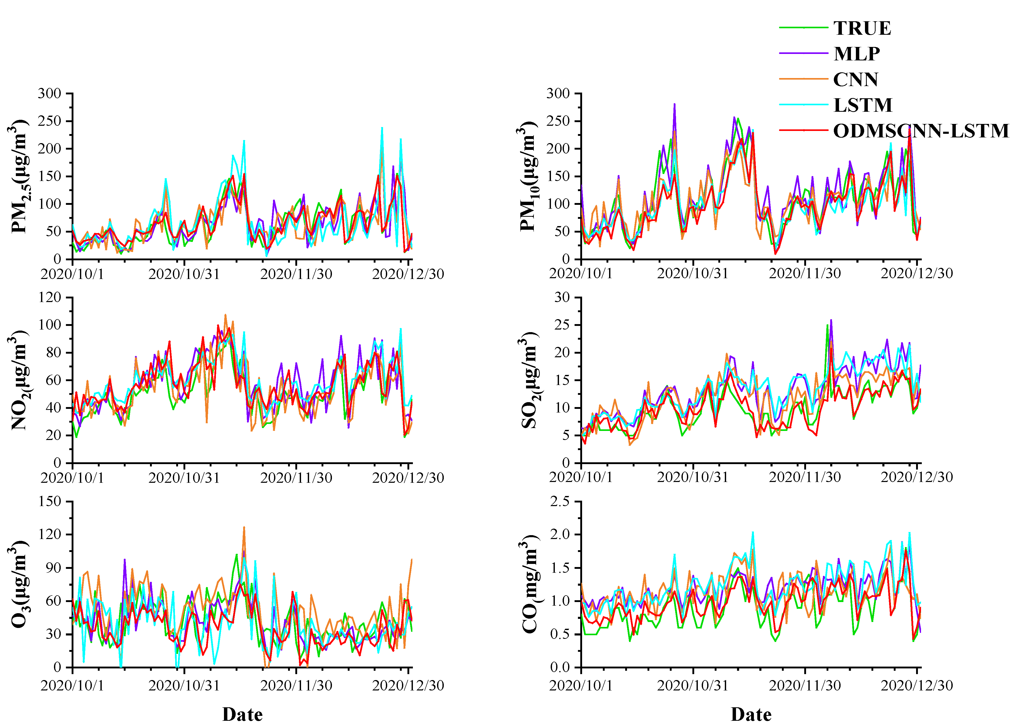
Table 2 shows the daily air pollutant concentration prediction results of different models. In terms of prediction, the order of RMSE is arranged in descending order of MLP, CNN, LSTM, and ODMSCNN-LSTM.
As shown in
Figure 7, the four prediction models are used to predict the concentrations of six kinds of air pollutants, respectively. The forecast results of the six air pollutant concentrations in four different models are drawn. The green and red lines of the prediction results represent the actual and ODMSCNN-LSTM predicted air pollutant concentrations, respectively. By comparing the predicted values of the four models with their corresponding true values, it is found that the predicted value of ODMSCNN-LSTM shows its more accurate prediction performance compared with the other three models. It can be seen from the six air pollutant concentration prediction curves that the constructed ODMSCNN-LSTM prediction model well reflects the timeliness and nonlinearity of the air pollutant concentration distribution. This model responds quickly both to short-term and long-term predictions, and it performs well even when the six kinds of air pollutant concentration suddenly change. Due to the great change of air pollutant concentration between 2014 and 2020, the RMSE value and the maximum average error value of the ODMSCNN-LSTM model for daily concentration prediction of air pollutants are greater than those of the subsequent hourly data, but the prediction effect of the ODMSCNN-LSTM model is better than other prediction models.
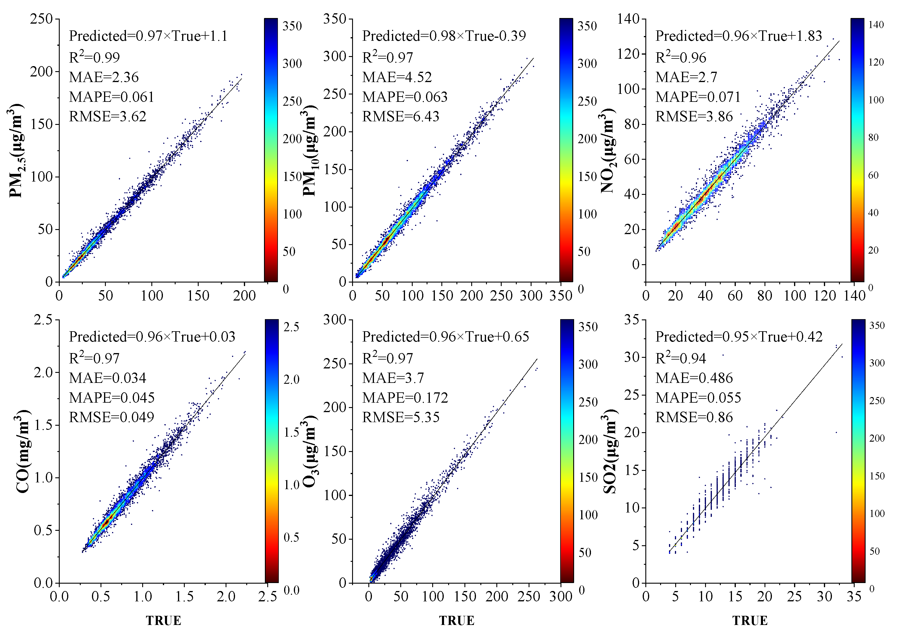
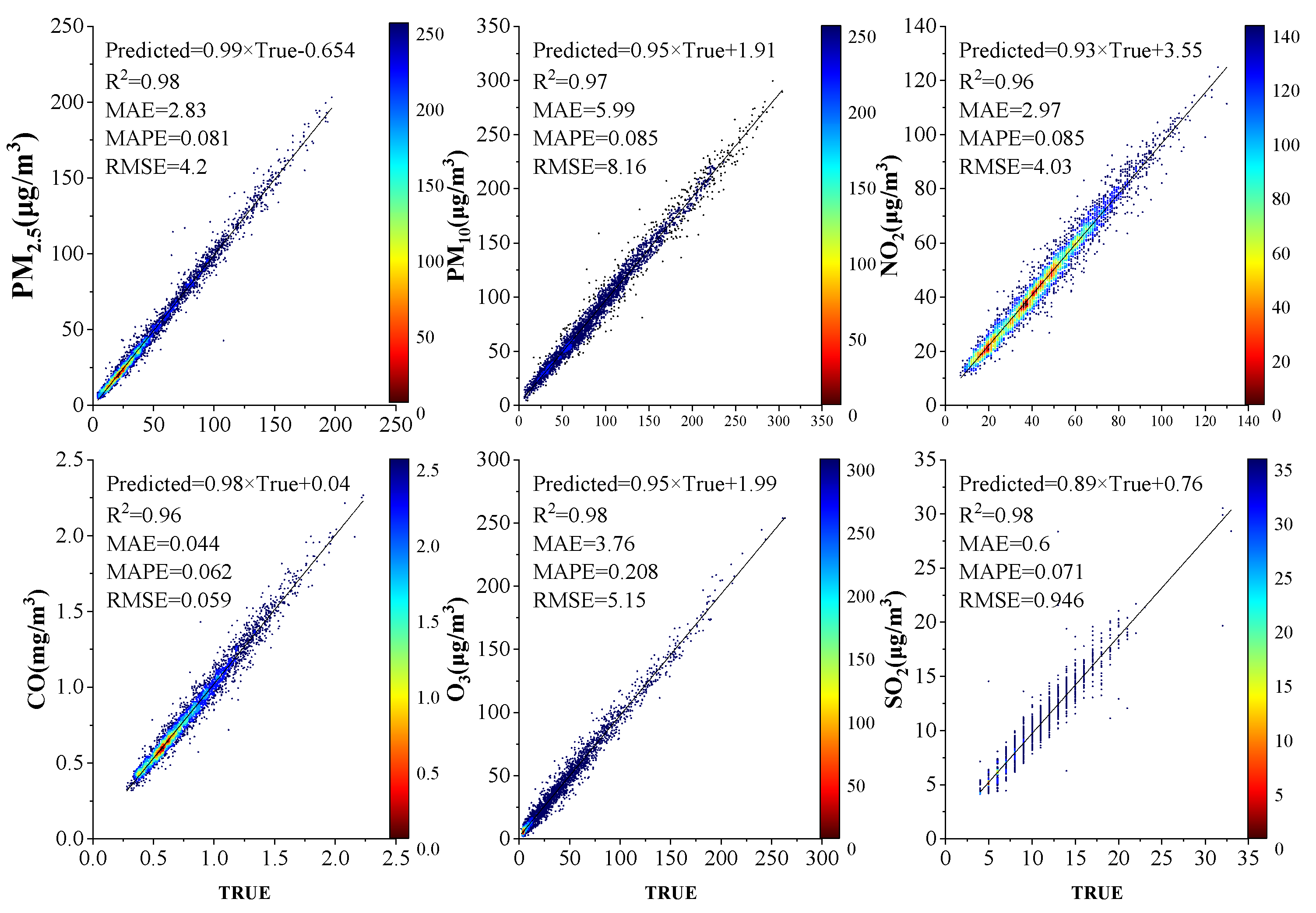
4.2. Hourly Concentration Data Prediction
In order to better verify the validity and prediction ability of the model, the hourly concentration data from 1 January 2019 to 31 December 2020 were selected in this paper. The data from the test set were used as a new prediction range and the performance of the air pollutant prediction model was evaluated again.
According to the data in
Table 3, in terms of model performance, the average values of RMSE, MAE, and MAPE, evaluation indexes of six kinds of air pollutants in four prediction models, are arranged in the order of CNN, MLP, LSTM, MSCNN-LSTM. Then, the three evaluation indexes RMSE, MAE, and MAPE of the four models for hourly data are compared. It is found that the all the three indexes provided by the MSMSCNN-LSTM model for all the six air pollutants including PM
2.5 are the lowest.
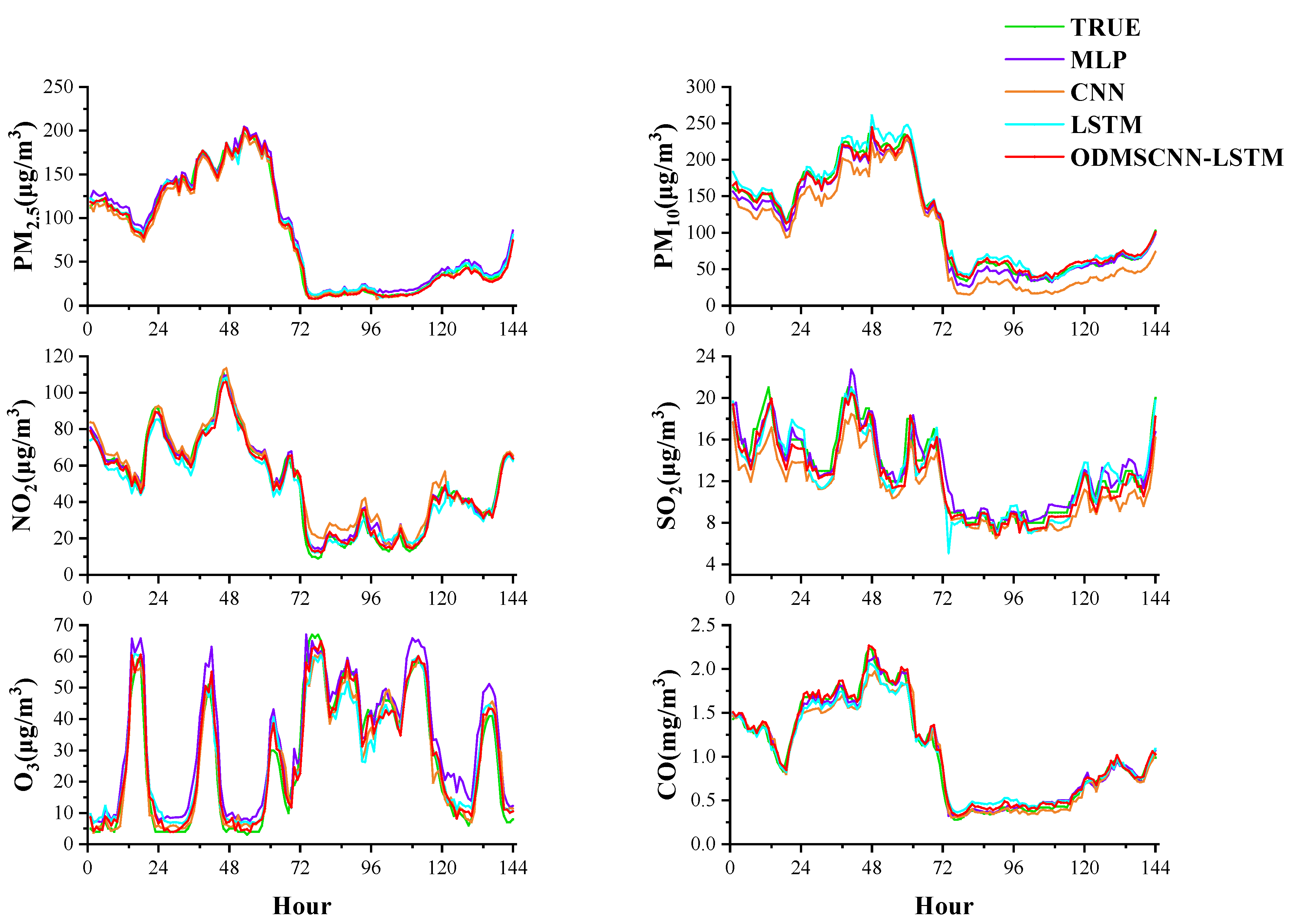
As shown in
Figure 8, the four prediction models are used to predict the concentration of six air pollutants, and their respective prediction results are plotted. The figure shows the concentration prediction results of the six air pollutants for 6 days (144 h in total). The green and red lines represent the actual and ODMSCNN-LSTM predicted air pollutant concentrations, respectively. It can be observed that the ODMSCNN-LSTM model performs best among the four models. Through the comparison of the prediction results of the four models in
Figure 8 the hourly concentration prediction model based on ODMSCNN-LSTM well predicts the 6-day air pollutant concentration distribution and shows good performance. Comparing the hourly concentration data with the daily concentration data. The MSCNN-LSTM model shows a better prediction effect because the average values of its three indexes RMSE, MAE and MAPE for the six air pollutants have increased by 68.87%, 66.36%, and 63.09%, respectively. The reason is that the daily concentration data has fewer samples than hourly data, and the daily concentration data fluctuates greatly, and ODMSCNN-LSTM performs better for large samples of continuous time series data.
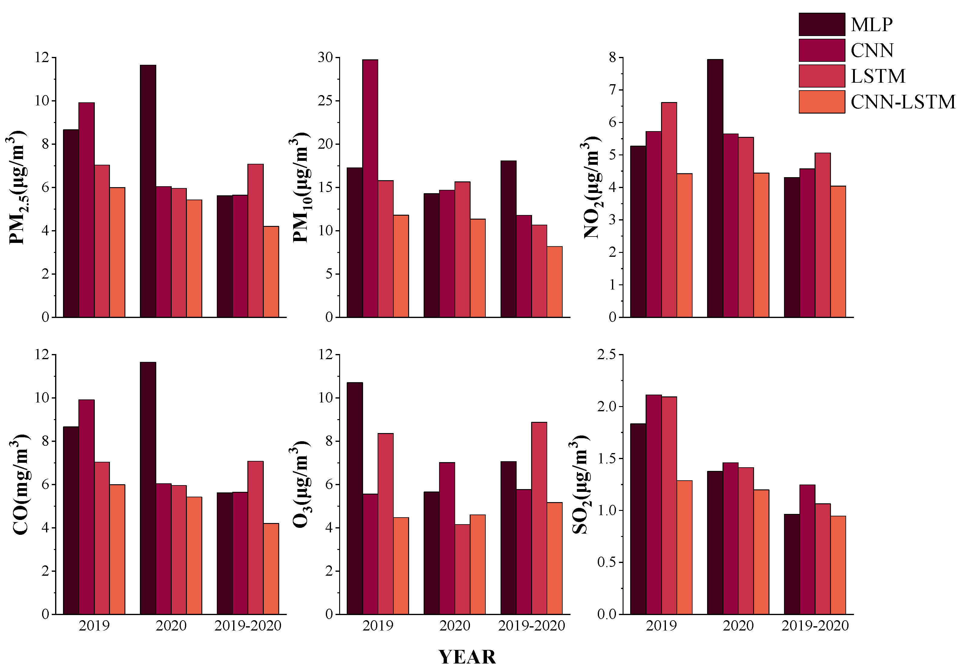
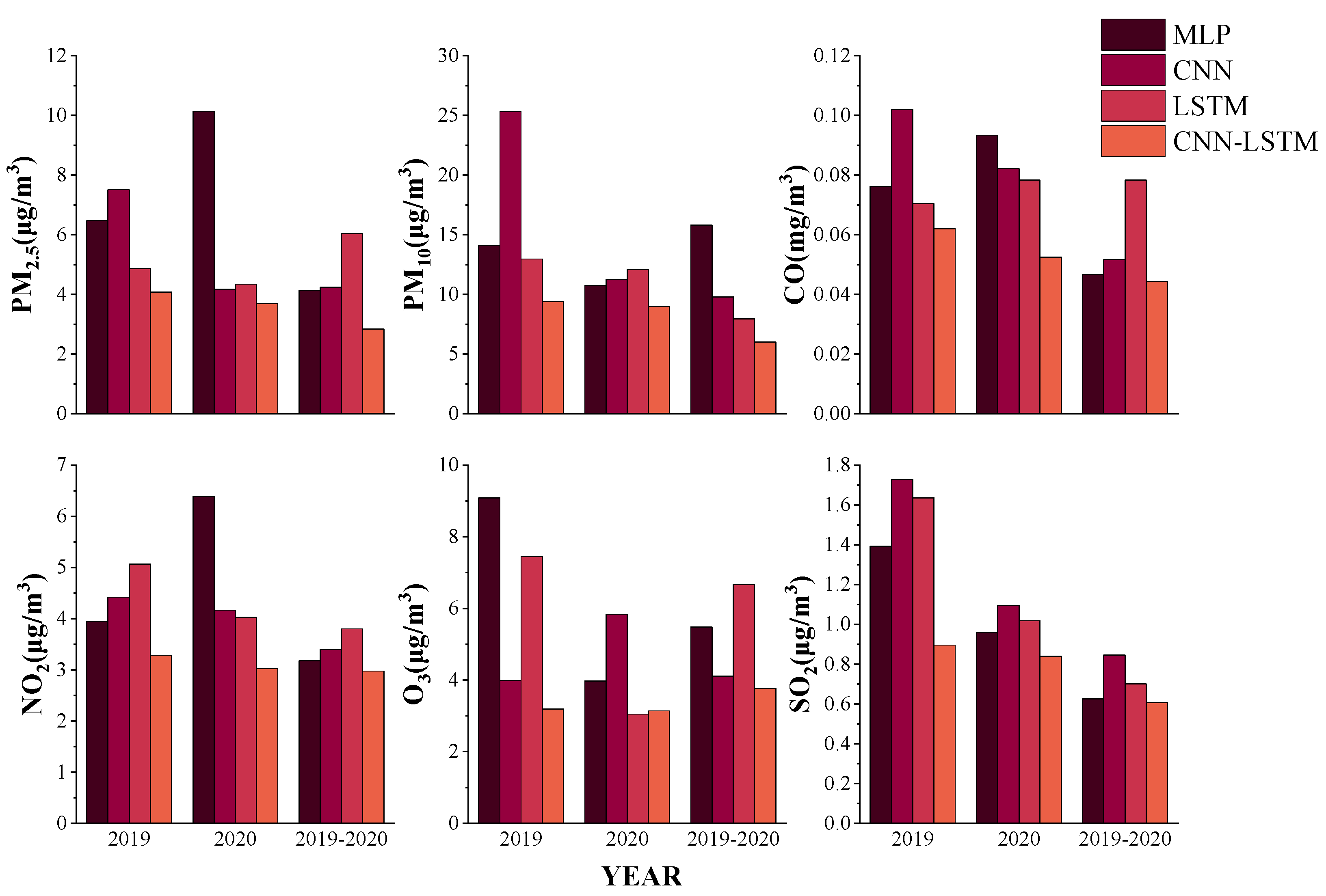
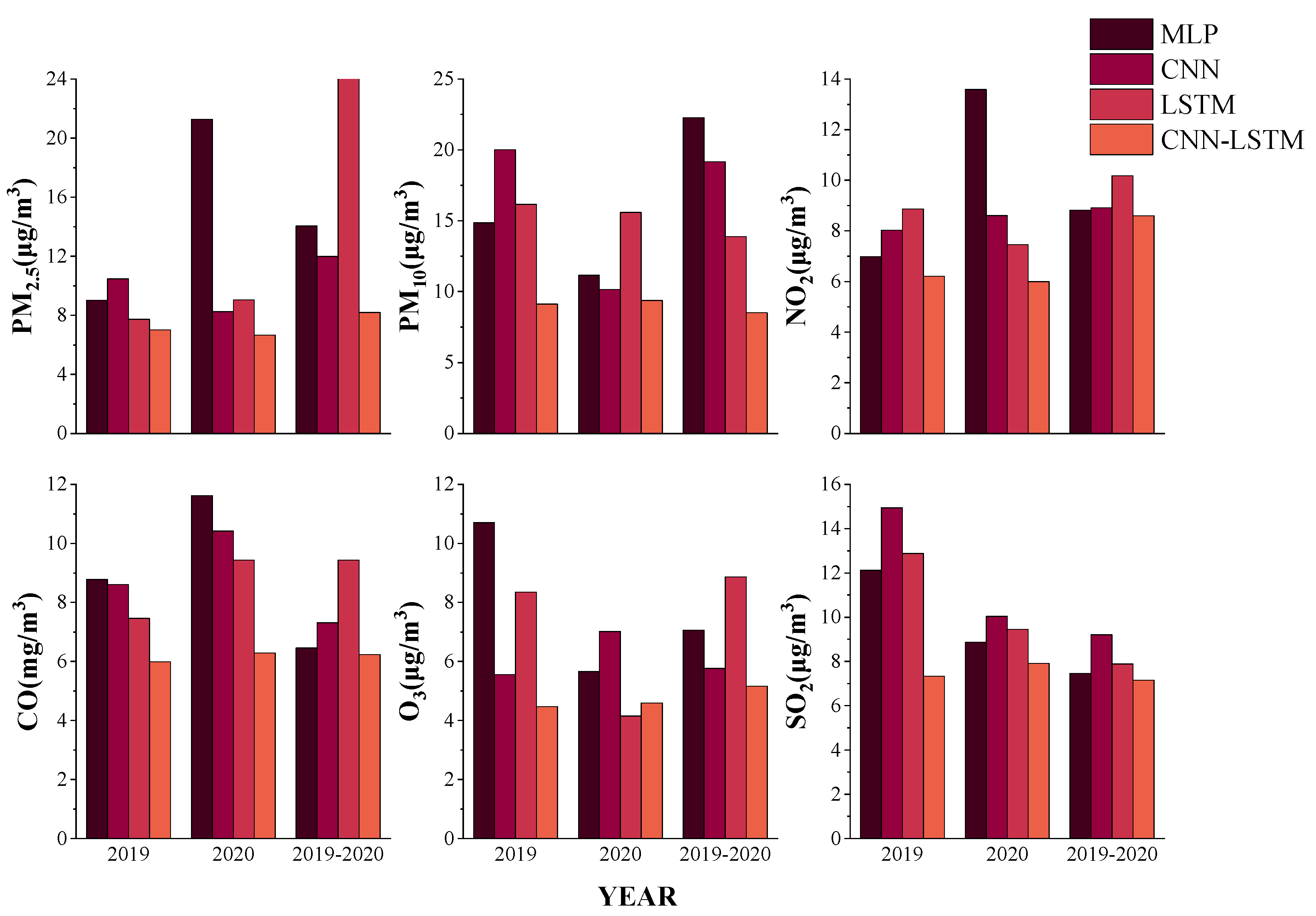
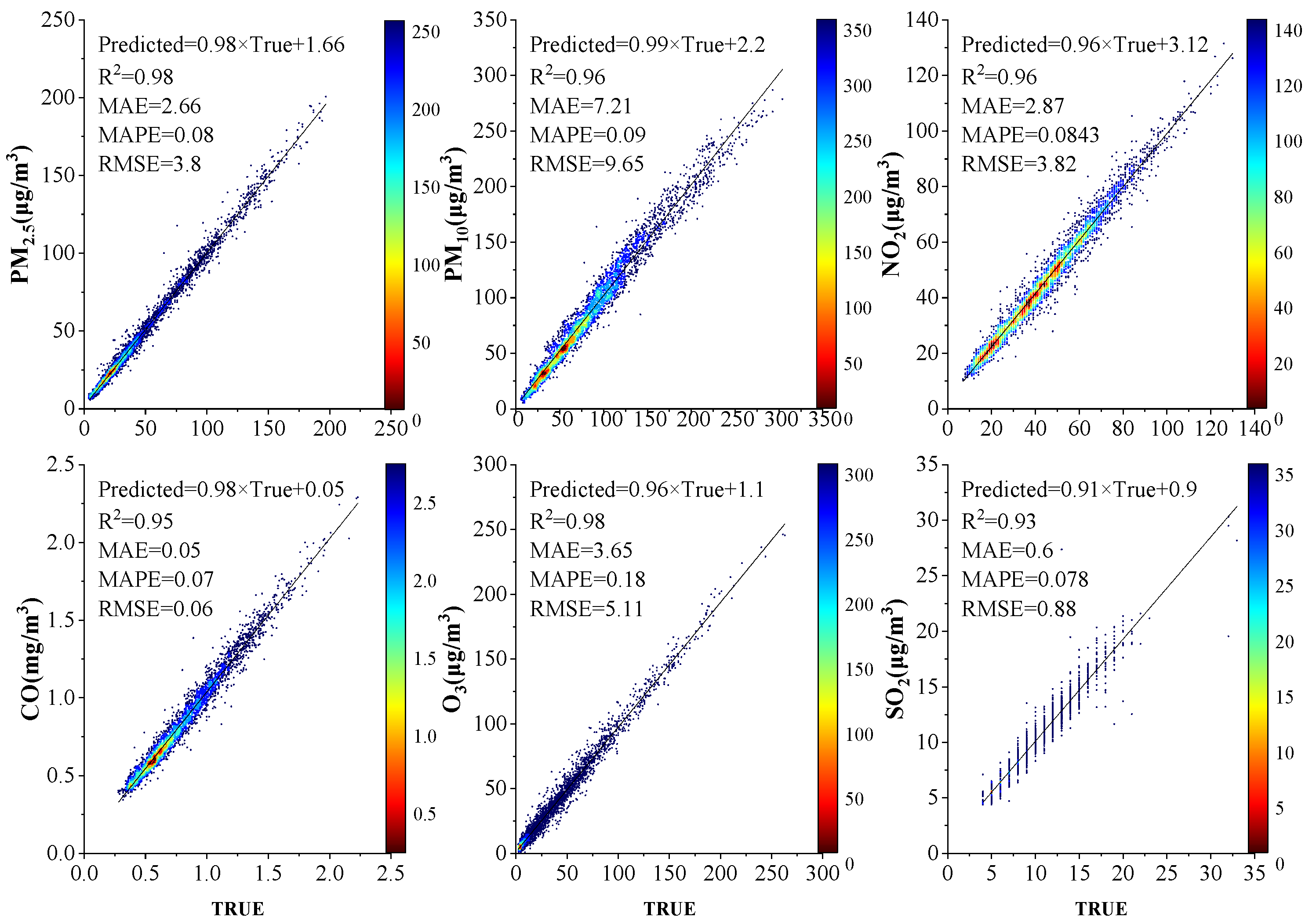
4.3. Grouped Data Comparison
According to the above research, it is found that the overall accuracy and error of the hourly data of air pollutants are better than those of the daily concentration data. Therefore, in order to test the performance of ODMSCNN-LSTM in the hourly concentration prediction, the grouped data comparison method is used to divide all the data into three groups to jointly verify the model. The first group of data includes the data set from 1 January 2019 to 31 December 2019, the second group of data consists of the data set from 1 January 2020 to 31 December 2020, and the third group uses data set from 1 January 2020 to 31 December 2020. The three groups of data are divided into the training set, validation set, and test set according to the ratio of 6:2:2. Additionally, the training set data is used to verify the prediction effect of each group of data.
The study found that the prediction performance of the same data in every model is different. In terms of prediction performance, the accuracy of the first group and the overall prediction performance of the training and validation sets are sorted in ascending order of MLP, CNN, LSTM, and ODMSCNN-LSTM. The prediction accuracy of the second group is MLP, CNN, LSTM, and ODMSCNN-LSTM from low to high. The accuracy of the third group is slightly different, arranged in ascending order of MLP, CNN, ODMSCNN-LSTM, and LSTM. Compared with the prediction performance of overall data set in the third group, the first and the second group have similar patterns with the overall prediction model. Using four deep learning models for training and verification of prediction accuracy, the results show that ODMSCNN-LSTM has the highest prediction accuracy on most test sets, and its prediction performance is better than other models for verification.
As shown in
Figure 9,
Figure 10 and
Figure 11, the RMSE, MAE, and MAPE values of the six air pollutants in the four models are shown, respectively. The prediction performance of the same pollutant using different data sets is different in the same model. This study selects the best-performing ODMSCNN-LSTM as an example. RMSE and MAE of the four air pollutants PM
2.5, PM
10, CO and SO
2 are arranged in descending order of 2019, 2020, 2019–2020. The RMSE and MAE of O
3 are arranged in descending order of 2019, 2020, 2019–2020, and those of NO2 are arranged in descending order of 2020, 2019, 2019–2020. The four atmospheric pollutants MAPE, PM
10, CO, O
3, and SO
2 are arranged in descending order of 2019, 2020, and 2019–2020.
In general, there may be many reasons why the prediction performance of the daily concentration data set in 2019 is worse than that in 2020. The concentration of air pollutants in 2019 is usually higher and there is a large fluctuation, which may lead the prediction model to make underestimation or overestimation. Therefore, RMSE, MAE and MAPE increase in the annual data prediction. Relevant laws, regulations and policies formulated by the Chinese government and the Xi’an municipal government may be one reason for that. Another reason is that there are less company-made and man-made emissions since the outbreak of COVID-19. In 2020, the concentration of air pollutants decreased, the overall air quality became better, and the peak value fluctuated slower. The spatial variation of air pollutant data set in 2020 tends to be stable compared with that in 2019, so prediction on air pollutants in 2020 is relatively easier. Which may be the main reason for smaller error of data prediction in 2020. Another reason for the overall good performance of 2019–2020 data set is related with certain performance of the deep learning model, which reflects that the more the data, the better the performance.
4.4. Comparison of Multiple Factors
After comparing the daily concentration data and hourly concentration data from the four models, it is found that ODMSCNN-LSTM model is better than others in overall performance. In order to test the efficiency of the prediction ability of the ODMSCNN-LSTM model, this paper continues to use the test set data of hourly data concentration to explore the influence of different factors on the prediction of air pollutant concentration.
The air pollutant concentration in Xi’an is affected by multiple factors. In order to better verify the ODMSCNN-LSTM model, a prediction model for different influencing factors has been established. The ODMSCNN-LSTM model was compared with air pollutants, meteorological factors, and overall factors to further verify the influence of multiple factors on the effect of the prediction model. All the data can be divided into three categories according to the types of influencing factors. The first category is to forecast only when meteorological factors are added. In the second category, only air pollutants are added as influencing factors. The third type is the whole factor which includes the meteorological factor and the air pollutant factor at the same time.
The paper draws the prediction curve of air pollutant concentration under different factors.
Figure 12 shows the comparison between: the actual value and the predicted value obtained after adding meteorological factors, and
Figure 13 shows the comparison between the actual value and the predicted value obtained after adding the air pollutants, and
Figure 14 shows the comparison between the actual value and the predicted value obtained after adding both the meteorological factors and the air pollutants. It is found that the prediction with meteorological factors is less effective than the other two types. Prediction, with only meteorological factors added, is better than the other two types of prediction. Furthermore, the three index values of MAE, MAPE, and RMSE are lower. By comparing the three types of influencing factors, it is found that prediction accuracy varies with different air pollutants.
Different air pollutant models have different performances in reducing errors and improving the consistency of changes in different factors. Adding meteorological factors may not be able to effectively improve the prediction accuracy. The decrease in the number of features of different factors leads to a decrease in the overall data for model training, which may limit the prediction ability of ODMSCNN-LSTM. Taking into account the annual characteristics of the concentration of air pollutants, the prediction error may be related to the type of air pollutants and the degree of dispersion of the air pollutant concentration in different seasons.
5. Discussion
In this study, an air pollutant concentration prediction model based on ODMSCNN-LSTM was developed and compared with three deep learning methods. The results show that the ODMSCNN-LSTM model performs better overall, is more suitable for daily or hourly concentration data sets and performs better on hourly data sets. This research shows that, compared with other machine learning, deep learning is a more effective method for processing big data (especially spatio-temporal data). Combining spatio-temporal data and models can improve the performance of spatio-temporal data prediction to a certain extent but adding meteorological factors does not necessarily improve the prediction performance of air pollutants. The reduction in the number of features may also affect the performance of the model. The prediction method proposed in this paper is feasible for the hourly concentration data prediction of multiple pollutants, and the method can also be applied into the air pollutant concentration prediction in multiple locations. In terms of input variables, regular monitoring data from the China National Environmental Monitoring Center and China Meteorological Administration are used. In terms of modeling methods, deep learning algorithms are combined with spatial and temporal features.
The performance of different air pollutants in the ODMSCNN-LSTM model may be due to differences in driving factors, temporal and spatial features, model types, model structures, and model development methods. At the same time, the amount of data, the degree of dispersion and spatial correlation between the concentration of air pollutants may also affect the prediction performance of the model, so it is necessary to further analyze the reasons for the difference. In addition, other factors, such as the increased output in equipment manufacturing, automobile manufacturing, electric power, heat production, gas and other industries, and the passenger and freight volume of the transportation industry need to be added in the follow-up research.


