Bias Correction for Precipitation Simulated by RegCM4 over the Upper Reaches of the Yangtze River Based on the Mixed Distribution Quantile Mapping Method

Abstract

Traditional multi-parameter single distribution quantile mapping (QM) methods excel in some respects in correcting climate model precipitation, but are limited in others. Multi-parameter mixed distribution quantile mapping can potentially exploit the strengths of single distribution methods and avoid their weaknesses. The correction performance of mixed distribution QM methods varies with the geographical location they are applied to and the combination of distributions that are included. This study compares multiple sets of single distribution and multi-parameter mixed distribution QM methods in order to correct the precipitation bias in the upper reaches of the Yangtze River basin (UYRB) in RegCM4 simulated precipitation. The results show that, among the selected distributions, the gamma distribution has the highest performance in the basin; explaining more than 50% of the precipitation events based on the weighting coefficients. The Gumbel distribution had the worst performance, only explaining about 10% of the precipitation events. The performance parameters, such as the root mean square error (RMSE) and the correlation coefficient (R) of the corrected precipitation, that were derived by using mixed distribution were better than those derived by using single distribution. The QM method that is based on the gamma-generalized extreme value distribution best corrected the precipitation, could reproduce the annual cycle and geographical pattern of observed precipitation, and could significantly reduce the wet bias from the RegCM4 model in the UYRB. In addition to enhancing precipitation climatology, the correction method also improved the simulation performance of the RegCM4 model for extreme precipitation events.

1. Introduction

Climate models are essential tools for studying climate change at global and regional scales. However, the regional climate model (RCM) and global climate model (GCM) typically have biases in the simulation of various climate variables (e.g., precipitation or temperature) when compared to the previously observed data, especially in mountainous areas [1,2]. In addition to the errors that are inherited from the driving data, there are also systematic model errors, due to imperfect conceptualization and parameterization, inadequate length and quality of reference data sets, and insufficient spatial resolution [3,4]. Such biases in simulating climate variables from climate models not only affect the assessment of future climate change effects, especially for extreme events, but also undermine the direct applicability of climate models to hydrology in the current and future climates [5,6,7]. Therefore, bias correction is generally required before climate simulation results from an RCM and a GCM for hydrology are applied.

Conventional correction methods for climate variables from RCM include the Delta method [8], multiple linear regression method [9], local intensity scaling method [10], and the QM method [11,12,13,14]. Although most correction methods have excellent bias correction performances for the mean climatology of climate variables, bias correction for statistical characteristics such as standard deviation and probability density need to be improved [15]. Themeßl et al. [14] compared numerous methods for correcting precipitation bias in climate models. They found that the QM method has the best overall bias correction performance for precipitation that is simulated by RCMs, especially in improving the simulation’s performance for extreme precipitation events. Tong et al. [2] and Han et al. [16] used the non-parametric RQUANT QM method to correct precipitation and temperature as simulated by RegCM4 for China, obtaining good bias correction results.

Studies have shown that the non-parametric QM method can effectively correct multiple biases in current climate variables simulated by RCMs and GCMs, but its correction effect is limited by the existing observed data and it has specific limitations for extreme climate events beyond observation [5,14]. Therefore, the QM method that is based on the multi-parameter statistical distribution (e.g., exponential distribution, gamma distribution and Weber distribution) has been widely used to correct the biases of climate variables from RCMs and GCMs [11,17,18]. However, the QM method that is based on multi-parameter single distribution still has limitations in correcting the biases. For example, the Weber distribution has a good correction performance for extreme events, but it is not ideal for general climate events. The exponential and gamma distributions have good correction effects for general climate events, especially for precipitation simulated by climate models. However, due to the light tail characteristics of these two distributions, the correction effects of extreme climate events predicted by climate models utilizing them are poor [11,13].

Mixture distribution has been widely used in precipitation and flood frequency analysis [13,19,20,21]. Teng et al. [20] compared the performance of four bias correction methods on RCM precipitation and found that the distribution mapping that was based on double gamma distribution could simultaneously capture Australian normal precipitation values as well as the extremes. Shin et al. [13] compared four sets of mixed distributions and found that heterogeneous mixture distributions performed the best in correcting precipitation biases in Korea, especially for extreme precipitation. Although heterogeneous mixture distributions can effectively correct the precipitation simulated by climate models, the large difference in precipitation structure across different regions and the diverse influences of extreme precipitation events make the same distribution not necessarily as effective in these regions. This inevitably requires a study on the adaptation of the mixed distribution of precipitation in a specific area in order to determine the best distribution [22].

The model-simulated precipitation for the upper reaches of the Yangtze River basin (UYRB) differs substantially from the observations, due to the region’s complex precipitation-producing weather systems and terrains. To overcome the limitations of the traditional QM method that is based on the multi-parameter single distribution, we used the multi-parameter binary mixed distribution QM method in order to correct the precipitation biases simulated by the RegCM4 model for the UYRB. The performance of bias correction for precipitation using the QM method that is based on different mixed distributions was evaluated using observation. Based on the performance evaluation results of the precipitation bias correction, the mixed distribution function with the best performance was able to be determined for the UYRB RegCM4 simulation. In addition, the correction performance for extreme precipitation indices was evaluated. The results can provide guidance for using the mixed distribution QM method in order to correct the precipitation predicted for the UYRB in similar regional climate models.

2. Materials and Methodology

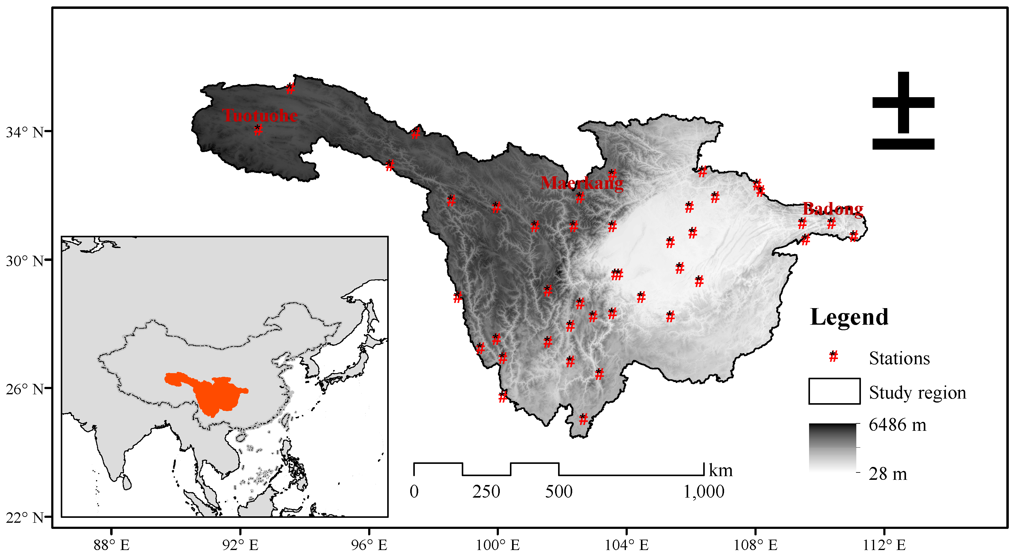
2.1. Study Area

This study defines the UYRB as the Yangtze River basin (YRB) above Yichang in Hubei province. The area and runoff of the UYRB account for 59% and 46% of the YRB, respectively (Figure 1). The precipitation in the UYRB is subject to the comprehensive influence of the East Asian summer monsoon and south Asian summer monsoon all year round [23]. The summer precipitation in the basin accounts for more than 80% of the total amount of annual precipitation and summer flooding disasters are frequent [24,25]. Due to the highly variable terrain and regional climates and complex precipitation mechanisms in the UYRB, the simulation performance of RCMs and GCMs for precipitation in this region is generally poor. Because it is challenging to apply simulation results to hydrology and other impact studies, the modeled precipitation needs to be corrected for biases.

2.2. Precipitation Data

The data used in this study include precipitation data sets from a RegCM4 simulation and observational data sets. The precipitation that has been simulated by RegCM4 for the period from 1989 to 2012 was based on the model configuration scheme from Huang et al. [26]. In addition, the EAR-Interim reanalysis data were used as initial and boundary conditions to perform dynamic downscaling with a resolution of 50 km. The detailed model configuration is shown in

Table 1. The RegCM4 model configuration used in this study.

Contents	Description
Domain	50 km horizontal resolution Central Lat. and Lon.: 35° N, 115° E 200 (Lon) × 130 (Lat)
Vertical layers (top)	18 vertical sigma levels (1 hPa)
PBL scheme	Holtslag
Cumulus parameterization scheme	Emanuel
Land surface model	NCAR CLM3.5
Short-/Longwave radiation scheme	NCAR CCM3
Boundary data	EAR-Interim reanalysis data
Simulation period	January 1989–December 2012

.

The daily precipitation observations derived from 42 meteorological stations in the UYRB from 1961–2015 (

Table 2. Meteorological stations used in the study.

ID	Name	Lat (°)	Lon (°)	ID	Name	Lat (°)	Lon (°)
52908	Wudaoliang	35.3	93.6	56565	Yanyuan	27.4	101.6
56004	Tuotuohe	34	92.6	56571	Liangshan	27.9	102.3
56029	Yushu	32.9	96.7	56651	Lijiang	26.9	100.2
56034	Qingshuihe	33.9	97.5	56671	Huili	26.8	102.3
56144	Dege	31.8	98.6	56684	Huize	26.4	103.2
56146	Ganzi	31.6	100	56751	Dali	25.7	100.2
56167	Daofu	31	101.2	56778	Kunming	25	102.7
56172	Maerkang	31.9	102.6	57211	Ningqiang	32.7	106.4
56178	Xiaojing	31	102.4	57237	Wanyuan	32.1	108.2
56182	Songpan	32.6	103.6	57238	Zhenba	32.3	108.1
56188	Dujiangyan	31	103.6	57306	Langzhong	31.6	106
56385	Emeishan	29.5	103.7	57313	Bazhong	31.9	106.8
56386	Leshan	29.5	103.8	57348	Fengjie	31.1	109.5
56444	Deqin	28.8	98.8	57355	Badong	31.1	110.4
56462	Jiulong	29	101.6	57405	Suining	30.5	105.4
56475	Yuexi	28.6	102.6	57411	Nanchong	30.8	106.1
56479	Zhaojue	28.2	103	57445	Jianshi	30.6	109.6
56485	Leibo	28.3	103.6	57461	Yichang	30.7	111.1
56492	Yibin	28.8	104.5	57502	Dazu	29.7	105.7
56543	Diqing	27.5	100	57517	Jiangjin	29.3	106.3
56548	Weixi	27.2	99.5	57608	Xuyong	28.2	105.4

) and the gridded observation analysis data set CN05 [27] were used to evaluate the bias corrections. The CN05 data set is produced by the China Meteorological Administration using the anomaly approximation method to interpolate the observation data of more than 2400 national meteorological stations into a 0.25° × 0.25° grid. The precipitation that was simulated by RegCM4 was interpolated into the CN05 grid by using bilinear interpolation to compare the simulation with the observed data. To demonstrate the robustness of the QM method used in this study in different areas of the UYRB, we selected three stations from the eastern, central and western parts of the basin; namely Badong, Maerkang and Totohe. Badong is located in the southwestern part of Hubei Province (110.4° E, 31.1° N), in the subtropical monsoon area, with an average annual precipitation amount of more than 1000 mm. Located in the northwest of Sichuan Province (102.6° E, 31.9° E), Maerkang has a plateau continental monsoon climate with an annual precipitation amount of about 700 mm. Tuotuohe, located in western Qinghai Province (92.6° E, 34° N) on the Tibetan Plateau, is characterized by a plateau continental climate with scarce precipitation.

2.3. Mixed Distribution QM

The traditional QM method adjusts the probability distributions of the climate variables simulated by the RCM to those of the observation, so that the cumulative probability density functions (CDFs) of the observation and the simulated CDFs are consistent. The corrected climate variables can be obtained by mapping the CDFs of the climate variables simulated by the climate models to the corresponding observation data (OBS) CDFs using the QM method. A basic assumption of this method is that the climate distribution will not change greatly over time; that is, the variance and skewness of the distribution are stable and only the mean changes [28]. The traditional QM method is defined as:

$$y=F_{obs}^{-1}\left(F_{RCM}\left(x\right)\right)$$

(1)

where $F_{obs}^{-1}$ represents the inverse function of the CDF of the observed climate elements and $F_{RCM}$ represents the CDF of the output data from the RCM. The mixed distribution QM method that uses multiple distribution functions is defined as follows:

$$f\left(x\right)={\displaystyle \sum }_{i=1}^n{\sigma }_i{f}_i\left(x; {\delta }_i\right)$$

(2)

where ${\delta }_i$ is a parameter of the i_th distribution function; ${\sigma }_i$ is the weight coefficient of the distribution component; and n is the number of mixed distribution components. Due to the complexity of the multi-parameter mixed distribution model, which requires many computing resources, only the multi-parameter binary mixed distribution model is analyzed. Thus, the number of mixed distribution components set in the study is two.

Multi-parameter single distribution functions such as gamma distribution (G), exponential distribution (E), generalized extreme value distribution (GEV, V), and Gumbel distribution (U) were selected as they have been widely used in hydrometeorological research and have shown good performance [13,20,29,30]. Then, we set four mixed distributions: G-G, G-E, G-V, and G-U. The mixed distribution functions are expressed as follows:

$$f_{G\text{-}G}\left(x; {\alpha }_1, {\beta }_1,{\alpha }_2, {\beta }_2\right)=\sigma f_G\left(x; {\alpha }_1, {\beta }_1\right)+\left(1-\sigma \right)f_G\left(x; {\alpha }_2, {\beta }_2\right)$$

(3)

$$f_{G\text{-}E}\left(x; {\alpha }_1, {\beta }_1,{\alpha }_2\right)=\sigma f_G\left(x; {\alpha }_1, {\beta }_1\right)+\left(1-\sigma \right)f_E\left(x; {\alpha }_2\right)$$

(4)

$$f_{G\text{-}V}\left(x; {\alpha }_1, {\beta }_1,{\alpha }_2, {\beta }_2,\gamma \right)=\sigma f_G\left(x; {\alpha }_1, {\beta }_1\right)+\left(1-\sigma \right)f_V\left(x; {\alpha }_2, {\beta }_2, \gamma \right)$$

(5)

$$f_{G\text{-}U}\left(x; {\alpha }_1, {\beta }_1,{\alpha }_2, {\beta }_2\right)=\sigma f_G\left(x; {\alpha }_1, {\beta }_1\right)+\left(1-\sigma \right)f_U\left(x; {\alpha }_2, {\beta }_2\right)$$

(6)

The RegCM4 simulation generally produced more precipitation events than the observation. This is because the precipitation frequency in RegCM4 was bias corrected to the observed precipitation events (measured in days) per month by generating a new daily precipitation series that matched the probability of zero daily precipitation. The probability (P₀) of zero daily precipitation observations is defined as:

$$P_0^{obs}=n_0^{obs}/N_{}^{obs}$$

(7)

where $N_{}^{obs}$ is the total number of days in the reference period and $n_0^{obs}$ is the dry days in $N_{}^{obs}$. The zero events of observed precipitation are generally larger than those of daily precipitation simulated by RegCM4, i.e., $P_0^{RCM}<P_0^{obs}$. Therefore, some light precipitation events should be treated as zero-value events so that the observed and simulated zero-value events have the same occurrence probability:

$$x=\{\begin{array}{c}{x}_{RCM} x_{RCM>\varnothing }\\ 0 x_{RCM\le \varnothing }\end{array}$$

(8)

where $\varnothing$ is the threshold to satisfy $P_0^{RCM}=P_0^{obs}$ in the RegCM4 model.

In this study, the genetic algorithm was used to automatically optimize the parameters of the distribution function for all grid points and meteorological stations. To quickly determine the parameters of the distribution function, we used the observed value to calculate the 95% confidence interval of the maximum likelihood estimate of a single distribution parameter and then combined the effective range of each parameter in the distribution function in order to determine the parameter optimization calculation interval (except for weight coefficient (${\sigma }_i$). The mean relative error (MRE) and correlation coefficient (R) were used to construct the genetic algorithm optimization objective function. At the same time, the root mean square error (RMSE) and error sum of squares (SSE) were also combined in order to evaluate the fitting performance. In this study, the maximum number of iterations of the genetic algorithm was 300, the objective function convergence tolerance was 10⁻⁵, and the iteration step convergence tolerance was 10⁻⁶.

2.4. Analysis Methods

The Kolmogorov-Smirnov (K-S) statistical test was used to evaluate the fitting performance of the different mixed distributions to the observed precipitation that was sourced from 42 meteorological stations. Based on the evaluation results, the optimal distribution function for the UYRB precipitation biases’ correction was determined. D is defined as the maximum difference between F₀(x) and F_n(x) as follows:

$$D=\underset{-\infty <x<\infty }{\max }\left|F_n\left(x\right)-F_0\left(x\right)\right|$$

(9)

where F_n(x) is an empirical distribution function and F₀ (x) is the assumed population distribution function; if D > D_a, accept H₁, otherwise, accept H₀; P₉₅ is the number of meteorological stations that pass the 95% confidence level of the K-S test.

To evaluate the bias correction performance for extreme precipitation events, the consecutive dry days (CDD), simple daily intensity index (SDII), very wet day precipitation (R_90th), and very wet days (PN_90th) were selected and analyzed. The CDD measure was defined as the maximum number of consecutive days with daily precipitation amounting to less than 1 mm in a year. The SDII was defined as the annual total amount of precipitation divided by the number of wet days in a year. R_90th and PN_90th were defined as precipitation of the 90th quantile and the count of days when precipitation exceeds R_90th, respectively.

3. Results

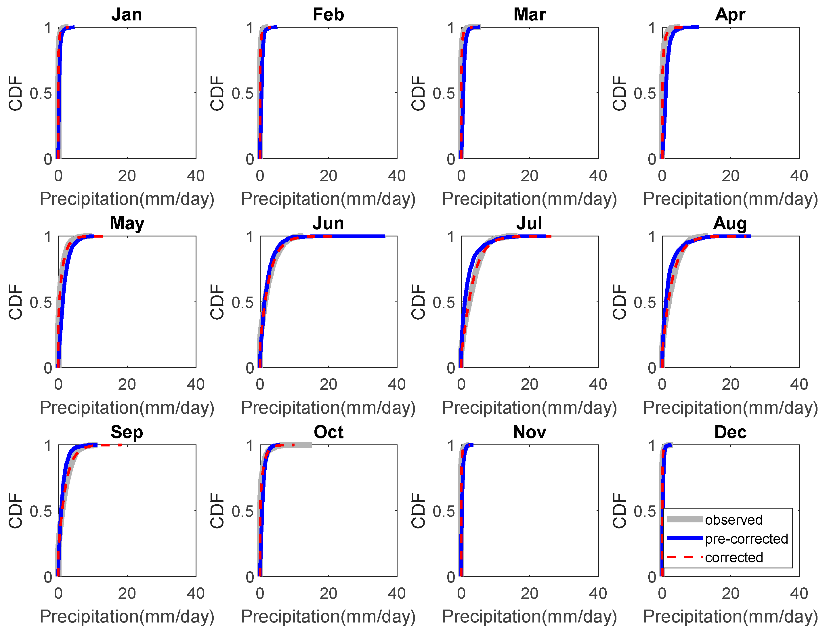
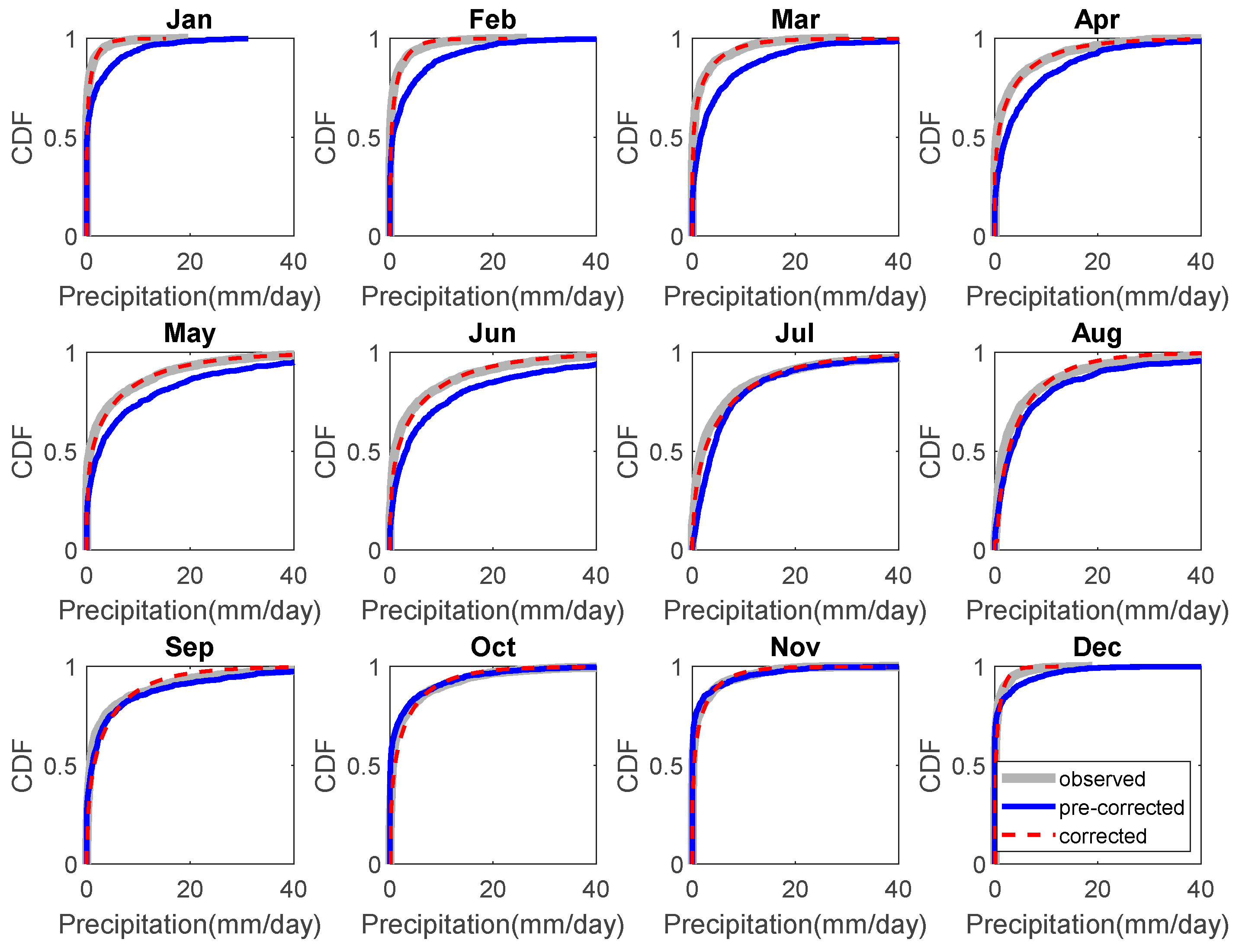
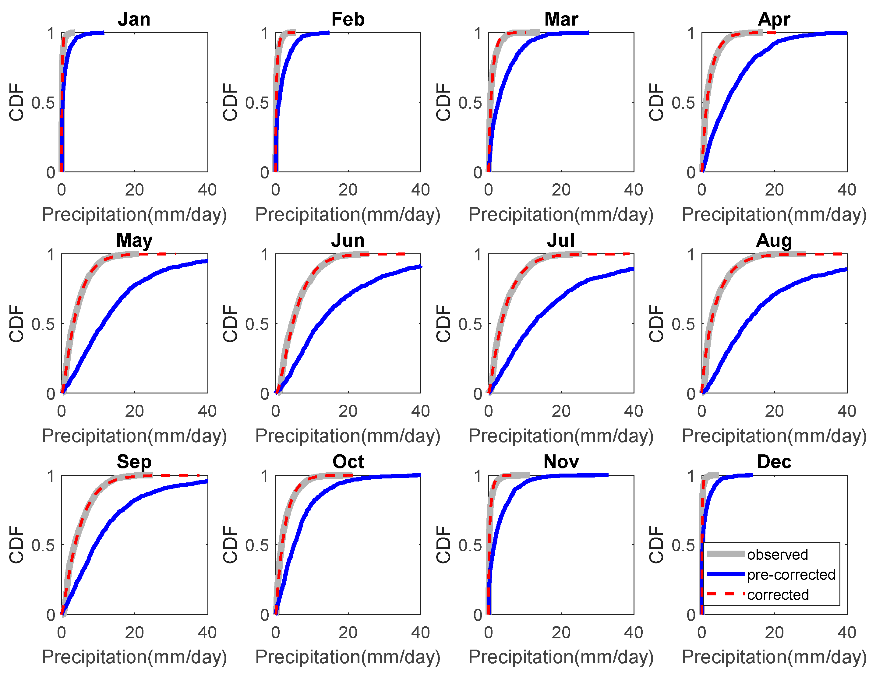
3.1. Correction Performance of Different Distribution Functions

Based on the performances of the four selected single distributions, G (gamma distribution) and V (GEV distribution) were found to be more applicable to the UYRB than E (exponential distribution) and U (Gumbel distribution) were, when used alone. However, even with the best G distribution, only 23 stations passed the K-S test, indicating that single distribution has apparent limitations in precipitation fitting for the UYRB. To evaluate the fitting performance of four single and four mixed distributions to historically observed precipitation in the UYRB, daily observed precipitation was selected from 42 meteorological stations in the basin (data were collected from observations taking place from 1961 to 2015). According to

Table 3. Comparison of fitting performance between single distribution and mixed distribution.

Distribution Function	K-S Statistical Parameter		MRE	RMSE	SSE	R
	D	P95
G	0.32	23	20.59	6.87	1.66	1.00
E	0.54	8	54.90	27.08	22.74	0.98
U	0.80	0	164.92	43.75	63.23	0.94
V	0.38	14	9.32	13.44	6.01	0.99
G-G	0.18	38	1.17	1.39	0.16	1.00
G-E	0.19	40	−1.26	1.35	0.18	1.00
G-U	0.37	13	8.10	3.17	0.38	1.00
G-V	0.17	39	−1.07	1.29	0.14	1.00

, the D of U (Gumbel distribution) was 0.8 and no sites passed the K-S test (P₉₅ = 0). The MRE, RMSE, SSE, and R were 164.92, 43.75, 63.23, and 0.94, respectively. Compared with U distribution, the statistics D, MRE, RMSE, SSE, and R of the G distribution, E distribution, and V distribution were significantly lower than those of the U distribution. At the same time, the P₉₅ and R of these single distributions (G, E, V) were also higher than the U distribution.

The mixed distribution significantly outperformed the four selected single distributions for fitting the observed precipitation distribution in the UYRB. With the combination of the U distribution and G distribution, the fitting performance of G-U improved as the parameters D, MRE, RMSE, and SSE decreased significantly and the number of sites passing the K-S test (P₉₅) increased from 0 to 13. However, of the four mixed distributions, the fitting performance of the G-U distribution was still the worst, indicating that the U distribution is not suitable for precipitation fitting in the UYRB. Multi-parameter binary mixed distribution functions, such as G-G, G-E, and G-V, have significantly better fitting performances for observed precipitation than their corresponding single distribution functions. Compared with other single distributions, the single distributions of G and V had better fitting performances for observed precipitation over the UYRB. Specifically, the G-V mixed distribution, comprising the two optimal single distributions (G and V), performed better than the corresponding single distributions and was superior to other mixed distributions. The D, MRE, RMSE and SSE of the G-V mixed distribution were the least compared with those of the other mixed distributions, indicating that the G-V mixed distribution had the best performance. In addition, the P₉₅ of the G-V mixed distribution reached 39, i.e., more than 93% of the UYRB stations passed the K-S test, further indicating that the G-V mixed distribution had excellent fitting performance for the observed precipitation in the basin. Therefore, the QM method that is based on the binary mixed G-V distribution was the most suitable for correcting the daily precipitation biases simulated by RegCM4 for the UYRB.

The performance of the G distribution in the UYRB was more robust than those of the other three single distributions, while the performance of U was the poorest. The precipitation types of 42 meteorological stations in the UYRB can be represented by the weighting parameter (σ) of the binary mixed distribution function for further interpretation (Figure 2). The median gamma distribution parameters in G-G, G-E, G-V, and G-U mixed distributions were about 0.5, 0.7, 0.8, and 0.9, respectively. The σ parameters of the G distribution component indicated that more than 50% of precipitation events in the UYRB conformed to the G distribution’s characteristics and could be explained by the G distribution. In comparison, the U distribution could only explain less than 10% of precipitation events in the basin.

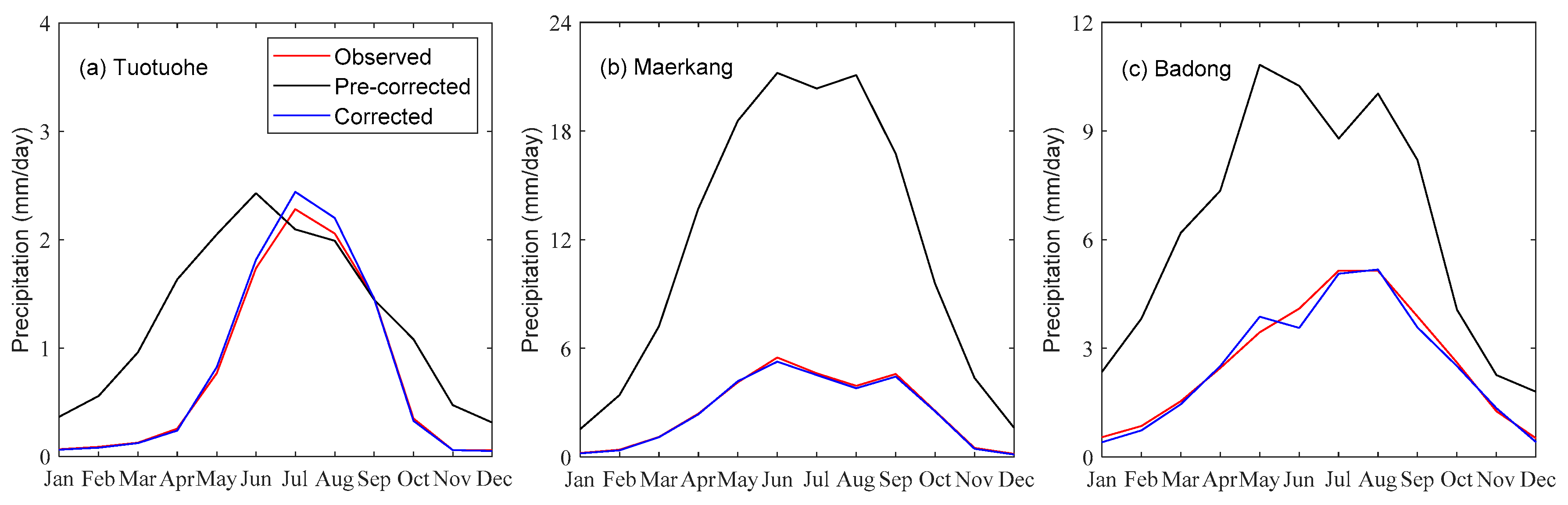
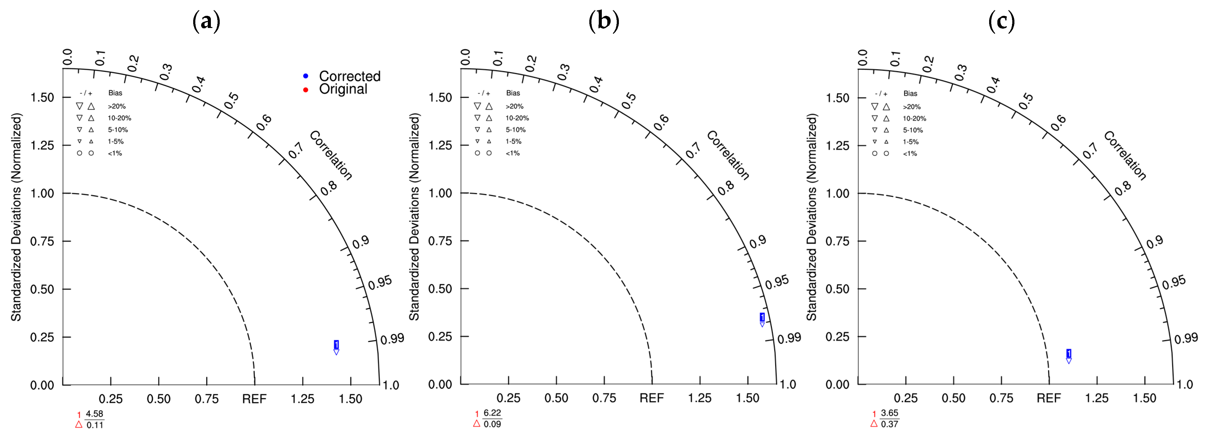
3.2. Correction Performance for Station Precipitation

After the QM method was applied based on the binary mixed G-V distribution on daily precipitation, the precipitation CDF in each month was closer to that of the observation. In particular, the wet bias of the CDF above 0.9 was substantially reduced. The CDFs of Tuotuohe (Figure 3) and Badong (Figure 4), after correction, were consistent with the CDF of the observed precipitation. As shown in Figure 3, Figure 4 and Figure 5, the biases between the modeled precipitation CDF and observed precipitation CDF at Totohe were the smallest, followed by Badong. The biases between the observed precipitation CDF and the originally modeled CDF are the largest at Maerkang, especially from March to September.

As shown in Figure 6, the QM method that is based on the binary mixed G-V distribution gave a good performance for bias correction for the CDF and annual precipitation cycle in the eastern, central, and western UYRB as simulated by RegCM4. The binary mixed G-V distribution had strong adaptability and robustness to precipitation bias correction at different meteorological stations in the UYRB. The multi-year average monthly maximum precipitation observed at Totohe was about 1.8 mm/day in June, while before bias correction, it was in May (about 2.4 mm/day). The multi-year average monthly maximum precipitation at Maerkang was in June, when it was observed at 5.3 mm/day and simulated at 21.2 mm/day (before bias correction). Before bias correction, the annual precipitation cycle in Badong showed a bimodal pattern, with the multi-year average monthly maximum precipitation exceeding 10 mm/day in May and August. However, the observed annual precipitation cycle had a single peak, with the multi-year average monthly maximum precipitation at a rate of only 3.8–5mm/day. Compared with the observed data, the annual precipitation cycles in Totohe, Maerkang, and Badong before bias correction deviated substantially from the actual precipitation cycles, especially in Totohe and Badong. After bias correction, the annual precipitation cycles were consistent with those that were observed, and the monthly wet biases were significantly reduced.

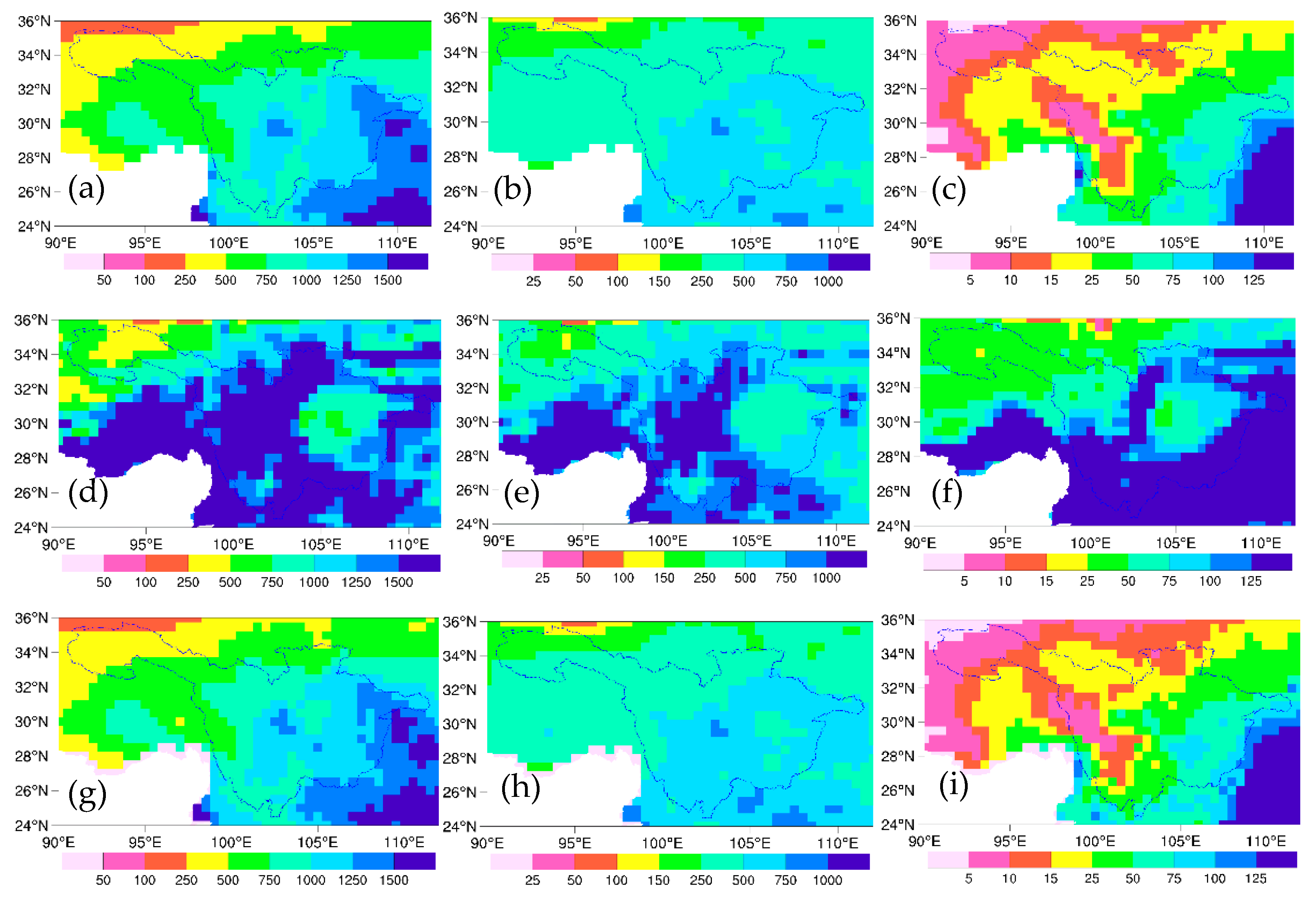
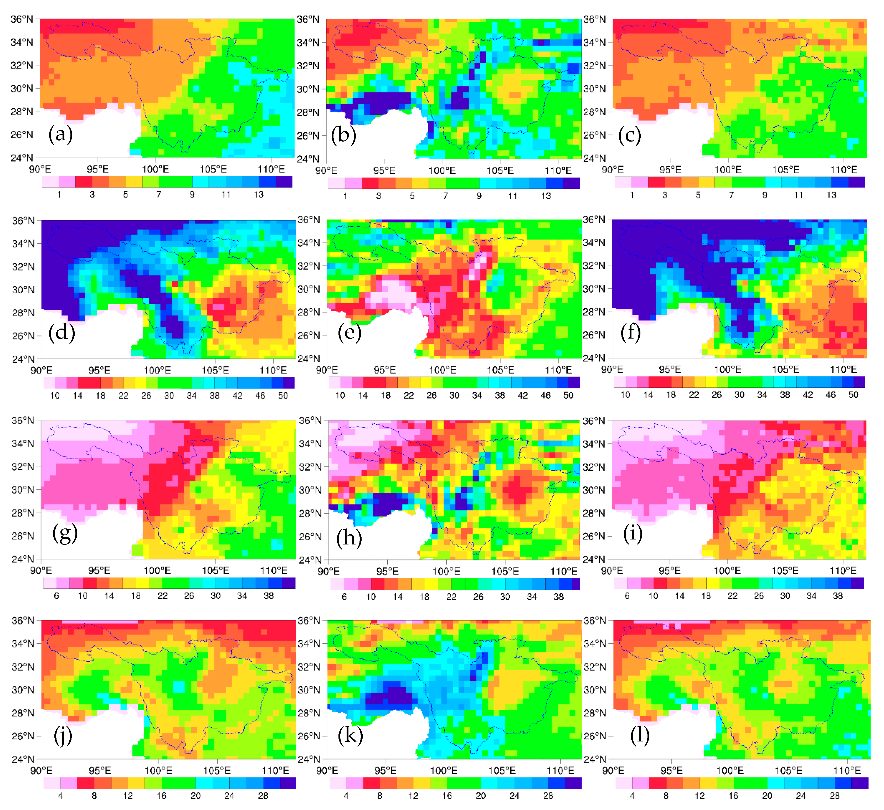
3.3. Correction Performance for Precipitation Climatology and the Extreme Precipitation Index

The performance of precipitation bias correction using QM methods that are based on the G-V mixed distribution was better for winter precipitation than for summer (Figure 7). As shown in Figure 7a, the spatial correlation coefficient of the precipitation between the simulated and observed scores before correction (marked in red) was only about 0.1. The simulation performance of RegCM4 for predicting winter precipitation was slightly better than predictions for summer. The spatial correlation coefficient of winter precipitation before correction was about 0.35, but the precipitation wet biases were generally more than 25%. After the precipitation bias correction, the spatial correlation coefficient of precipitation between the simulated and observed scores increased from 0.1 to 0.99. The precipitation wet biases decreased from 25% to about 10%.

After the bias correction, the precipitation wet biases that were simulated by RegCM4 for the UYRB were significantly reduced and the spatial distribution characteristics of annual mean, summer, and winter precipitation were all in agreement with the observed precipitation (Figure 8a–c,g–i), despite the bias correction being conducted with daily data. As shown in Figure 8a, the observed annual average precipitation in the eastern and central parts of the UYRB was over 1000 mm, while the annual average precipitation in the western part of the UYRB was generally less than 500 mm. Compared with the observed precipitation, there was a large wet bias in the precipitation from RegCM4, before the correction, relative to the observation, especially in the mountainous areas surrounding the Sichuan Basin (Figure 8d–f). The simulated annual precipitation over Songpan Plateau, Yunnan-Guizhou Plateau, and Wushan could be over 1500 mm, which was more than twice the corresponding observation, before correction. For seasonal precipitation, the summer and winter precipitation that was simulated by RegCM4 also had a sizeable wet bias when compared with the observed precipitation, which was mainly concentrated in mountainous areas with complex terrains.

The QM methods that are based on the G-V mixed distribution have good correction performance for precipitation climatology and extreme precipitation events. The observed, simulated, and corrected results of the SDII, CDD, R90th, and PN90th are presented (Figure 9). Due to the wet bias of the simulated precipitation, especially in the mountainous area, the predicted SDII, R90th, and PN90th were higher than the observed scores, while the number of CDD was lower (Figure 9b,e,h,k). As a result, the spatial correlation coefficient between the simulation and observation of the extreme precipitation indices was below 0.3. However, after bias correction, the spatial distributions of the SDII, CDD, R90th, and PN90th were very close to the observed scores and the spatial correlation coefficients all increased to above 0.9. (Figure 9c,f,i,l).

Notably, the bias correction for precipitation climatology and extreme precipitation indices is highly dependent on the observation data. In this study, the correction eliminated the precipitation wet bias in the mountain areas as simulated by the RegCM4 model, but the lack of observational precipitation data in the mountainous areas may have led to uncertainty in the correction of heavy precipitation events. Therefore, attention must be paid to the uncertainty of the observational data in precipitation bias correction. Heavy precipitation is often present in mountainous areas, such as the Tianshan Mountains, Kunlun Mountains, and the Yarlung Zangbo Grand Canyon in Tibet, but it is often not recorded [1,31]. In a similar study, Tong et al. [2] used a non-parametric QM to correct the precipitation that was simulated by RegCM4 and found that bias correction’s performance depends on the observed data.

4. Discussion and Conclusions

To better apply RegCM4-simulated precipitation in hydrological applications, bias correction of RegCM4-simulated daily precipitation was performed based on the QM method of mixed binary distribution with different multi-parameters. The QM methods using single distributions and mixed binary distributions on precipitation observations were compared. In addition, the bias correction results from the best performing distribution—the G-V mixed distribution—were analyzed.

Gamma distribution is often employed as a distribution model in the bias correction of precipitation [13,32]. The appropriateness of using the gamma distribution for modeling precipitation has been proven in an extensive body of literature [13,20,32,33]. As expected, out of the selected single distributions, the gamma distribution had the best performance in the UYRB, dominating the representation of precipitation distribution with a weighting coefficient more than 50% in the mixed distribution. In contrast, the Gumbel distribution had the worst performance, only explaining about 10% of the precipitation events, indicating that the Gumbel distribution is not suitable for fitting the precipitation distribution in the UYRB.

However, the gamma distribution alone was still not the best fit that was found in this study. The performances of the evaluations based on the D of the K-S test, RMSE, SSE, and R of precipitation corrected by mixed distribution are all better than those of single distribution, indicating that the QM method that is based on the multi-parameter binary mixed distribution has the best correction performance for regional climate model-simulated precipitation in the UYRB. Of the selected mixed distributions, the QM method that is based on the gamma-GEV distribution had the best performance for bias correction for precipitation in the basin by generating the closest CDFs. The gamma-GEV distribution was able to significantly reduce the precipitation wet bias that was simulated by the RegCM4 model. It also faithfully reproduced the observed annual cycles of precipitation and their geographical patterns. In addition, this distribution was able to improve the simulation performance of the RegCM4 model for extreme precipitation events. The good performance of the heterogeneous mixed distribution of gamma-GEV on the bias correction of extreme precipitation and normal precipitation has also been verified in South Korea [13]. In other regions, such as Thailand’s Upper Ping River Basin, both Bernoulli-Weibull and Bernoulli-gamma have good performances for precipitation bias correction [22], showing that the optimal choice of distributions is dependent on regional hydro-meteorological characteristics.

In general, the QM method that is based on the mixed binary distribution of gamma-GEV demonstrated a good performance for bias correction for the magnitude and spatial distribution of the precipitation simulated by the RegCM4 model over the UYRB. However, the mixed distribution still could not fit all of the observation sites in the basin well enough to pass the K-S test, which indicates there is still room for the method to be further optimized. On the other hand, the QM method that is based on the mixed binary distribution assumes a time-invariant bias (or transfer function) such as those present in other statistical downscaling techniques [2,13,28]. However, more and more evidence shows that the current global hydrological cycle is intensifying, which may cause this hypothesis to be untenable under the severe impact of climate change [34,35]. For example, if the region of interest experiences a different rainfall regime in the future as a result of changes in large-scale circulation, then the future bias would be controlled by different processes and the behavior of the bias may change. This is a limitation of the method used in the present study and one that should be borne in mind as we deal with future projections.

In future studies, we will identify regions that need further investigation and explore the effects of the QM method that is based on the mixed ternary distribution. We will also add time-varying parameters into the bias correction model in order to provide reliable precipitation data sets from regional climate downscaling for better climate change impact assessment and risk analysis.

References

1. Gao, X.-J.; Shi, Y.; Han, Z.-Y.; Wang, M.-L.; Wu, J.; Zhang, D.-F.; Xu, Y.; Giorgi, F. Performance of RegCM4 over Major River Basins in China. Adv. Atmos. Sci. 2017, 4, 441–455. [Google Scholar] [CrossRef]
2. Tong, Y.; Gao, X.-J.; Han, Z.-Y.; Xu, Y. Bias Correction of Daffy Precipitation Simulated by RegCM4 Model over China. Chin. J. Atmos. Sci. 2017, 6, 1156–1166. (In Chinese) [Google Scholar]
3. Jie, C.; Brissette, F.-P.; Leconte, R. Uncertainty of downscaling method in quantifying the impact of climate change on hydrology. J. Hydrol. 2011, 401, 190–202. [Google Scholar]
4. Piani, C.; Weedon, G.-P.; Best, M.; Gomes, S.-M.; Viterbo, P.; Hagemann, S.; Haerter, J.-O. Statistical bias correction of global simulated daily precipitation and temperature for the application of hydrological models. J. Hydrol. 2010, 395, 199–215. [Google Scholar] [CrossRef]
5. Haddeland, I.; Heinke, J.; Voß, F.; Eisner, S.; Chen, C.; Hagemann, S.; Ludwig, F. Effects of climate model radiation, humidity and wind estimates on hydrological simulations. Hydrol. Earth Syst. Sci. 2012, 16, 305–318. [Google Scholar] [CrossRef] [Green Version]
6. Hagemann, S.; Chen, C.; Haerter, J.-O.; Heinke, J.; Gerten, D.; Piani, C. Impact of a Statistical Bias Correction on the Projected Hydrological Changes Obtained from Three GCMs and Two Hydrology Models. J. Hydrometeorol. 2011, 4, 556–578. [Google Scholar] [CrossRef]
7. Piani, C.; Haerter, J.-O.; Coppola, E. Statistical bias correction for daily precipitation in regional climate models over Europe. Theor. Appl. Climatol. 2010, 1, 187–192. [Google Scholar] [CrossRef] [Green Version]
8. Navarro-Racines, C.; Tarapues, J.; Thornton, P.; Jarvis, A.; Ramirez-Villegas, J. High-resolution and bias-corrected CMIP5 projections for climate change impact assessments. Sci. Data 2020, 7, 7. [Google Scholar] [CrossRef] [Green Version]
9. Ibarra-Berastegi, G.; Saénz, J.; Ezcurra, A.; Elías, A.; Diaz Argandoña, J.; Errasti, I. Downscaling of surface moisture flux and precipitation in the Ebro Valley (Spain) using analogues and analogues followed by random forests and multiple linear regression. Hydrol. Earth Syst. Sci. 2011, 6, 1895–1907. [Google Scholar] [CrossRef]
10. Willkofer, F.; Schmid, F.; Komischke, H.; Korck, J.; Braun, M.; Ludwig, R. The impact of bias correcting regional climate model results on hydrological indicators for Bavarian catchments. J. Hydrol. Reg. Stud. 2018, 19, 25–41. [Google Scholar] [CrossRef]
11. Gudmundsson, L.; Bremnes, J.-B.; Haugen, J.-E.; Engen-Skaugen, T. Technical Note: Downscaling RCM precipitation to the station scale using statistical transformations—A comparison of methods. Hydrol. Earth Syst. Sci. 2012, 9, 3383–3390. [Google Scholar] [CrossRef] [Green Version]
12. Reiter, P.; Gutjahr, O.; Schefczyk, L.; Heinemann, G.; Casper, M. Does applying quantile mapping to subsamples improve the bias correction of daily precipitation? Int. J. Climatol. 2018, 4, 1623–1633. [Google Scholar] [CrossRef]
13. Shin, J.; Lee, T.; Park, T.; Kim, S. Bias correction of RCM outputs using mixture distributions under multiple extreme weather influences. Theor. Appl. Climatol. 2019, 137, 201–216. [Google Scholar] [CrossRef]
14. Themeßl, M.-J.; Gobiet, A.; Leuprecht, A. Empirical-statistical downscaling and error correction of daily precipitation from regional climate models. Int. J. Climatol. 2011, 10, 1530–1544. [Google Scholar] [CrossRef]
15. Teutschbein, C.; Seibert, J. Bias correction of regional climate model simulations for hydrological climate-change impact studies: Review and evaluation of different methods. J. Hydrol. 2012, 456, 12–29. [Google Scholar] [CrossRef]
16. Han, Z.-Y.; Tong, Y.; Gao, X.-J.; Xu, Y. Correction based on quantile mapping for temperature simulated by the RegCM4. Adv. Clim. Chang. Res. 2018, 4, 331–340. (In Chinese) [Google Scholar]
17. Hempel, S.; Frieler, K.; Warszawski, L.; Schewe, J.; Piontek, F. A trend-preserving bias correction-the ISI-MIP approach. Earth Syst. Dynam. 2013, 2, 219–236. [Google Scholar] [CrossRef] [Green Version]
18. Gutjahr, O.; Heinemann, G. Comparing precipitation bias correction methods for high-resolution regional climate simulations using COSMO-CLM. Theor. Appl. Climatol. 2013, 3, 511–529. [Google Scholar] [CrossRef]
19. Evin, G.; Merleau, J.; Perreault, L. Two-component mixtures of normal, gamma, and Gumbel distributions for hydrological applications. Water Resour. Res. 2011, 8, W8525. [Google Scholar] [CrossRef]
20. Teng, J.; Potter, N.-J.; Chiew, F.; Zhang, L.; Wang, B.; Vaze, J.; Evans, J.-P. How does bias correction of regional climate model precipitation affect modelled runoff? Hydrol. Earth Syst. Sci. 2015, 2, 711–728. [Google Scholar] [CrossRef] [Green Version]
21. Strupczewski, W.-G.; Kochanek, K.; Bogdanowicz, E.; Markiewicz, I. On seasonal approach to flood frequency modelling. Part I: Two-component distribution revisited. Hydrol. Process. 2012, 5, 705–716. [Google Scholar] [CrossRef]
22. Wuthiwongyothin, S.; Mili, S.; Phadungkarnlert, N. A Study of Correcting Climate Model Daily Rainfall Product Using Quantile Mapping in Upper Ping River Basin, Thailand; Springer: Singapore, 2020. [Google Scholar]
23. Li, X.; Lu, R. Extratropical factors affecting the variability in summer precipitation over the Yangtze River basin, China. J. Clim. 2017, 20, 8357–8374. [Google Scholar] [CrossRef]
24. Wang, S.; Yuan, X. Extending seasonal predictability of Yangtze River summer floods. Hydrol. Earth Syst. Sci. 2018, 8, 4201–4211. [Google Scholar] [CrossRef] [Green Version]
25. Fang, J.; Kong, F.; Fang, J.; Zhao, L. Observed changes in hydrological extremes and flood disaster in Yangtze River Basin: Spatial–temporal variability and climate change impacts. Nat. Hazards 2018, 1, 89–107. [Google Scholar] [CrossRef]
26. Huang, Y.; Xiao, W.-H.; Hou, B.-D.; Zhou, Y.-Y.; Hou, G.-B.; Yi, L.; Cui, H. Hydrological projections in the upper reaches of the Yangtze River Basin from 2020 to 2050. Sci. Rep. 2021, 1, 9720. [Google Scholar] [CrossRef] [PubMed]
27. Wu, J.; Gao, X.-J. A gridded daily observation dataset over China region and comparison with the other datasets. Chin. J. Geophys. 2013, 4, 1102–1111. (In Chinese) [Google Scholar]
28. Li, H.; Sheffield, J.; Wood, E.-F. Bias correction of monthly precipitation and temperature fields from Intergovernmental Panel on Climate Change AR4 models using equidistant quantile matching. J. Geophys. Res. Atmos. 2010, 115, D10101. [Google Scholar] [CrossRef]
29. Jung, Y.; Shin, J.; Ahn, H.; Heo, J. The spatial and temporal structure of extreme rainfall trends in South Korea. Water 2017, 10, 809. [Google Scholar] [CrossRef] [Green Version]
30. Sunyer, M.-A.; Madsen, H.; Ang, P.-H. A comparison of different regional climate models and statistical downscaling methods for extreme rainfall estimation under climate change. Atmos. Res. 2012, 103, 119–128. [Google Scholar] [CrossRef]
31. Wu, J.; Gao, X.-J.; Shi, Y.; Giorgi, F. Climate change over Xinjiang region in the 21st century simulated by a high resolution regional climate model. J. Glaciol. Geocryol. 2011, 3, 479–487. (In Chinese) [Google Scholar]
32. Cannon, A.-J.; Sobie, S.-R.; Murdock, T.-Q. Bias Correction of GCM Precipitation by Quantile Mapping: How Well Do Methods Preserve Changes in Quantiles and Extremes? J. Clim. 2015, 17, 6938–6959. [Google Scholar] [CrossRef]
33. Kim, K.-B.; Bray, M.; Han, D. An improved bias correction scheme based on comparative precipitation characteristics. Hydrol. Process. 2015, 9, 2258–2266. [Google Scholar] [CrossRef] [Green Version]
34. Ji, P.; Yuan, X.; Ma, F.; Pan, M. Accelerated hydrological cycle over the Sanjiangyuan region induces more streamflow extremes at different global warming levels. Hydrol. Earth Syst. Sci. 2020, 11, 5439–5451. [Google Scholar] [CrossRef]
35. Todzo, S.; Bichet, A.; Diedhiou, A. Intensification of the hydrological cycle expected in West Africa over the 21st century. Earth Syst. Dynam. 2020, 1, 319–328. [Google Scholar] [CrossRef] [Green Version]
Figure 1. Altitude and meteorological stations in the study area of UYRB.
Atmosphere 12 01566 g001
Figure 2. Weight coefficient of gamma distribution in mixed distributions.
Atmosphere 12 01566 g002
Figure 3. Monthly precipitation CDF of Totohe from 1980 to 2015. Gray curves denote the CDFs of observed precipitation, blue curves denote CDFs before correction of RegCM4-simulated precipitation, and red curves denote CDFs after correction of RegCM4-simulated precipitation.
Atmosphere 12 01566 g003
Figure 4. Monthly precipitation CDF of Badong from 1980 to 2015. Gray curves denote CDFs of observed precipitation, blue curves denote CDFs before correction of RegCM4-simulated precipitation, and red curves denote CDFs after correction of RegCM4-simulated precipitation.
Atmosphere 12 01566 g004
Figure 5. Monthly precipitation CDF of Maerkang from 1980 to 2015. Gray curves denote the CDFs of observed precipitation, blue curves denote CDFs before correction of RegCM4-simulated precipitation, and red curves denote CDFs after correction of RegCM4-simulated precipitation.
Atmosphere 12 01566 g005
Figure 6. Annual cycle of precipitation at Tuotuohe (a), Maerkang (b) and Badong (c): observed (red), pre-corrected (black), and bias corrected (blue).
Atmosphere 12 01566 g006
Figure 7. Taylor diagrams of precipitation before and after the correction. (a) Annual precipitation; (b) Summer precipitation; (c) Winter precipitation; The originally modeled precipitation is too far from the observation to be shown inside the sector and instead is shown in the left corner by the red triangles.
Atmosphere 12 01566 g007
Figure 8. Spatial distribution of multi-year average precipitation in the UYRB (mm). (a) Observed annual precipitation; (b) Observed summer precipitation; (c) Observed winter precipitation; (df) and (gi) are the same as (ac) but represent precipitation before and after correction, respectively.
Atmosphere 12 01566 g008
Figure 9. Spatial distribution of a multi-year average extreme precipitation index in the UYRB (mm). (a) Observed SDII (unit: mm/day); (b) Pre-corrected SDII; (c) Corrected SDII; (dl) are the same as (ac) but represent CDD (unit: days), R90th (unit: mm/day), and PN90th (unit: days), respectively.).
Atmosphere 12 01566 g009