Calibration of X-Band Radar for Extreme Events in a Spatially Complex Precipitation Region in North Peru: Machine Learning vs. Empirical Approach

Abstract

Cost-efficient single-polarized X-band radars are a feasible alternative due to their high sensitivity and resolution, which makes them well suited for complex precipitation patterns. The first horizontal scanning weather radar in Peru was installed in Piura in 2019, after the devastating impact of the 2017 coastal El Niño. To obtain a calibrated rain rate from radar reflectivity, we employ a modified empirical approach and draw a direct comparison to a well-established machine learning technique used for radar QPE. For both methods, preprocessing steps are required, such as clutter and noise elimination, atmospheric, geometric, and precipitation-induced attenuation correction, and hardware variations. For the new empirical approach, the corrected reflectivity is related to rain gauge observations, and a spatially and temporally variable parameter set is iteratively determined. The machine learning approach uses a set of features mainly derived from the radar data. The random forest (RF) algorithm employed here learns from the features and builds decision trees to obtain quantitative precipitation estimates for each bin of detected reflectivity. Both methods capture the spatial variability of rainfall quite well. Validating the empirical approach, it performed better with an overall linear regression slope of 0.65 and r of 0.82. The RF approach had limitations with the quantitative representation (slope = 0.44 and r = 0.65), but it more closely matches the reflectivity distribution, and it is independent of real-time rain-gauge data. Possibly, a weighted mean of both approaches can be used operationally on a daily basis.

1. Introduction

Recent events of extreme rainfall in several regions around the world have stressed the need for reliable rainfall estimates for larger areas. Heavy summer rains with flash-floods, landslides, widespread damage, and high numbers of fatalities were reported from countries such as Germany, Belgium, Austria, China, and the Ukraine in July 2021 alone [1]. Conventional rain-gauge networks have repeatedly proven to be incapable of catching the spatial variations and the high amounts of precipitation during such episodes. With the addition of weather radar, dynamic development and localized extreme values of these events can be monitored and predicted so that the population can be alerted in an adequate manner and authorities and operators of hydrologic infrastructure can react to upcoming dangers. This is especially relevant for the coastal region of North Peru, where only recently the first weather radar was implemented on the campus of the Universidad de Piura. North Peru is especially prone to extreme variability in rainfall [2,3] due to it being a normally arid landscape but strongly affected by the El Niño phenomenon. With each episode of warming of the coastal waters off of the Peruvian pacific coast, short episodes of heavy rainfall can easily exceed the average annual total in few days, in some spots reaching more than 200 mm per day. The unexpected strong impact of the 2017 coastal El Niño, especially in the province of Piura [3], motivated the initiative for a better monitoring of extreme precipitation by means of radar technology. Although such events are regularly captured by the rain gauge network, the full spatial extent and the temporal dynamics can only be deduced from interpolation methods with a high level of uncertainty. The new radar system in Piura has proven that many times, peak rainfall intensities and isolated showers are missed by the sparse rain gauge network. To fill the observational gap, radar reflectivities need to be calibrated. Traditionally, this is done by relating radar reflectivity to rain gauge observations after applying several types of corrections to the raw radar signal. In Piura, a cost-effective single-polarized X-band radar with a range of up to 100 km was installed, thus covering the coastal plain up to the mountain chain of the Andes in the east. It forms part of the network of similar radar systems farther to the north in Ecuador [4], which now comprises four radar systems covering roughly 80,000 km². Calibration schemes developed for the systems in Ecuador shall now be adapted to the operational conditions of the Piura system.

X-band radar is highly sensitive to even light rainfall, but on the other hand, it suffers from strong attenuation varying with atmospheric conditions, precipitation observed, and obstructions of the radar beam. A vast amount of approaches have been published to address these problems [5,6,7,8,9]. Andrieu et al. [10] analyzed the characteristic problems in mountain terrain, while Amitai [11] addressed specific issues for the tropics. Kumar et al. [12] have pointed out the geometric issues of beam broadening and weakening of the signal with distance. More recently, many of these correction procedures have been integrated into comprehensive software products, such as the processing software supplied by radar manufacturers [13], national weather services [14], or community efforts such as PyRad [15] or ωradlib [16]. Nevertheless, the situation in Peru (and Ecuador) still requires customized solutions: first, because the radar systems used are quite basic instruments (single elevation, no polarization, no Doppler information) and secondly due to the specific circumstances of the region. The radar domain covers mainly full arid deserts, but also high mountains, wide plains, and constantly humid tropical climates. This leads to a rather low availability of rainfall data for some parts of the domain, because there is simply not enough precipitation during the course of the year. On the other hand, the full spectrum of daily rainfall is quite extreme in the region with several events exceeding 100 mm per day and reflectivity values up to 55 dBZ, which are significantly higher than the values reported from an intensely monitored study site in the central Peru Andes [17].

The first problem in radar meteorology is the contamination of the received signal with noise. Among the noise sources are the thermal noise of receiver electronics, non-hydrometeor reflections, side-lobe reflections, and anomalous propagation due to atmospheric conditions. Most of these noise issues can be overcome by applying frequency analyses in the time domain (low-pass filtering), because rainfall has typically a much lower frequency than most noise sources [18].

The problem of clutter is treated separately in most radar processing schemes, because clutter is a more or less constant reflection by non-hydrometeor objects, such as mountains, buildings, or any other structure hit by the radar beam. Clutter can be deduced theoretically from geometrical calculations of the beam propagation, but more often, it is easier to derive from the radar data itself by subtracting constant reflectivity values and reflections with implausible shape and/or extent from the radar images. A computationally efficient method has been proposed by [19] that considers the textural differences between rainfall and clutter.

The largest problem arises from the strong attenuation of X-band waves. Correction schemes based on range gates such as that proposed by [20] in our experience are very sensitive to small parameter changes and tend to underestimate the long range with X-band radar. In addition, they are computationally demanding and thus difficult to evaluate for larger time series. The bias introduced by attenuation can also be corrected by an adequate and spatially differentiated calibration scheme when sufficient calibration data are available [21].

Attenuation also affects the lower sensitivity threshold of X-band radar: The minimum detectable signal increases from the center to the range limit. Thus, the most frequent light rain is only detected close to the radar. This leads to a considerable underestimation for aggregated radar products in the far range (beyond 60 km).

All these effects combine into a characteristic reflectivity distribution that mainly depends on the range gate of the radar beam, and thus, an empirical approach had been developed in Ecuador [21] that has proven to be suited for longer time series and aggregated radar products [22]. With some modifications, it was successfully adapted to the different regions covered by the three radar instruments in Ecuador [4].

The amount of measured reflectivity depends on the number and size of hydrometeors captured by the radar beam, which is expressed as the drop spectrum. However, the real drop spectrum is almost always unknown, so in practice, a simplified approach is used for converting reflectivity (Z) into rain rate (R), in which the Z–R relationship is denoted by Z = AR^b, where A and b are empirical parameters largely adjusted for the particular site and rainfall type [23]. From the studies addressed in the tropics and in deserts, a limited number of parameters A and b have been documented. Orellana-Alvear et al. [24] summarized varied contributions in the tropics, particularly in mountain regions. On the other hand, Z–R relations used in arid regions are even more scarce and highly variable among different sites and rainfall types as in [25,26] (78 < A < 190; 1.4 < b < 2.1). Due to the spatial variability of Z–R, different approaches that allow for a definition of Z–R relations according to the proper characteristics of terrain and rainfall classification are needed, also distinguishing convective and stratiform rainfall formation. Typically, a fixed set of the parameters A and b is employed, which is sometimes modified on an event basis or depending on rain rate or other observations regarding the atmospheric conditions. Then, further corrections are applied to the derived QPE (quantitative precipitation estimate) as post-processing, frequently using multiplicative and additive error models [27]. Here, we propose a new empirical approach, using the parameters of the Z–R relation to integrate post-processing steps in the initial calibration for each time step and each detected reflectivity value.

As an alternative to the empirical derivation of a Z–R relationship, other methods based on the mapping of input (reflectivity) data to a target variable (precipitation) by using machine learning (ML) techniques have been introduced. Artificial Neural Networks (ANN) have been used for radar QPE by using the vertical profile of rain from extensive datasets [28,29]. However, these studies have focused on shorter ranges (<40 km) when it comes to X-band radars. Although ANNs are widely known by their precision, they have some disadvantages in terms of computational cost such as slow convergence speed and also in their capability of generalization. This is because they are prone to fall in local minima during their training process, which makes them more susceptible to over fitting [28]. On top of that, parametrization is hard to tune, and thus, expert knowledge on the method is mandatory.

On the other hand, the derivation of radar QPE by using the random forest algorithm has recently proven to have high potential and promising results [30,31,32], and its application has increasingly been reported in the literature [33,34,35]. This technique has many advantages in comparison with other machine learning methods and has successfully improved the performance of radar QPE data in mountain regions. The key advantage of RF lies in the simplicity of the hyperparameter tuning [30,31]. In preliminary tests, [31] showed that without extensive fine tuning, other machine learning techniques such as ANN and gradient boosting (GB) provide relatively similar performance to RF. This makes RF more appealing for transfer knowledge to practitioners, since it guarantees a less complex model update in the long term when obtaining larger datasets along the time. Another major advantage of RF is the fact that even when using correlated explanatory variables, the algorithm does not lead to overfitting [36]. Decision tree-based models are also capable of addressing nonlinearity in complex systems [37] in a reasonable computation time [38], which is preferable for near-real time applications. Random forest allows a certain degree of interpretability of the relations and derivation of the predictors’ importance, which is not the case of other ML models such as ANN-based or support vector machines. In addition, RF is an ensemble tree-based method (i.e., many decision trees are used to derive the final estimation). Ensemble methods allow increasing the robustness of the models to overfitting. Particularly, in the case of RF, the internal built decision trees are independent from each other, while in other ensemble methods such as Gradient Boosting Machine (GBM) [38], an additive strategy is used. Finally, unlike most ML models, RF works fine with smaller datasets [39] than those usually needed for a proper learning process in ML applications because of the inherent resampling approach to generate several data subsets. While several ML techniques are suitable for rainfall retrieval and have shown a similar performance using a certain group of predictors and parameter tuning [40], as stated before, RF comes with specific advantages that allow the use of the algorithm in varied scenarios of data availability, expert knowledge, and computational restrictions.

Thus, in this study, we will compare two rainfall retrieval approaches: first, the empirical method based on interpolated rain gauge data and their relation to reflectivity maps, and second, a methodology based on machine learning using the random forest algorithm. The latter has the advantage that it requires rain gauge measurements only for the training phase and not for its operational application. We used the RF algorithm because of two main reasons: (i) its robustness, interpretability, and simplicity in comparison with other ML-based techniques taking into account the potential application in decision-making institutions; (ii) its application and positive performance for radar QPE reported in the literature. It needs to be kept in mind that the main objective of this study is not to find the optimal ML technique for radar QPE but rather to compare the strengths and limitations of the empirical and data-driven approaches.

The methods for raw reflectivity correction are common for both approaches and detailed in the following section. The methodology for assimilating rain gauge data for the empirical approach is described separately from the random forest technique. The Section 3 presents the validation and statistical metrics for each concept. Finally, the results are discussed regarding their ability to produce high-resolution rainfall maps on different time scales (daily and annual), also considering the requirements for ancillary data.

2. Materials and Methods

2.1. Study Area

The region of Piura is situated at the northwestern limit of Perú between 4° and 6° S and from 79° to 81.5° W. It covers about 36,000 km² (2.4% of the Peruvian territory) and has a population of around 1.8 million. The coastline of 382 km length is the most western part of South America and as such is particularly exposed to the cold Humboldt current and the Pacific equatorial counter current. The coastal plain in Piura is the widest in all of Peru (120 km); its eastern border is formed by the Andes Cordillera with peak elevations beyond 3000 m. Both of the main rivers in the region are diarheic: The Chira originates from the humid south Ecuadorian Andes and is the source for Peru’s largest man-made water reservoir, the Poechos dam, which is an important part of water management in the desert zone of north Peru. The second main river Piura has its sources in the Andes of Piura in Peru and forms the northern limit of the tropical desert Sechura.

The Piura region covers different climate zones: The coastal plain is semi- to full arid with little precipitation and a mean temperature of 24°, reaching up to 35° in the boreal summer (JFM). The Andean zones exhibit a colder and humid climate with frequent rainfall, so a marked eco-climatic gradient is present in the study area.

The strongest variability of the climate in Piura is caused by the El Niño Southern Oscillation (ENSO) phenomenon, which is characterized mainly by anomalously elevated sea surface temperatures (SST) of the Pacific. During El Niño episodes, high to extreme amounts of precipitation occur for weeks to months.

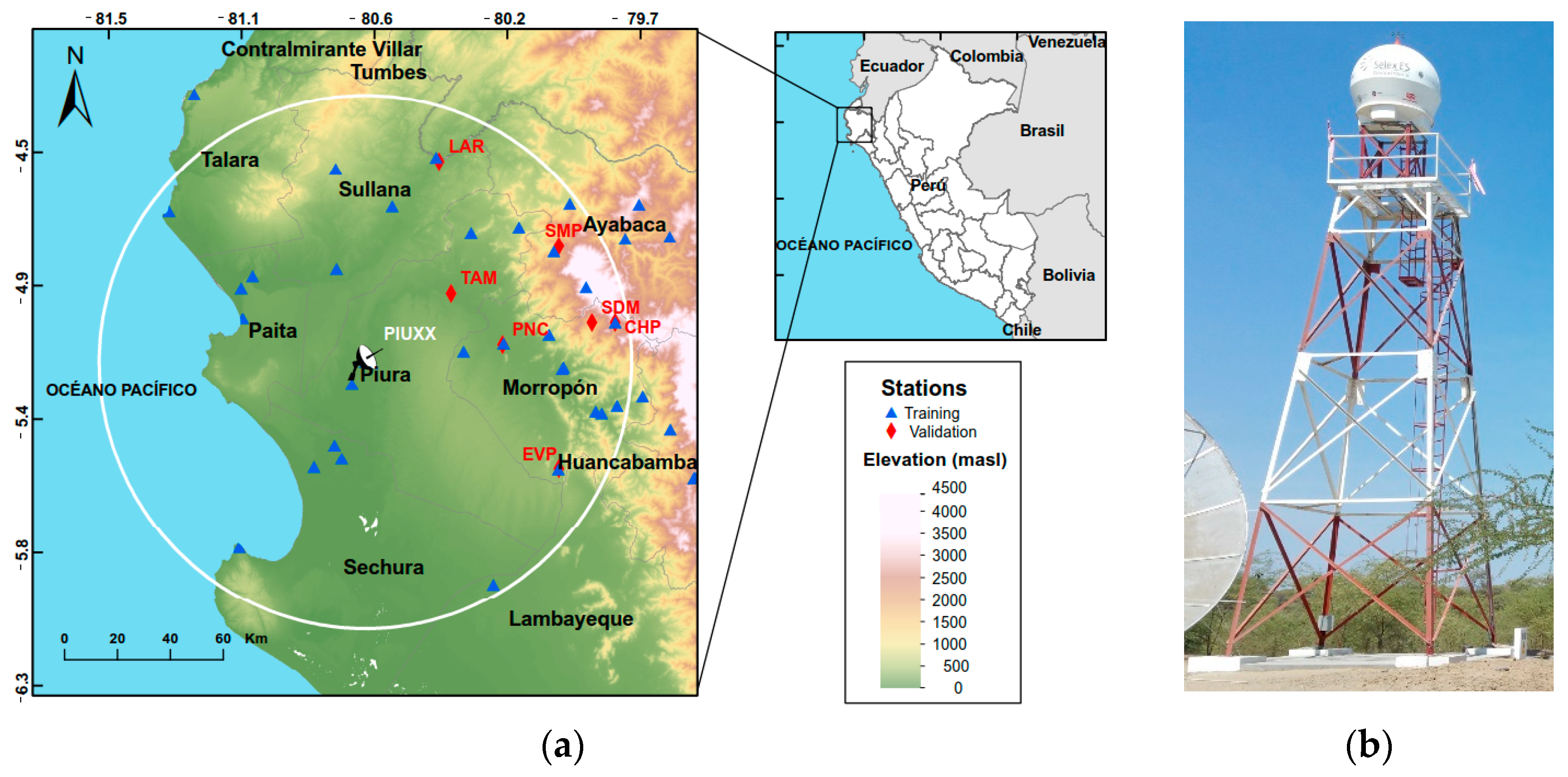
The radar system in Piura (PIUXX; Figure 1) was installed in May 2019 in the campus of the Universidad de Piura, and the first relevant data were captured with the onset of the 2019/2020 rainy season in October 2019. Technical characteristics are detailed in

Table 1. Technical specifications of RS 120 PIUXX.

Manufacturer	Country: Germany Brand: Selex (Now: LEONARDO) Model: RS120 Range: 100 km
Antenna	Diameter: 1.2 m Gain: 38.5 dB Side lobe elevation: −27 dBc Beam width (azimuth): 2° Beam width (elevation): 2° Rotation: 12 r.p.m. Azimuth tolerance: ±0.5°
Emitter	Peak power: 25 kW Frequency: 9410 (±30 MHz) Pulse repetition frequency (PRF): 833–1500 Hz Pulse duration: 500–1200 ns Pulse length (range resolution): 75–180 m
Receiver	Band width (1200 ns/500 ns): 3 MHz/7 MHz Minimum detectable signal: −100 dBm Dynamic range: 70 dB Noise figure: 6 dB
Signal processor	CPU: Intel Pentium Dual Core, Operating System: SuSe LINUX Radar A/D converter: 14 bit, 20 MS/s
Power supply	Radar: 100 VA/70 W Signal Processor: 100 VA/90 W Total system requirement incl. climatization and UPS: Max 500 VA

.

2.2. Radar Data Preprocessing

During 2019–2021, the radar system PIUXX has been in operation for 618 days, of which 302 days have provided valid reflectivity data and 195 days saw more than 1 mm of maximum rainfall. The radar supplies 5-min averages of reflectivity for 180 scan lines and 1000 range bins; thus the spatial resolution is 2° radial and about 100 m of distance (range gates). Each pixel value is averaged bit-wise from 60 scans, so in effect, the manufacturer applies averaging on dBZ values. Implications of this have been discussed in [36]. The raw data format (SELEX/Gematronik rainbow format) comprises an XML header with metadata and two highly compressed data BLOBs (binary large objects, zlib-compression) containing the reflectivity values transformed to 8-bit integers. Thus, the raw data are converted to dBZ by applying

$$dBZ=\frac{reflmin+raw\cdot \left(reflmax-reflmin\right)}{2^8}$$

(1)

where raw is the binary integer number and reflmin is −31.5 and reflmax is 95.5, giving the sensitivity range of the radar system in dBZ. Then, the dBZ data are stored with a polar coordinate system in netCDF format with 5-min resolution for further processing.

The polar data are submitted to preprocessing to address typical issues of raw radar data. The scheme presented here reduces the number of required preprocessing steps to obtain corrected reflectivities to just three basic calculations, which are (a) noise elimination, (b) clutter elimination, (c) integrated attenuation, and sensitivity correction using a limited set of empirical parameters.

First, unsystematic background noise is eliminated. For this, the complete 5-min time series of dBZ is converted to Z-values, and the frequency of positive Z-values is determined for each pixel. Pixels with a frequency of positive Z higher than 4% are flagged as noise. The noise value is determined as the median along the time axis for each pixel. The resulting noise map is subtracted from each time step.

Secondly, temporary clutter is detected by the Gabella-Clutter [19] filter included in ωradlib (wradlib.org). Clutter pixels are set to Z = 0, and the clutter mask is retained for later use in interpolating missing reflectivity values.

Based on the experience with the similar radars in Ecuador [4], a correction of overall geometric and atmospheric attenuation is necessary, although the radar operating software from the manufacturer already applies some (undocumented) attenuation correction. The additional correction is required due to the high attenuation of X-band microwaves and the decreasing sensitivity with distance.

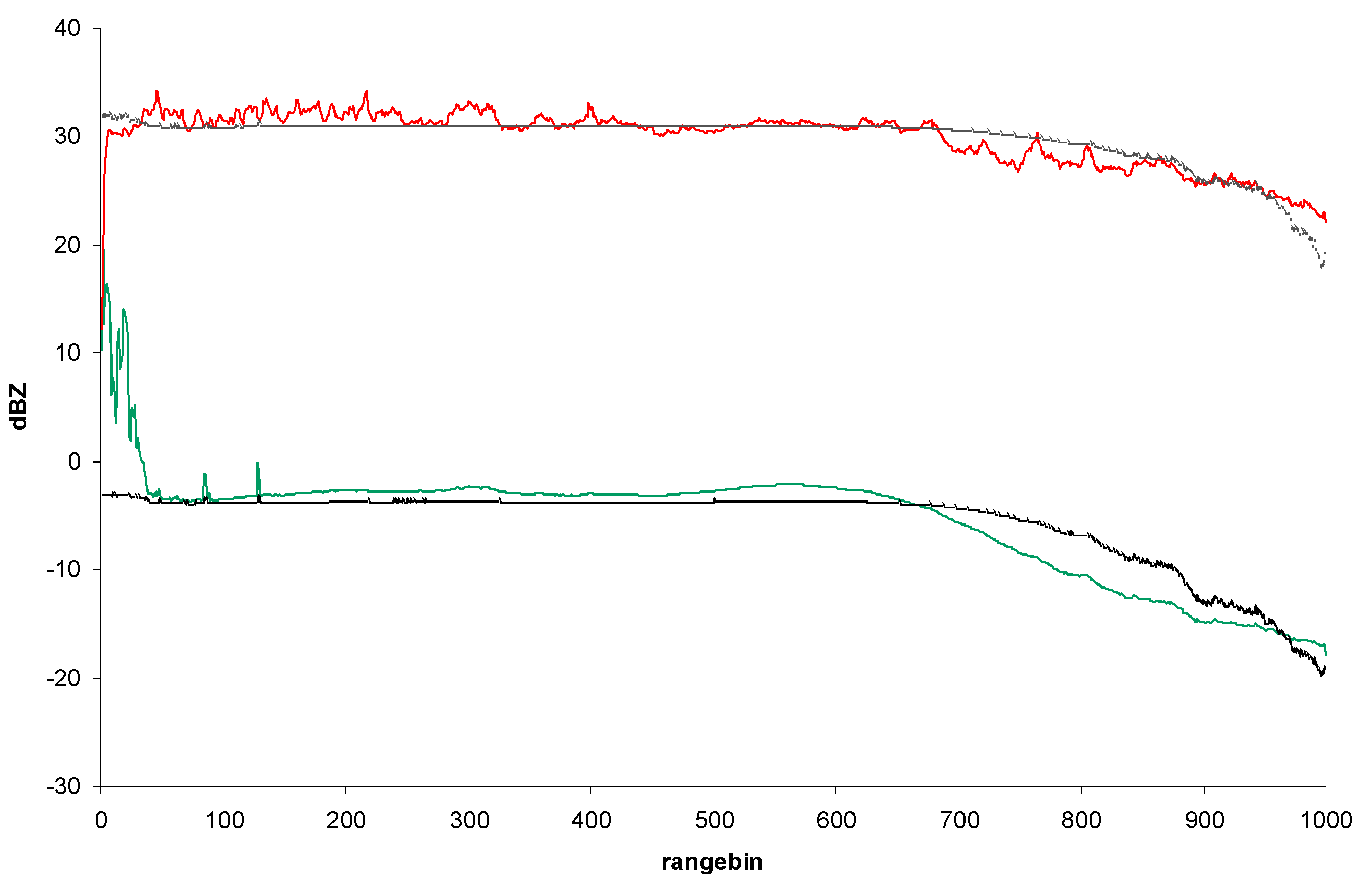
This leads to a loss of lower rain signals with distance and causes an increasing underestimation, particularly when aggregating temporally. The radial mean of all scan lines (Figure 2) results in a more or less straight line up to range-bin 600, so the attenuation starting at that distance from the radar becomes obvious. This correction method is discussed in detail in [21]. The required correction for the PIUXX radar was determined to be

$$Zc={10}^{\left(-2E6\cdot Z\right)+0.0043\cdot r}\mathrm{for}\mathrm{r}>600$$

(2)

where Z is the raw reflectivity, Zc is the corrected value, and r is the distance in range bins (not kilometers).

Finally, data gaps caused by the clutter and noise elimination steps are filled with the inpainting algorithm cv.INPAINT_TELEA as available from the Python library openCV (opencv.org). The location of such gaps is defined by the mask where Z = 0 due to clutter elimination.

Bright-band effects are rarely seen in the radar data because of the low elevation of the radar site and the sharp pencil beam (2° vertical) with a center elevation of 0°. The highest beam elevation of 3800 m at the full range (100 km) is almost always below the typical altitude of the melting layer as reported by [12] for the Andes.

Then, the resulting corrected radar data are transformed to Cartesian geographical coordinates and converted from UTC to local time to fit with the rain gauge data.

2.3. Rain Gauge Data

For calibration and validation (training and testing respectively in the random forest model), rain gauge data were collected from SENAMHI [41] (https://www.senamhi.gob.pe/?&p=estaciones accessed on 6 May 2021) and the climate stations were operated by Universidad de Piura (UDEP). In total, 53 rain gauge sites are available, but only 39 are inside the nominal range of the radar (100 km).

On average, 121 days of rainfall were registered at the 39 available calibration stations (

Table 2. Data sources and station types for rain gauges.

Station Type	n	Source
Conventional rain gauge (manual readout)	20	SENAMHI
Registering rain gauge (hourly data)	24	SENAMHI
Registering rain gauge (10-min data)	8	UDEP
Conventional rain gauge (manual readout)	1	UDEP

and Supplementary Materials; table of station metadata), with most of the rainy days occurring at the eastern margin of the domain, where humid climate prevails. Several stations in the Sechura desert only captured a few days of rainfall.

Initially, 13 stations were selected as validation sites (see map in Figure 1), but six of those had less than four days of rain data recorded, and so the list was reduced to seven stations.

To achieve the highest possible number of data points, the calibration scheme is based on daily aggregates of the available station data.

Data from SENAMHI are submitted to a quality check before being supplied, and uncertain values are eliminated from the time series. In addition, stations with a manual readout provide an estimation of very light rain marked as “T” in the time series. We have set those values to 0.01 mm of daily total. UDEP data are internally checked by procedures laid out in [42] considering the plausibility of temporal and spatial consistency of the whole dataset. The high temporal sampling of 10 min of several stations allows comparing rainfall measurements between neighboring stations along the time axis and also to other variables such as temperature, humidity, and radiation, indicating the probability for erroneous values.

2.4. Empirical Calibration Approach

To produce daily rainfall maps from rain gauge data, a larger domain around the radar circle was defined, covering 500 × 500 pixels, the inner 400 × 400 congruent with the bounding box of the radar domain. This avoids uncertainties at the margin, using stations beyond the radar range to support the interpolation. As the method of interpolation, universal kriging was selected due to its flexibility and capability to handle heterogeneously dispersed precipitation data [43]. The flexibility is warranted by using a variogram adapted to the observed data. We tested different variogram types such as exponential, spherical, and Gaussian, but the linear variogram type showed the best fit to the available data, although they include several data gaps due to operational breaks at different rain gauge sites. The interpolation result was validated against a set of seven of the 53 available rain gauge sites, aiming at the highest r² possible (Figure 3). The selection criteria for the validation sites were to have at least five days of gauge and reflectivity data while maintaining a large enough spatial coverage. Optimization runs found the best values for the linear variogram to be slope = 0.5 and nugget = 0.1 with the r² value between 0.42 and 0.91 for the different stations.

The central idea of the empirical calibration approach is to use the daily available station data to convert and adjust the radar reflectivity values to match the observed rainfall at the ground station. This represents a mean field bias correction in the sense of [44]. It leads to the rainfall distribution being derived from radar data, while the rainfall amount comes from the ground sites. It also differs from many other approaches published, which separate the reflectivity conversion and the bias correction. Here, those steps are integrated into the parameter setting for the Z–R relation. The Z–R relation consequently is now just a statistical approximation as [23] proposed.

Mathematically, the approach is based on the well-known empirical radar equation

$$Z=A\cdot R^b.$$

(3)

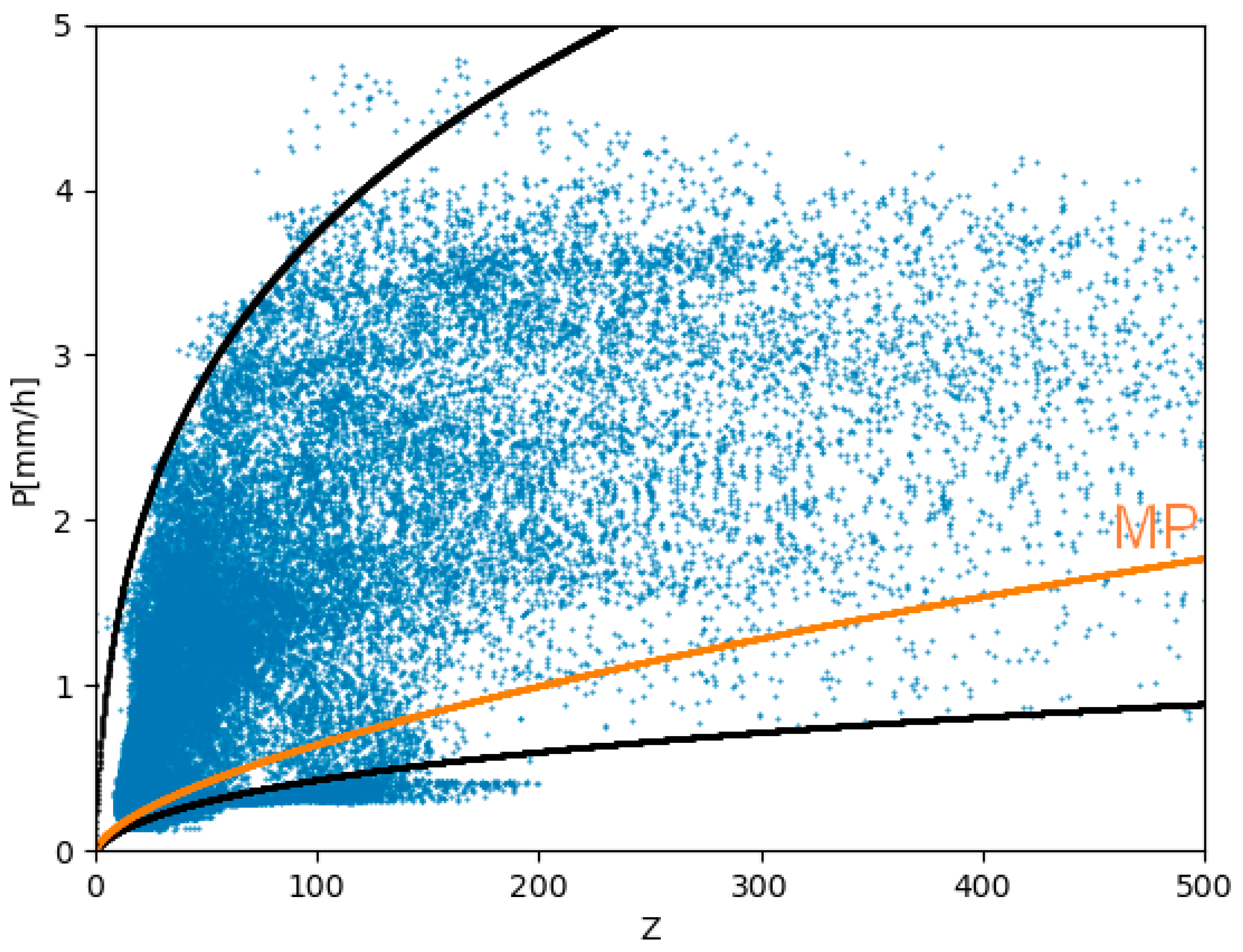
With the reflectivity Z, rain rate R, and the empirical parameters A and b, to reduce the problem to a linear equation, first, an approximate value for b is determined. From the overall mean of corrected radar Z values and the interpolated rain rate, a curvefit of the regression model (Z/A)^(1/b) is employed (Figure 4), resulting in a parameter set of A = 40 and b = 1.6 albeit with a very low coefficient of correlation, which is later addressed by modifying A and b to daily conditions. As rain gauge data are available as daily totals, the daily mean of Z is related to the daily rain total, although the averaging of Z may violate the equality of the Z–R-relation. As the internal software from the manufacturer already applies averaging on dBZ, the equality assumption can be discarded anyway [45]. So, a further transformation is required to linearize the final values for QPE. The median b0 of parameter b is used as a starting point for the daily calibration, and from iterative validation runs, a general empirical relation between b and Z at coordinates i,j is determined:

$${b^{\prime }}_{i,j}=b0+\frac{log\left(Z_{i,j}\right)}{2}$$

(4)

where b′_i,j is the reflectivity-dependent pixel-wise value for b. The constant 2 scales b′ to a range of 1.0 to 4.5 with a median of 1.6. Higher values of b′ are theoretically possible but will yield QPE values below the detection threshold of the radars (<0.08 mm per day). In effect, this is just a range compression for Z, which is required for highly sensitive X-band microwaves. Then, QPE values are calculated by using this variable exponent in the Z–R relation.

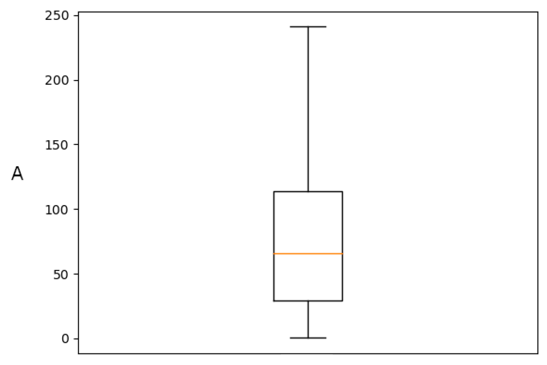
The A parameter is derived daily from each calibration station by inverting Equation (3) and using daily rainfall P:

$$A_{i,j}=\frac{Z_{i,j}}{P_{i,j}^{{b^{\prime }}_{i,j}}}$$

(5)

For P, a daily varying set of rain gauge sites is selected according to data availability and the positive rainfall value associated with non-zero reflectivity. Then, the resulting A values are interpolated to supply a value for each pixel of the radar domain, thus producing a daily matrix of spatially variable A. For days with less than three rain records, the A matrix of the previous day is used, assuming that atmospheric conditions remain stable. If no previous A matrix is available, the mean matrix from the annual means is used. Overall, these choices have little influence, because days with relevant rain always supply enough data for the calculation of a current A matrix.

The value range for A is shown in Figure 5, and the lowest RMSE for the comparison of mean Z vs. mean P is given at an A value of 40 with 0.608 mmh⁻¹.

The method integrates the mean field bias correction [44] and spatially variable field bias correction [27] into the basic radar equation, thus avoiding additional post-processing steps.

With the daily matrices of A, QPE is calculated as

$$QPE={Z^{\prime }}_{i,j}\cdot A_{i,j}$$

(6)

where Z′ is the transformed reflectivity Z^1/b′.

2.5. Machine Learning Approach: Random Forest

Random forest (RF) [37] is a machine learning (ML) technique from the decision tree-based family. It consists of several decision trees that are randomly and equally distributed. The final result is obtained from any aggregation of the individual results from each tree, the average in the most common case. Thus, this ML technique belongs to the ensemble methods. One of the main advantages of RF is the generation of the n datasets to build the n trees in the forest by using the bootstrapping method. Here, each dataset is generated from random samples with replacement of the original data. This ensures that a different dataset is used to build each decision tree and as a consequence adds robustness to the model. During the tree construction, the variable used in each node is selected from a group of randomly selected variables. The one that produces the lowest sum of square residuals is used to set the binary rule at the node. The iterative process continues until the tree reaches a defined depth. Since the subset of selected variables to build each tree is randomly chosen, this ensures low correlated trees. In addition, RF uses a third part of the data at every tree for internal validation (out-of-bag, OOB). This has the purpose of guaranteeing unbiased estimations of the error and also supports the calculation of the feature importance of the variables used to build the trees. Nevertheless, a major drawback of RF lies in the fact that the predicted value is the mean value from all tree predictions, and therefore, low values tend to be overestimated while higher values are underestimated.

For this study, we used the RF algorithm implemented in the Python library scikit-learn (version 0.21). The list and description of all hyperparameters defined in this algorithm is provided in

Table 3. Description of Rf hyperparameters defined in the implementation of the scikit-learn library (version 0.21).

Hyperparameter	Description	Default Value
criterion	Metric used to evaluate the quality of a split.	mean squared error
max_depth	Maximum depth of a tree.	‘none’ (until all leaves are pure)
max_features	Maximum number of random features to be used while building an individual tree.	total number of features
max_leaf_nodes	Maximum number of leaf nodes.	unlimited number of leaf nodes
max_samples	Maximum number of samples for training each tree.	all samples
min_samples_leaf	Minimum number of samples that belong to a leaf node.	1
min_samples_split	Minimum number of samples allowed to split an internal node.	2
n_estimators	The total number of trees in the forest.	100

.

The RF model was trained by using data of 558 daily samples from 27 training rain gauge stations where radar and rain gauge data were concurrent. From these, rain observations were obtained at a daily frequency and used as a target variable. The input features described in

Table 4. Features used in the random forest model for radar rainfall retrieval.

Feature Name	Description
Longitude	Longitude
Latitude	Latitude
Altitude	Altitude
Distance	Distance from radar
Avg Z temporal	5-min temporal average reflectivity (1-day window)
Std Z temporal	5-min temporal standard deviation reflectivity (1-day window)
Max Z temporal	5-min temporal maximum reflectivity (1-day window)
Sum Z temporal	5-min temporal accumulation of reflectivity (1-day window)
Avg u component temporal	5-min temporal average u component (1-day window)
Std u component temporal	5-min temporal standard deviation u component (1-day window)
Avg v component temporal	5-min temporal average v component (1-day window)
Std v component temporal	5-min temporal standard deviation v component (1-day window)
Avg Z temporal/Altitude	Quotient of 5-min temporal average reflectivity (1-day window) and altitude

were extracted from the 5-min radar images corresponding to those daily samples. Unlike their counterparts, RF works fairly well while using default hyperparameters values [40], and some studies mainly focus on the optimization of the number of trees (n_estimators) and number of features (max_features) [33]. Nonetheless, a recent study extensively evaluated the sensitivity of all RF hyperparameters in a runoff forecasting application by using radar data and found that the three hyperparameters that highly influenced the random forest regressor were the number of trees (n_estimators), the maximum number of features (max_features), and the maximum depth of a tree (max_depth) [46]. Therefore, in this study, we focused on the optimization of these three hyperparameters by using a grid search approach. Thus, a vector of possible values for each of these hyperparameters was defined and set for the grid search implementation (n_estimators = (100, 150, 200, 300, 400, 500, 600), max_features = (total number of features [13], square root of total number of features [4]), max_depth = (3, 5, 8, 10, 13, 15, 20)). Here, exhaustive combinations of all hyperparameters were used to build independent models (i.e., one set of hyperparameters defines one model) and to perform their evaluation (OOB score) by using a K-fold cross-validation. Thus, K-1 folds were used for training while the remaining fold was used for testing. This process is applied k iterations, and thus, each fold is used exactly once as the testing dataset. Finally, the intermediate results for evaluation (i.e., one per iteration) are averages, and therefore, a final estimation of the model performance is obtained.

An additional 104 samples were used for the testing phase; these correspond to 7 stations distributed on a horizontal line from the center of the radar to the east where the rainfall is more frequent and in a higher amount. It is worth mentioning that the testing phase is equivalent to the validation phase in the empirical approach (i.e., independent data, which has not been used before, is used to evaluate the performance of the model).

2.6. Input Features

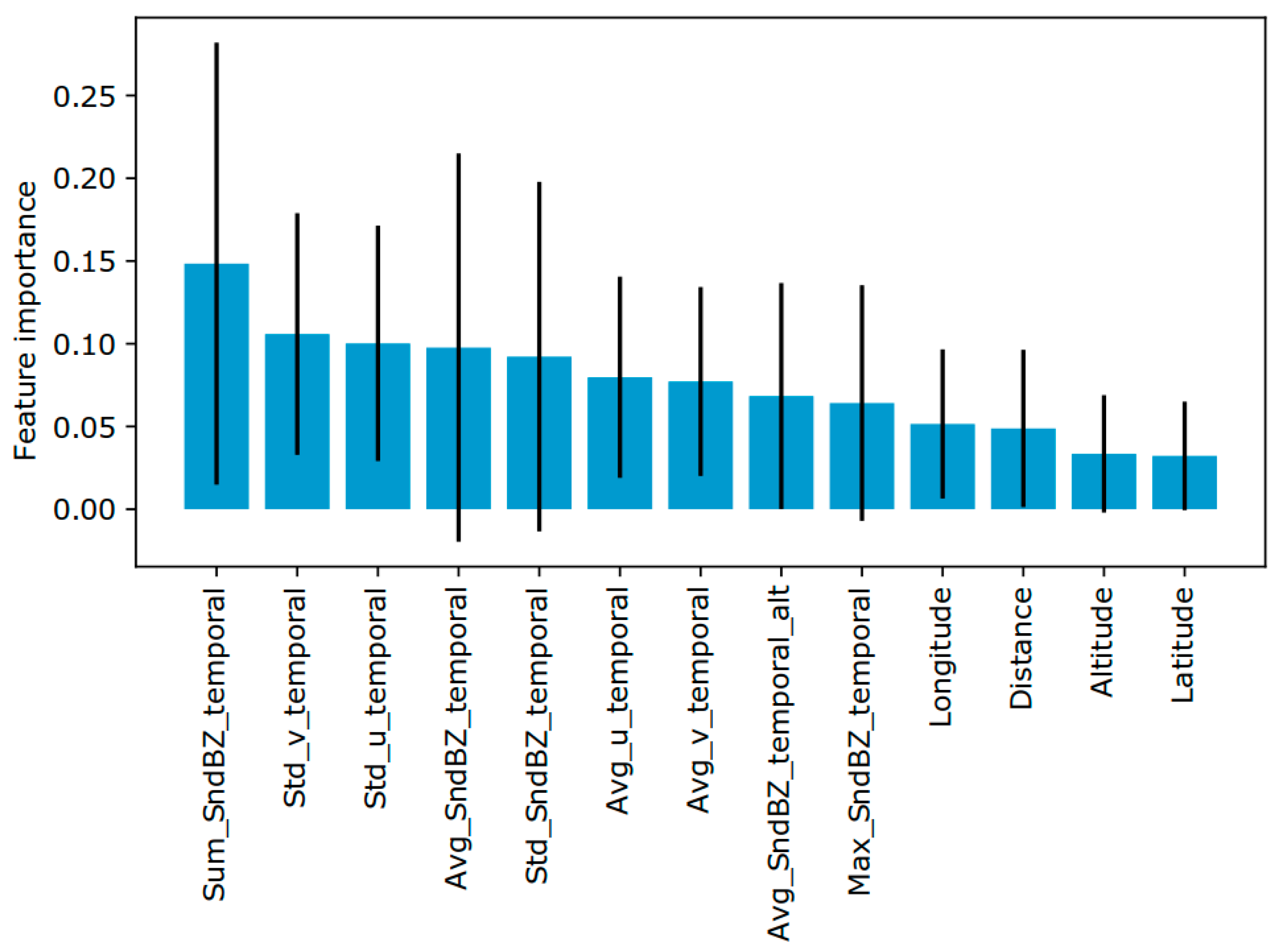
Following the concept of feature engineering in radar QPE derivation introduced by [30], several input features were derived to synthesize temporal characteristics occurring daily on the pixel of interest (e.g., average of reflectivity in a day by using 5-min radar observations). As a previous step, a median filter was applied to all radar images, which aims to compensate for common measurement errors due to altitude and wind. As an additional feature, the 5-min radar reflectivity images were analyzed to derive movement vectors of the rainstorms detected. For this, the whole time series was processed with the optical flow algorithm Dual-TVL1 [47] as available from the OpenCV computer vision library (OpenCV.org). The output is used in the form of the u (zonal) and v (meridional) vector in the feature set. Finally, more traditional predictors such as the coordinates, distance from the radar, and altitude were used. Table 4 shows the details for the interpretation of each feature used in the RF model.

Moreover, a feature importance analysis [40] was performed mainly to gather some insights in regard to the influence of the input features on the model but not for reducing the dimensionality of the problem, which is not necessary because the number of features is reduced. For this, each feature of the model was shuffled (i.e., breaking the relation of the feature and the output of the model) and then, the error model on the OOB sample (i.e., 33% of the training dataset) was evaluated by using the scikit-learn library of Python [48].

2.7. Statistical Metrics

To assess the quality of the parametrization, the main aim is to minimize deviations between radar QPE and rainfall observed at the validation sites. The data products used for this are the daily totals from (a) the radar QPE at the validation sites and (b) the daily validation rain gauge data along the whole time series of 618 days.

Furthermore, the overall detection rate for positive radar reflectivity is compared for the complete time series at the rain gauge sites, resulting in 24,102 data points (618 days at 39 sites), and error metrics for the whole dataset are calculated.

A full set of statistical error metrics is calculated with the wradlib-verify module where the aim is to balance high correlation measures with low error margins. Of these, the correlation coefficient, r², the Spearman rank correlation coefficient, root mean squared error (RMSE), mean absolute error (MAE), and percentage bias are chosen as diagnostic variables for the parameter optimization.

3. Results

The principal products of the preprocessing are daily fields of reflectivity rearranged to local time. This allows assessing the detection sensitivity for rainfall, and unsurprisingly, the radar data have a much higher detection rate, due to them being an integral measurement of a volume of the atmosphere, while rain gauges only sample a very small surface area.

The detection rate for rainfall shows that one-third of all rainfall events are only detected by the radar, while it misses only 9% of rainfall events measured by rain gauges (

Table 5. Comparison of detection rate for rainfall. Radar reflectivity is submitted to a 3 × 3 median filter to compensate for small errors in pixel location caused by the polar–Cartesian conversion.

	Radar > 0	Radar = 0
Rain gauge > 0	1383 (6%)	2134 (9%)
Rain gauge = 0	8103 (34%)	6702 (28%)

n = 24,102; missing data = 5780 (23%) 39 stations during 618 days.

), which is possibly due to the sectors with strong beam blockage and attenuation, which cannot be completely compensated.

These basic findings are supportive of both calibration approaches, which are evaluated in the following.

3.1. Validation of the Empirical Method

The main objective of the calibration effort is to minimize the scatter between observed daily rainfall at the validation sites and the calculated radar QPE. Figure 6 shows the result of the validation for the daily totals at the seven validation sites within the radar domain, using the best parameter set as detailed above. Validation data were selected with the objective to capture extreme events and to cover the strong zonal gradient; thus, the full dataset contains several sites in the dry southwest of the domain, where wrong reports of zero rain may be included. This affects the regression result (

Table 6. Error metrics of QPE vs. P_obs (validation data) for the empirical approach.

Metric	All Data	Validation Data
Correlation coefficient	0.78	0.82
r2 Coefficient of determination	0.61	0.67
Spearman rank correlation coefficient	0.77	0.69
Mean absolute error	5.75	7.25
Percent bias	34.4	−13.8

) with an r value of 0.82 vs. 0.78 for all data. In addition, a substantial underestimation of the rain gauge values by QPE can be deduced from the low slope value. In contrast, regarding the full detection scale, the peak value of daily rainfall of 127.6 mm, observed on 2 March 2021 in the rain gauge data, is exceeded by the 144.8 mm in radar QPE.

The error metrics support the findings of the validation scatter plots, with an acceptable RMSE of around 10 mm/day across all seven validation sites and a relatively small underestimation with a pbias of −13.8, a mean error of −2.3, and a ratio above 1. The mean absolute error and the Spearman coefficient are higher for the full dataset.

3.2. Results Machine Learning Approach

A random forest model was developed and adapted to estimate daily rainfall from 5-min radar images. The optimized hyperparameters for the model were found at 200 trees, 10 random features, and 10 levels of depth. Figure 7 illustrates the variability of the OOB scores by applying all hyperparameter combinations grouped by the number of trees. It can be seen that the definition of 200 trees shows the lowest variability, and after that, there are only slight changes. Thus, by using more the than 200 trees, the sensitivity of the model to the other hyperparameters increased.

The results of the feature importance and evaluation of the performance of the model on the testing dataset are described in the following. Figure 8 shows, as expected, that the cumulative reflectivity on a daily basis is the most important feature. Interestingly, the standard deviation of the v-wind component is closely followed by its counterpart of the u-wind component as features with high importance for the model similarly to the average and standard deviation of the reflectivity along the day. The importance of the other features slowly decreases, showing that they have a comparable influence on the model. The longitude feature has a higher importance than the latitude. This makes sense by considering the rainfall pattern in the study site with higher frequency and amount toward the east. Finally, similarly to other studies in the region [30,49], we confirm that the terrain altitude does not play a significant role (i.e., low feature importance) in QPE.

Figure 9 shows the correlation of observed and estimated hourly rainfall applying the QPE random forest model to the entire test dataset. It can be observed that in general, lower rain rates are overestimated, while higher rain rates are underestimated. This is a common effect of random forest regression models because the final prediction is the result of the average prediction of all trees in the forest. The calculated metrics for goodness-of-fit during the training and testing phases are shown in

Table 7. Error metrics of QPE vs. P_obs for the random forest approach.

Metric	Training Data	Test Data
Correlation coefficient	0.94	0.65
r2 Coefficient of determination	0.89	0.42
Spearman rank correlation coefficient	0.78	0.56
RMSE	5.01	12.87
Mean absolute error	3.28	9.01
Mean error	0.03	1.08
Percent bias	0.3	6.8

. The influence of the higher values of precipitation may affect the testing metric results due to its underestimation. In addition to the averaging effect in the random forest technique, the low number of samples for higher precipitation could negatively affect the capability of the model for generalization.

3.3. Precipitation Climatology and Case Studies

One of the largest advantages of radar data is its high resolution in time and space. For this reason, most studies use radar data mainly for event-based case studies and frequently only for limited spatial extents. The capability for longer-term climatological analyses is tested for the calibrated data from the two methods compared here by deriving a mean precipitation climatology representing the two rainy seasons captured during the operational time of PIUXX.

Obviously, this is not comparable to real climatological analyses, which require much more observation time, but it helps to assess the performance of the different methods. The interpolated station data (Figure 10a) show the typical smoothed features well known from many precipitation maps. In our case, the strong zonal gradient is apparent, but almost half of the domain is shown as completely rain-free, which is not a proper representation of the real data from the rain gauges, where there were several records of rainfall in the drier western part.

The calibrated radar data are more in line with personal observation, the general east–west gradient is well represented in the empirically calibrated data (Figure 10b), and the outreach of the 50 mm isohyets underline that there is indeed a relevant amount of rainfall west of the radar site. In addition, several smaller mountain ranges in the north and west show up as regions of higher annual rainfall, which is proven by the denser vegetation cover present in these hills.

The RF-calibrated map (Figure 10c) has much higher rainfall amounts for most of the domain; only in the high Andes mountains to the east, it seems to underestimate both the rain gauge measurements and the empirical calibration (Figure 10d). From this comparison, it can be deduced that the empirical calibration resembles the reference data more closely, while the RF calibration seems susceptible to disturbances by the remaining noise. Specifically, in the closest range from the radar site, circular noise speckles seem to be misinterpreted as rain.

A similar result is given by the time-series comparison of QPE versus R (Figure 11). Here, the spatially averaged daily rainfall for the whole radar domain is plotted. For the derivation of the RF-calibrated time series, a radar buffer of 8 km from the center was omitted because of the remaining noise close to the radar. Apparently, the RF method shows rather high values for lower rainfall amounts but misses the high peaks that frequently occurred in March of 2021. The threshold between over- and underestimations is seen at daily values of 12 to 15 mm. A detailed insight of peak values shows that the RF-method is limited to maximum daily rain totals of 55 mm, while the highest recorded rain gauge value was 127.6 mm. The same day, the empirical approach overestimated the highest value by showing almost 145 mm.

To assess the event-based performance of the calibration efforts, the most extreme three days were selected for a case study, showing the full coverage of the radar and larger areas with peak values well beyond 100 mm per day (Figure 12).

Both calibration methods have difficulties in the range beyond 80 to 90 km from the radar site, but they show much more details of spatial variation. Specifically, the images from the 2nd of March feature some extreme rainfall spots in the hills north of the radar, where the interpolated data just have a smooth transition to zero. As seen before, the RF-calibration has lower peak values but shows a larger extent of values around 20 mm per day. On the 10th of March (bottom row in Figure 12), the empirical calibration seems to miss a larger rainfall area to the northeast of the center, while other storm cells in the near range are not captured by the RF calibration.

In general, the empirical calibration more closely matches the distribution seen in the interpolated data, while the RF calibration is completely independent of these, including potential errors in the rain gauge data, which may remain even after quality control.

4. Discussion

The preprocessing for the X-band-radar in Piura is composed of standard methods combined with specific calculations derived from the long experience with radar processing for the similar instruments in Ecuador [4], where radar operation began in 2002. In contrast to the topographical conditions in Ecuador, the Piura radar has an almost unobstructed view and has supplied excellent results for the observation period. The two years of data show that the study region is more frequently hit by extreme precipitation events than is assumed from the arid appearance of the landscape.

The manufacturer of the radar system proposes the use of the standard Marshall–Palmer Z–R relation with A = 200 and b = 1.6, but the results are inconsistent even if complex post-processing is applied.

The empirical calibration approach presented here differs from previously proposed methods (e.g., [45,50,51]) by combining several post-processing steps into the parameter setting for the Z–R relation. A variable A parameter for the Z–R relation had previously been used successfully in the calibration methods applied in Ecuador [4,21,22]. The continuous adaptation of the b parameter is a new way of addressing the long-lasting discussion about the correct set of parameters for Z–R. Our additional correction given by Equation (4) serves the purpose of a range compression of the Z-values, which tend to give extreme values of QPE for higher reflectivities. The reason for this behavior is the high sensitivity of X-band radar, especially when sporadic bright-band effects are involved, which may be occurring in the higher mountain regions in the study area in some cases of hail-bearing thunderstorms. This is also the reason why the b parameter used here departs strongly from the values of b known from literature (e.g., [27,52]) and by this loses its physical meaning of an expression of the drop size distribution. Hence, it avoids the complex task of measuring or estimating drop-size distributions and their relation to atmospheric conditions [23]. This is especially relevant for calibration schemes, which are intended for operational use, as drop size observations are either relatively uncertain and almost never available in real time for larger areas.

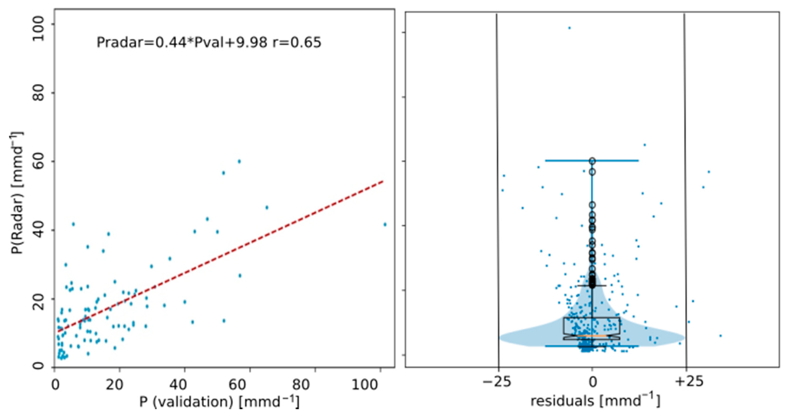
Although the empirical method shows a systematic under-estimation for lower daily rain rates (regression slope of 0.65), the full scale of stronger events is well captured, as is evidenced by the case study. The slight overestimation of the peak rainfall on 2 March 2021 (144 mm vs. 127 mm) may well be more realistic than the interpolated data, because it is quite unlikely that the rain gauges are always situated at the location of maximum rainfall. In addition, it has to be born in mind that the interpolated data already have a certain error margin and the spatial distribution of the validation sites is slightly biased due to the little rainfall in the southwestern sector of the radar domain. With the main purpose of capturing extreme events, this deficiency is considered as a minor problem, which will disappear when additional data come in. In addition, atmospheric and topographic conditions for the southwest sector of the domain are quite homogeneous, and thus, the Z–R relation derived at a few points can be reliably extrapolated to the less well-covered parts.

Improved results could be expected by using calibration data with higher temporal resolution, such as the half of available rain gauges with hourly samples. However, this was not done for two reasons: First, the coverage at the drier parts of the domain would be even less satisfying, with only five stations there reporting on an hourly basis. Second, the calibration schemes are developed as an operational tool for supplying near-real-time calibrated radar products. Due to the lag in reporting from the majority of the rain gauge sites, this can be achieved at best with daily data; higher rates of data transfer are currently not available. Another problem is the dislocation of radar detection vs. ground detection of rainfall due to wind and re-evaporation. For hourly data, there would be probably many more cases of missed rain events for either method, and the data availability would be impaired strongly.

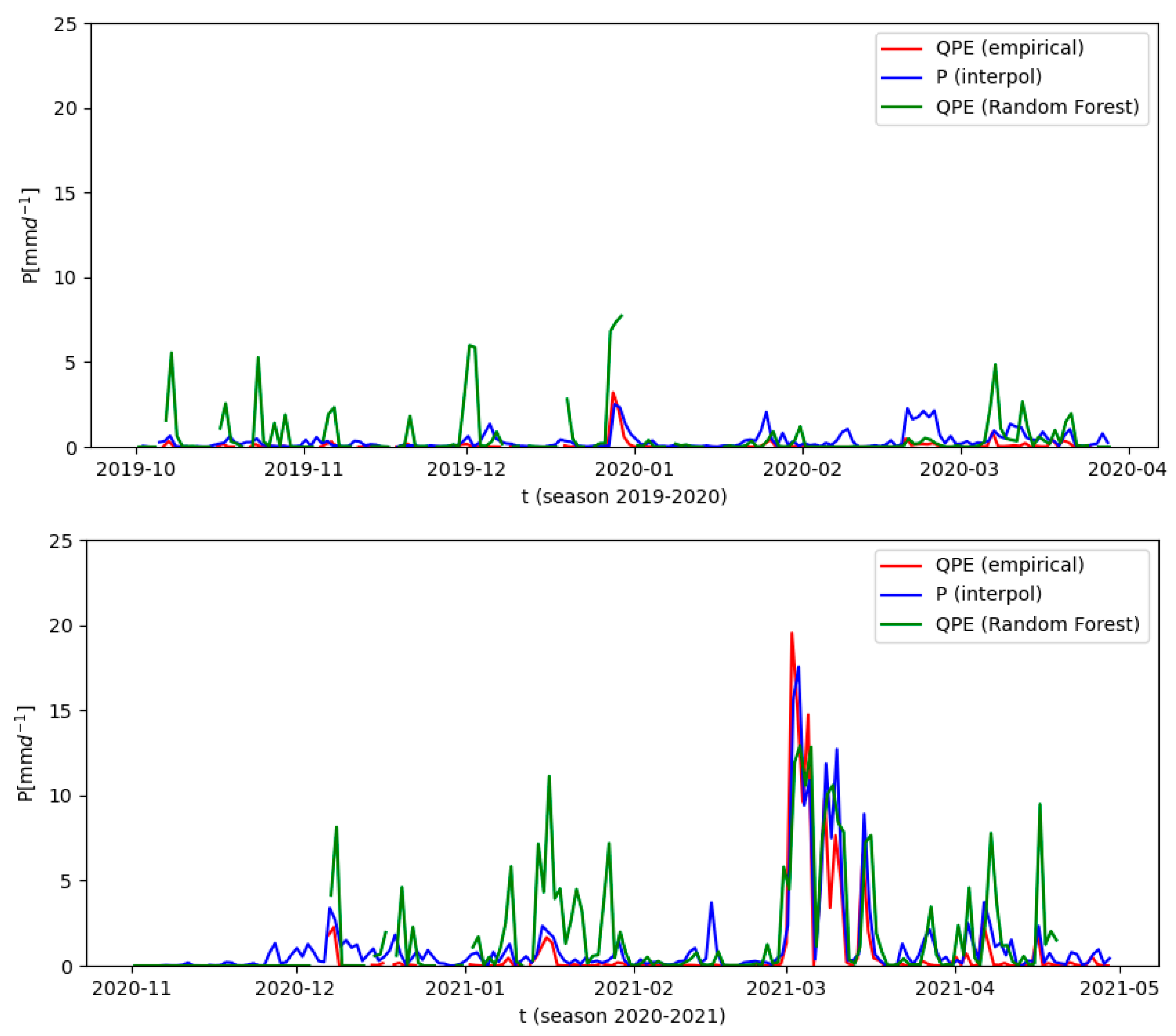
The RF calibration is quite superior in this aspect, as it does not depend on ancillary calibration values from rain gauges. When comparing the RF result to corrected reflectivity images, specifically the case studies, the approach is able to reproduce the spatial variability of rainfall in more detail and precision, although its quantitative performance is lower than its counterpart because of underestimation/overestimation of stronger rainfall. Limitations on the RF calibration scheme can be attributed to the reduced number of samples used for training the model in comparison with previous studies [30,31]. Particularly high precipitation records are scarce, and thus, the RF approach lacks enough training samples for generalization. In fact, there is only one data point available (127 mm on 2 March 2021), where an extreme value appears that is typical for the high variability in north Peru.

The results may indicate a slight overfitting because of the reduced number of samples for training and test. Although RF better handles reduced datasets, it would benefit from a higher number of predictors. Here, because of the high spatial resolution of radar data, the addition of other meteorological variables would need further treatment and evaluation before being used in the model. This might be interesting in the future along with a new evaluation of the RF model with a longer time series, and as a result, an increased number of rainfall events.

The biggest advantage is that the RF approach will benefit much more from additional training data obtainable in the near future, since machine learning-based models perform better when the training set increases. Additional extreme values will most likely improve on the underestimation of high rainfall values.

As with many other radar observations, there are specific but very localized problems with higher mountains. If there is more than 50% of beam obstruction, only few events of rainfall are captured, namely those where rainfall (also) occurs in higher atmospheric layers. While this is still useful for nowcasting and warning purposes, climatological analyses are not possible under those circumstances. Nevertheless, the good operational conditions in Piura will also help to improve the methodology for the Ecuador radars of the same type, because it is now possible to better separate the internal effects of the radar system from external effects caused by the topography. Furthermore, the RF approach bears quite some potential for being used for the whole radar network of all four instruments, although the amount of data and the potentially larger feature list will be computationally demanding.

For operational use, both approaches will be continued and validated on a frequent short-term basis. Possibly, a weighted mean of both approaches may give the best results and it may also be helpful to use additional upscaling factors, as suggested by the low slope values of the validation plots. This will also be monitored in the light of upcoming extreme events and their impact on environment, society, and infrastructure. Lastly, the primary application for the calibrated radar data is public use and support of authorities during extreme events.