
High-Performance VOC Quantification for IAQ Monitoring Using Advanced Sensor Systems and Deep Learning

 , , ,
, , ,  , , and
Abstract
:1. Introduction
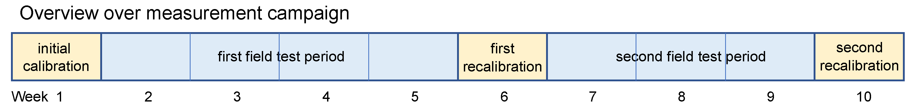
2. Materials and Methods
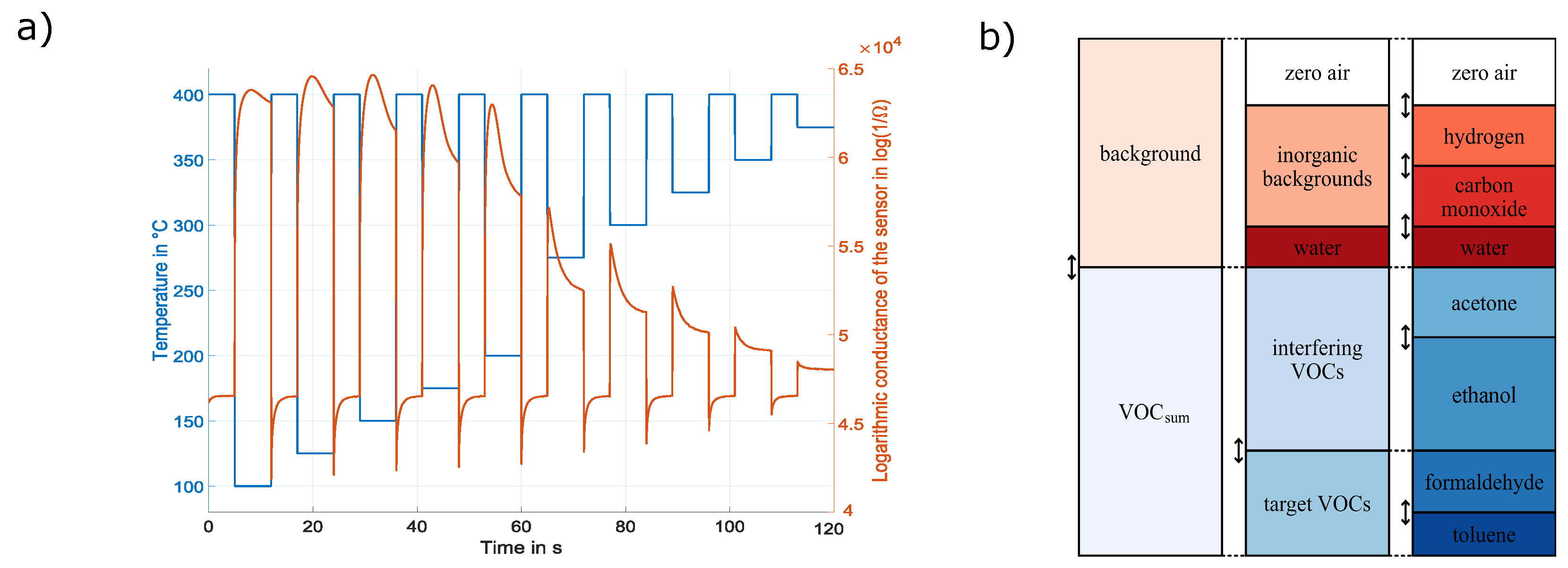
2.1. Dataset
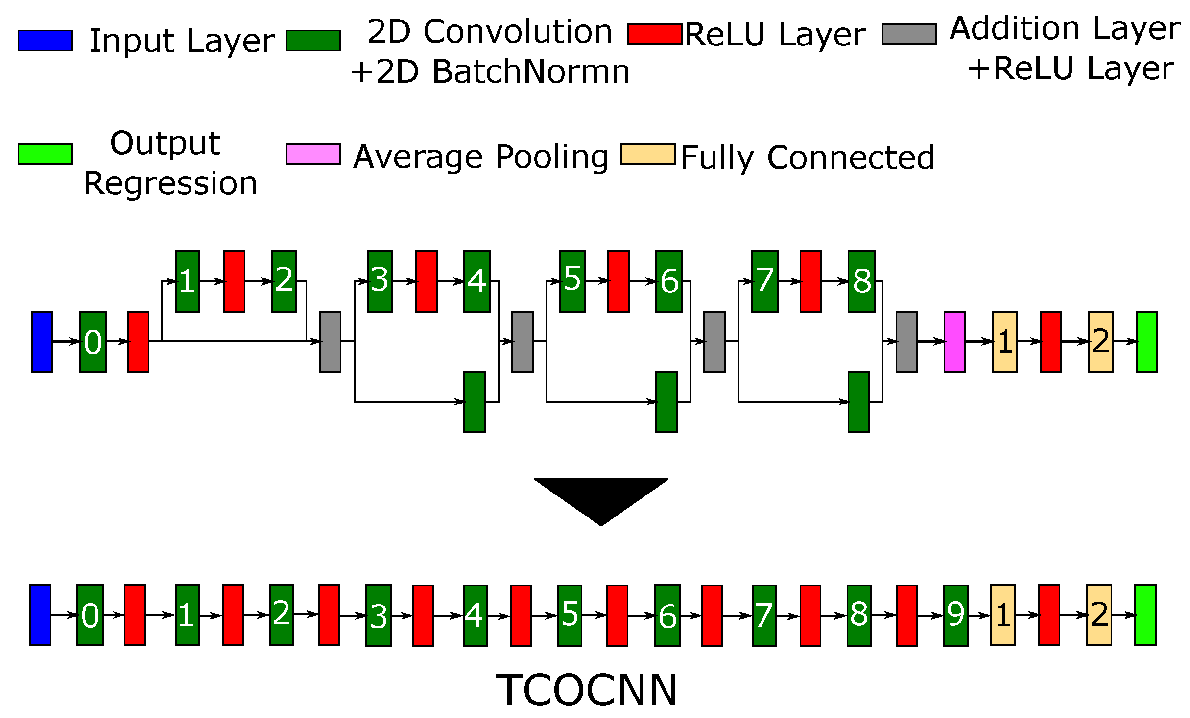
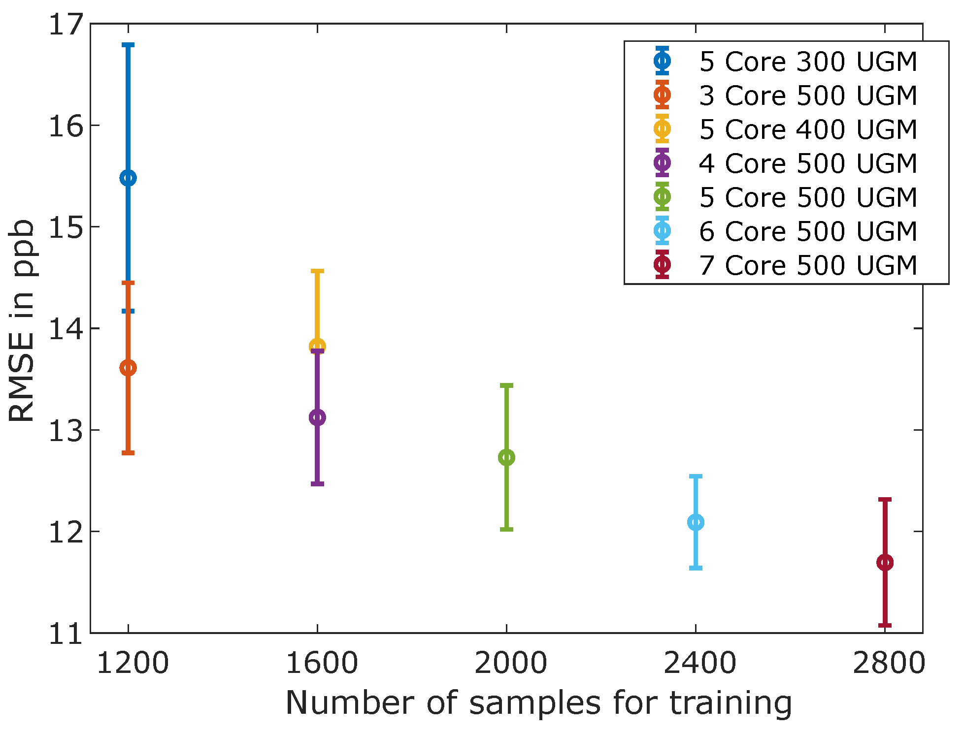
2.2. Model Building
2.3. Data Evaluation
3. Results
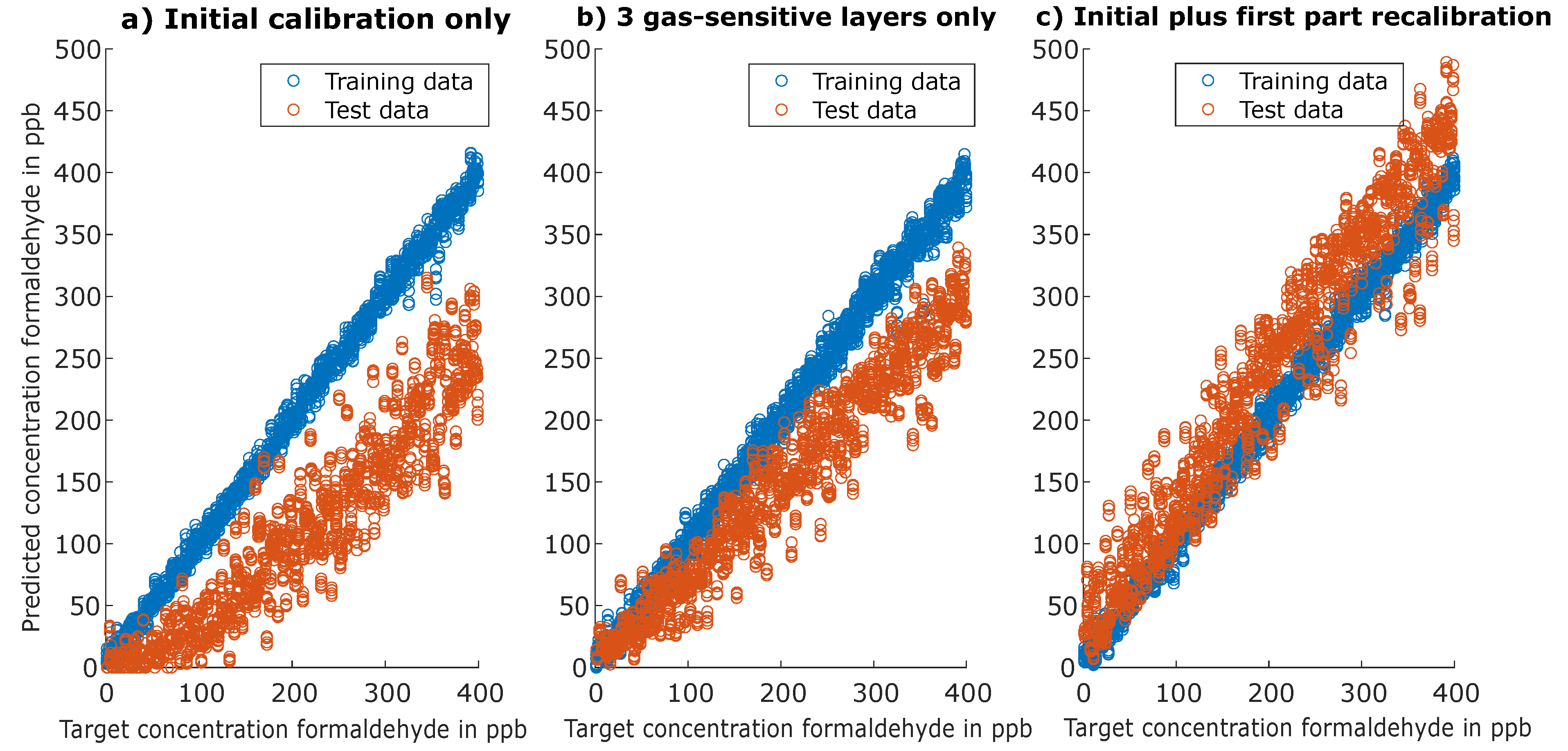
3.1. Calibration Results
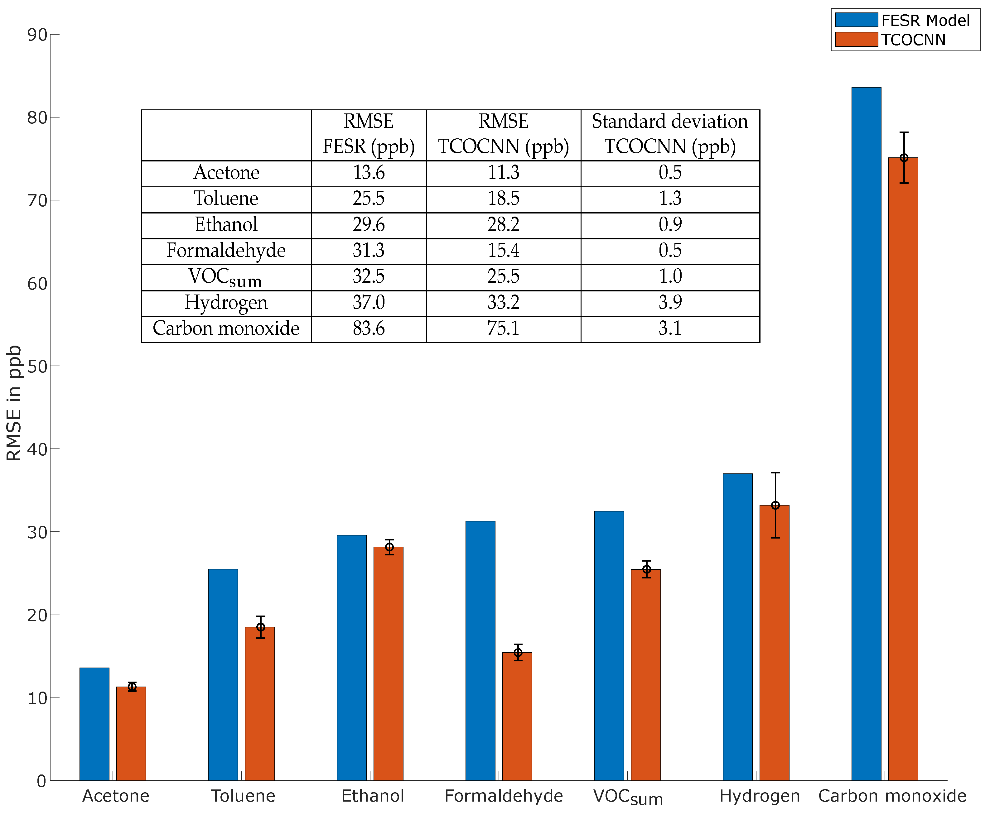
3.2. General Field Test Results
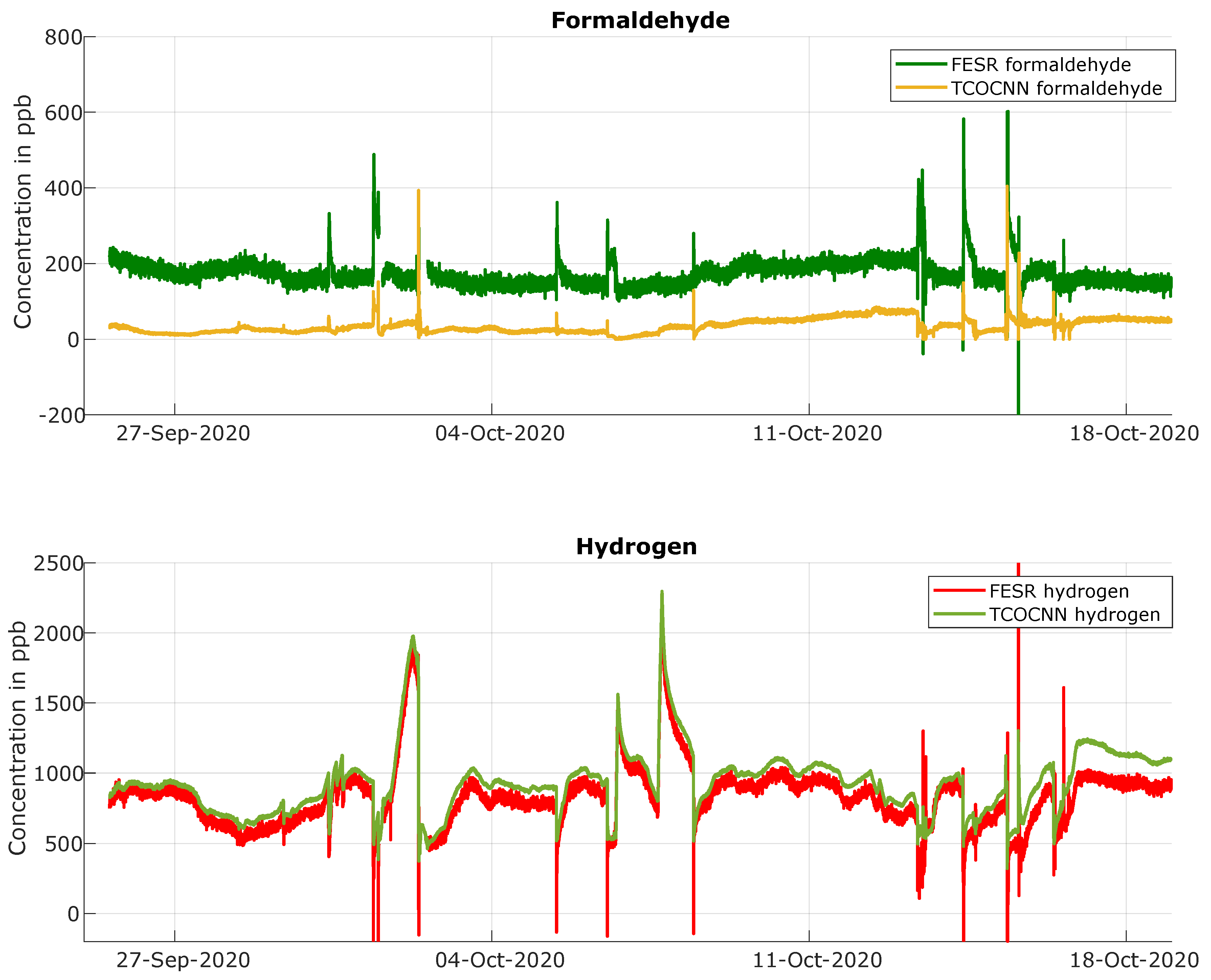
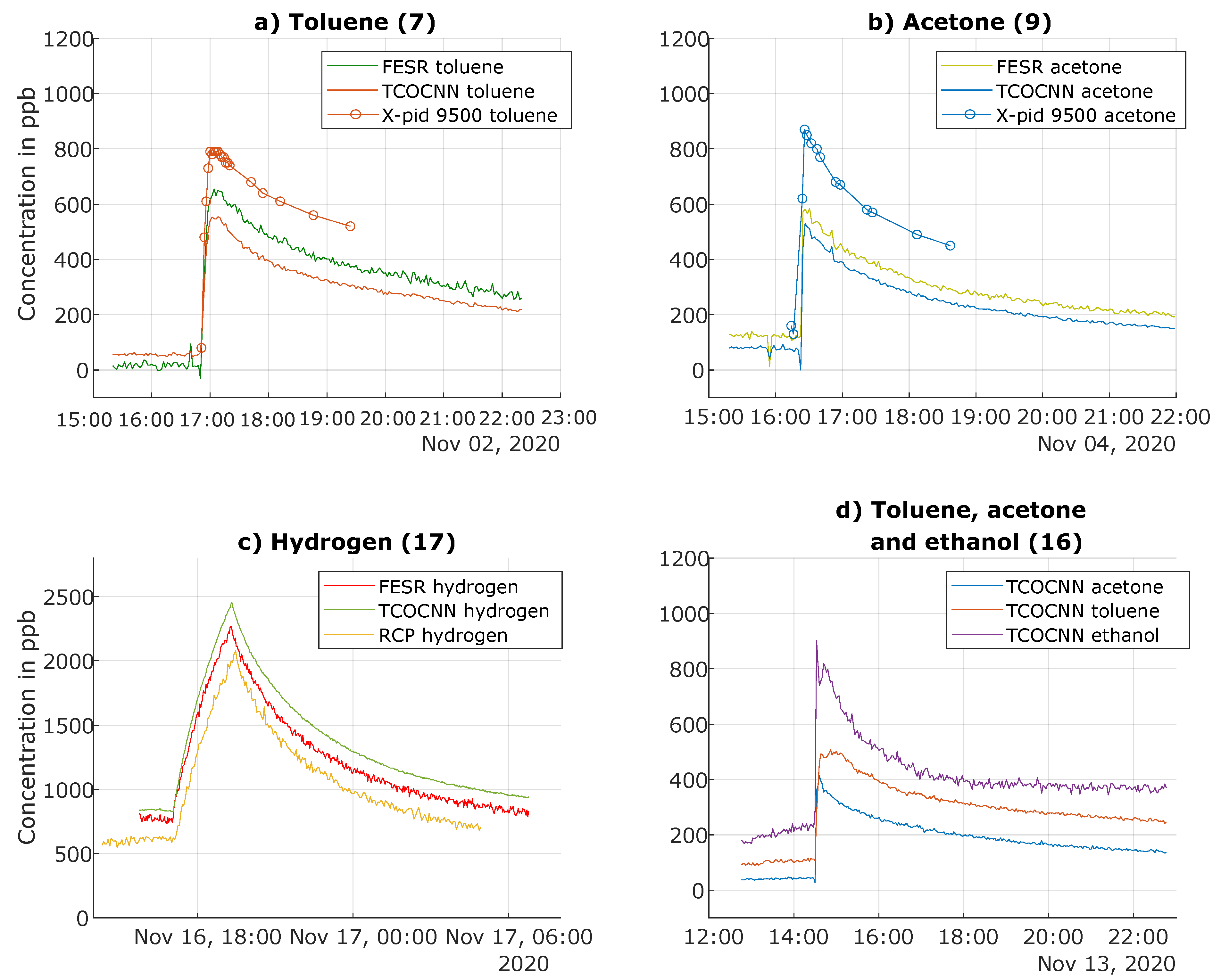
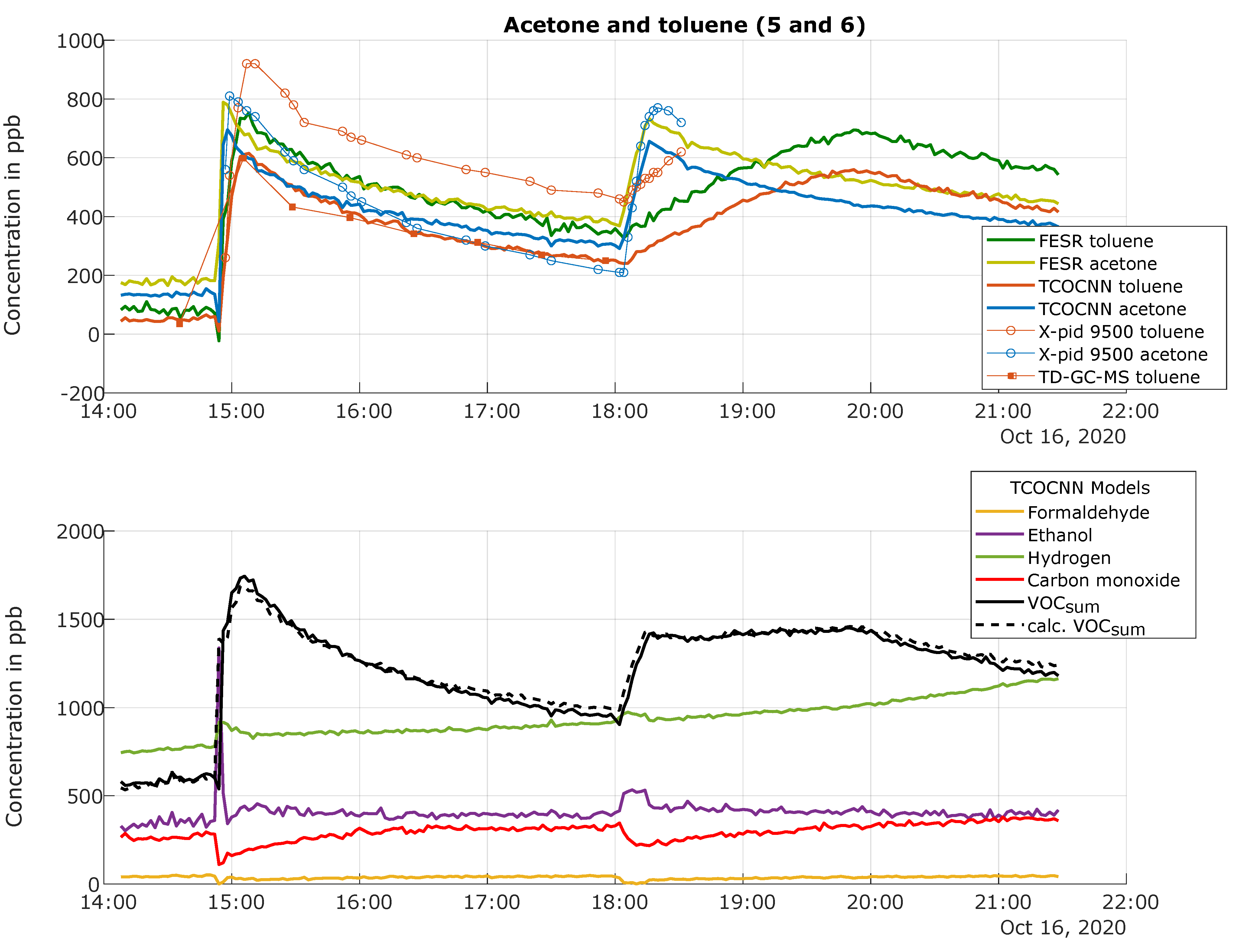
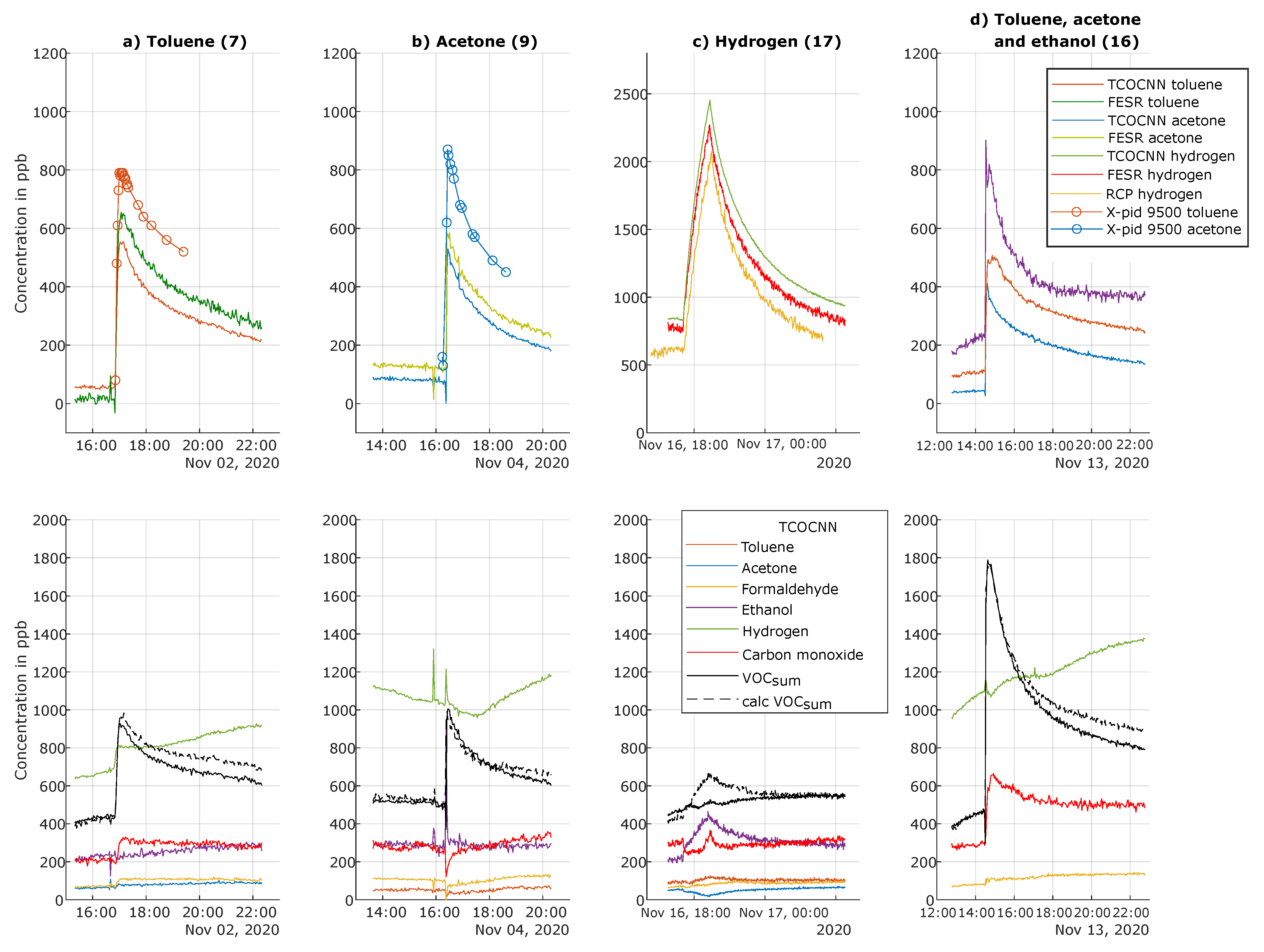
3.3. Results of the Release Tests for the Trained Gases
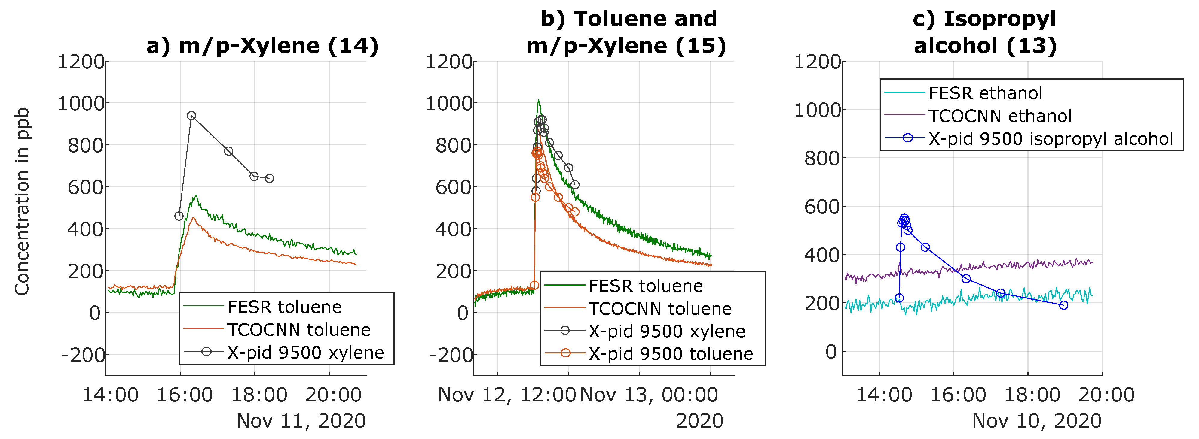
3.4. Results of Release Tests for Gases Not Trained
4. Discussion
5. Conclusions and Outlook
Author Contributions
Funding
Institutional Review Board Statement
Informed Consent Statement
Data Availability Statement
Acknowledgments
Conflicts of Interest
Abbreviations
| CNN | Convolutional neural network |
| FE | Feature extraction |
| FESR | Feature extraction selection regression |
| FS | Feature selection |
| GC-PID | Gas chromatograph with photo-ionization detection |
| GC-RCP | Gas chromatograph with reducing compound photometer |
| IAQ | Indoor air quality |
| LOQ | Limit of quantification |
| MFC | Mass flow controller |
| ML | Machine learning |
| MOS | Metal oxide semiconductor |
| NAS | Neural architecture search |
| PLSR | Partial least squares regression |
| PM | Particulate matter |
| RH | Relative humidity |
| RFE | Recursive feature elimination |
| RMSE | Root-mean-squared error |
| SVOC | Semivolatile organic compounds |
| TCO | Temperature-cycled operation |
| TD-GC-MS | Thermo-desorption gas chromatography mass spectrometry |
| UGM | Unique gas mixtures |
| VOC | Volatile organic compounds |
| VVOC | Very volatile organic compounds |
Appendix A


References
- Asikainen, A.; Carrer, P.; Kephalopoulos, S.; De Oliveira Fernandes, E.; Wargocki, P.; Hänninen, O. Reducing burden of disease from residential indoor air exposures in Europe (HEALTHVENT project). Environ. Health 2016, 15, 61–72. [Google Scholar] [CrossRef] [PubMed]
- Hauptmann, M.; Lubin, J.H.; Stewart, P.A.; Hayes, R.B.; Blair, A. Mortality from Solid Cancers among Workers in Formaldehyde Industries. Am. J. Epidemiol. 2004, 159, 1117–1130. [Google Scholar] [CrossRef] [PubMed] [Green Version]
- United Nations, Department of Economic and Social Affairs, Sustainable Development. Ensure Healthy Lives and Promote Well-Being for All at All Ages. Available online: https://sdgs.un.org/goals/goal3 (accessed on 15 October 2021).
- Valero, E. Advanced Nanomaterials for Inexpensive Gas Microsensors: Synthesis, Integration and Applications; Elsevier: Amsterdam, The Netherlands, 2020. [Google Scholar]
- Molhave, L.; Nielsen, G.D. Interpretation and Limitations of the Concept “Total Volatile Organic Compounds” (TVOC) as an Indicator of Human Responses to Exposures of Volatile Organic Compounds (VOC) in indoor air. Indoor Air 1992, 2, 65–77. [Google Scholar] [CrossRef]
- Salthammer, T. Very volatile organic compounds: An understudied class of indoor air pollutants. Indoor Air 2014, 26, 25–38. [Google Scholar] [CrossRef]
- Pettenkofer, M. Über den Luftwechsel in Wohngebäuden; Literarisch-Artistische Anstalt der J.G. Cotta’schen Buchhandlung: München, Germany, 1858. [Google Scholar]
- Yeoman, A.M.; Shaw, M.; Carslaw, N.; Murrells, T.; Passant, N.; Lewis, A.C. Simplified speciation and atmospheric volatile organic compound emission rates from non-aerosol personal care products. Indoor Air 2020, 30, 459–472. [Google Scholar] [CrossRef] [Green Version]
- Coggon, M.M.; McDonald, B.C.; Vlasenko, A.; Veres, P.R.; Bernard, F.; Koss, A.R.; Yuan, B.; Gilman, J.B.; Peischl, J.; Aikin, K.C.; et al. Diurnal Variability and Emission Pattern of Decamethylcyclopentasiloxane (D5) from the Application of Personal Care Products in Two North American Cities. Environ. Sci. Technol. 2018, 52, 5610–5618. [Google Scholar] [CrossRef]
- Mølhave, L. Indoor air pollution due to organic gases and vapours of solvents in building materials. Environ. Int. 1982, 8, 117–127. [Google Scholar] [CrossRef]
- Schütze, A.; Baur, T.; Leidinger, M.; Reimringer, W.; Jung, R.; Conrad, T.; Sauerwald, T. Highly Sensitive and Selective VOC Sensor Systems Based on Semiconductor Gas Sensors: How to? Environments 2017, 4, 20. [Google Scholar] [CrossRef] [Green Version]
- Haddad, S.; Synnefa, A.; Marcos, M.Á.P.; Paolini, R.; Delrue, S.; Prasad, D.; Santamouris, M. On the potential of demand-controlled ventilation system to enhance indoor air quality and thermal condition in Australian school classrooms. Energy Build. 2021, 238, 110838. [Google Scholar] [CrossRef]
- Baur, T.; Amann, J.; Schultealbert, C.; Schütze, A. Field Study of Metal Oxide Semiconductor Gas Sensors in Temperature Cycled Operation for Selective VOC Monitoring in Indoor Air. Atmosphere 2021, 12, 647. [Google Scholar] [CrossRef]
- Krizhevsky, A.; Sutskever, I.; Hinton, G.E. ImageNet Classification with Deep Convolutional Neural Networks. In Proceedings of the 25th International Conference on Neural Information Processing Systems, Lake Tahoe Nevada, CA, USA, 3–6 December 2012; Curran Associates Inc.: Red Hook, NY, USA, 2012; Volume 1, pp. 1097–1105. [Google Scholar]
- Gu, J.; Wang, Z.; Kuen, J.; Ma, L.; Shahroudy, A.; Shuai, B.; Liu, T.; Wang, X.; Wang, L.; Wang, G.; et al. Recent Advances in Convolutional Neural Networks. arXiv 2017, arXiv:1512.07108v6. [Google Scholar] [CrossRef] [Green Version]
- White, C.; Neiswanger, W.; Savani, Y. BANANAS: Bayesian Optimization with Neural Architectures for Neural Architecture Search. arXiv 2020, arXiv:1910.11858v3. [Google Scholar]
- Vito, S.D.; Massera, E.; Piga, M.; Martinotto, L.; Francia, G.D. On field calibration of an electronic nose for benzene estimation in an urban pollution monitoring scenario. Sens. Actuators B Chem. 2008, 129, 750–757. [Google Scholar] [CrossRef]
- Szczurek, A.; Szecówka, P.; Licznerski, B. Application of sensor array and neural networks for quantification of organic solvent vapours in air. Sens. Actuators B Chem. 1999, 58, 427–432. [Google Scholar] [CrossRef]
- Han, L.; Yu, C.; Xiao, K.; Zhao, X. A New Method of Mixed Gas Identification Based on a Convolutional Neural Network for Time Series Classification. Sensors 2019, 19, 1960. [Google Scholar] [CrossRef] [Green Version]
- Wang, S.; Hu, Y.; Burgues, J.; Marco, S.; Liu, S.C. Prediction of Gas Concentration Using Gated Recurrent Neural Networks. In Proceedings of the 2020 2nd IEEE International Conference on Artificial Intelligence Circuits and Systems (AICAS), Genova, Italy, 31 August–2 September 2020. [Google Scholar] [CrossRef]
- Chen, Z.; Zheng, Y.; Chen, K.; Li, H.; Jian, J. Concentration Estimator of Mixed VOC Gases Using Sensor Array With Neural Networks and Decision Tree Learning. IEEE Sens. J. 2017, 17, 1884–1892. [Google Scholar] [CrossRef]
- Xu, Y.; Meng, R.; Zhao, X. Research on a Gas Concentration Prediction Algorithm Based on Stacking. Sensors 2021, 21, 1597. [Google Scholar] [CrossRef]
- Benrekia, F.; Attari, M.; Bouhedda, M. Gas Sensors Characterization and Multilayer Perceptron (MLP) Hardware Implementation for Gas Identification Using a Field Programmable Gate Array (FPGA). Sensors 2013, 13, 2967–2985. [Google Scholar] [CrossRef]
- Feng, S.; Farha, F.; Li, Q.; Wan, Y.; Xu, Y.; Zhang, T.; Ning, H. Review on Smart Gas Sensing Technology. Sensors 2019, 19, 3760. [Google Scholar] [CrossRef] [Green Version]
- Bastuck, M. Improving the Performance of Gas Sensor Systems with Advanced Data Evaluation, Operation, and Calibration Methods. Ph.D. Thesis, Department Systems Engineering, Shaker Verlag, Saarland University, Düren, Germany, 2019. [Google Scholar]
- Rüffner, D.; Hoehne, F.; Bühler, J. New Digital Metal-Oxide (MOx) Sensor Platform. Sensors 2018, 18, 1052. [Google Scholar] [CrossRef] [Green Version]
- Baur, T.; Bastuck, M.; Schultealbert, C.; Sauerwald, T.; Schütze, A. Random gas mixtures for efficient gas sensor calibration. J. Sens. Sens. Syst. 2020, 9, 411–424. [Google Scholar] [CrossRef]
- Helwig, N.; Schüler, M.; Bur, C.; Schütze, A.; Sauerwald, T. Gas mixing apparatus for automated gas sensor characterization. Meas. Sci. Technol. 2014, 25, 055903. [Google Scholar] [CrossRef]
- Schultealbert, C.; Baur, T.; Schütze, A.; Sauerwald, T. Facile Quantification and Identification Techniques for Reducing Gases over a Wide Concentration Range Using a MOS Sensor in Temperature-Cycled Operation. Sensors 2018, 18, 744. [Google Scholar] [CrossRef] [PubMed] [Green Version]
- Baur, T.; Schütze, A.; Sauerwald, T. Optimierung des temperaturzyklischen Betriebs von Halbleitergassensoren (Optimization of temperature-cycled operation of semiconductor gas sensors). TM-Tech. Mess. 2015, 82, 187–195. [Google Scholar] [CrossRef]
- Schultealbert, C.; Baur, T.; Schütze, A.; Böttcher, S.; Sauerwald, T. A novel approach towards calibrated measurement of trace gases using metal oxide semiconductor sensors. Sens. Actuators B Chem. 2017, 239, 390–396. [Google Scholar] [CrossRef]
- Bastuck, M.; Baur, T.; Schütze, A. DAV³E a MATLAB toolbox for multivariate sensor data evaluation. J. Sens. Sens. Syst. 2018, 7, 489–506. [Google Scholar] [CrossRef] [Green Version]
- Robin, Y.; Goodarzi, P.; Baur, T.; Schultealbert, C.; Schütze, A.; Schneider, T. Machine Learning based calibration time reduction for Gas Sensors in Temperature Cycled Operation. In Proceedings of the 2021 IEEE International Instrumentation and Measurement Technology Conference (I2MTC), Glasgow, UK, 17–20 May 2021; pp. 1–6. [Google Scholar] [CrossRef]
- Snoek, J.; Larochelle, H.; Adams, R.P. Practical Bayesian Optimization of Machine Learning Algorithms. arXiv 2012, arXiv:1206.2944v2. [Google Scholar]
- Vergara, A.; Vembu, S.; Ayhan, T.; Ryan, M.A.; Homer, M.L.; Huerta, R. Chemical gas sensor drift compensation using classifier ensembles. Sens. Actuators B Chem. 2012, 166–167, 320–329. [Google Scholar] [CrossRef]
- Artursson, T.; Eklöv, T.; Lundström, I.; Martensson, P.; Sjöström, M.; Holmberg, M. Drift correction for gas sensors using multivariate methods. J. Chemom. 2000, 14, 711–723. [Google Scholar] [CrossRef]
- Amann, J.F. Möglichkeiten und Grenzen des Einsatzesvon Halbleitergassensoren im temperaturzyklischenBetrieb für die Messung der Innenraumluftqualität-Kalibrierung, Feldtest, Validierung. Master’s Thesis, Universität des Saarlandes, Saarbrücken, Germany, 2021. [Google Scholar]
- Bur, C.; Engel, M.; Horras, S.; Schütze, A. Drift compensation of virtual multisensor systems based on extended calibration. In Proceedings of the IMCS2014—The 15th International Meeting on Chemical Sensors (Poster Presentation), Buenos Aires, Argentina, 16–19 March 2014. [Google Scholar]
- Schleyer, E.B.R.; Wallasch, M. Das Luftmessnetz des Umweltbundesamtes; Umweltbundesamt: Dessau-Roßlau, Germany, 2013. [Google Scholar]
- WHO. WHO Regional Office for Europe Centers of Disease Control, WHO Guidelines for Indoor Air Quality: Selected Pollutants; World Health Organization: Copenhagen, Denmark, 2010; Volume 9, ISBN 978-92-890-0213-4. [Google Scholar]
- Schultealbert, C.; Amann, J.; Baur, T.; Schütze, A. Measuring Hydrogen in Indoor Air with a Selective Metal Oxide Semiconductor Sensor. Atmosphere 2021, 12, 366. [Google Scholar] [CrossRef]
- Schutze, A.; Gramm, A.; Ruhl, T. Identification of Organic Solvents by a Virtual Multisensor System With Hierarchical Classification. IEEE Sens. J. 2004, 4, 857–863. [Google Scholar] [CrossRef]


| Substance | Min. | Max. | Extended |
|---|---|---|---|
| Carbon monoxide | 150 ppb | 2000 ppb | - |
| Hydrogen | 400 ppb | 2000 ppb | 4000 ppb |
| Humidity | 25% RH | 70% RH | - |
| Acetone | 14 ppb | 300 ppb | 1000 ppb |
| Toluene | 4 ppb | 300 ppb | 1000 ppb |
| Formaldehyde | 1 ppb | 400 ppb | - |
| Ethanol | 4 ppb | 300 ppb | 1000 ppb |
| VOCsum | 300 ppb | 1200 ppb | - |
| Release | Time | Substance (Type of Release) | Released Amount of Substance (Approx. Increase in Room Conc.) |
|---|---|---|---|
| 5 | 16 October, 14:50 | Acetone (evaporation) Toluene (evaporation) | ∼600 ppb ∼600 ppb |
| 6 | 16 October, 18:00 | Acetone (evaporation) Toluene (evaporation) | ∼600 ppb ∼600 ppb |
| 7 | 2 November, 16:50 | Toluene (evaporation) | ∼600 ppb |
| 9 | 4 November, 16:22 | Acetone (evaporation) | ∼600 ppb |
| 13 | 10 November, 14:30 | Isopropyl alcohol (evaporation) | ∼600 ppb |
| 14 | 11 November, 15:49 | m/p-Xylene (evaporation) | ∼600 ppb |
| 15 | 12 November, 15:08 | Toluene (evaporation) m/p-Xylene (evaporation) | ∼600 ppb ∼600 ppb |
| 16 | 13 November, 14:30 | Acetone (evaporation) Toluene (evaporation) Ethanol (evaporation) | ∼600 ppb ∼600 ppb ∼664 ppb |
| 17 | 16 November, 17:06 | Hydrogen (MFC, gas cylinder) | 2000 ppb |
| Initial Learning Rate (Log Scale) | Number of Filters (First Two Layers) | Kernel Size (First Two Layers) | Stride Size (First Layer) | Dropout | Number of Neurons (FC) |
|---|---|---|---|---|---|
| 1 –9 | 60–240 | 40–80 | 15–45 | 30–50% | 1000–2500 |
| Parameter | Value |
|---|---|
| L2-regularization | 0.0001 |
| Stride size, even layer | 1 × 2 |
| Kernel size, other layer | 1 × 2 |
| Learn rate drop rate | 0.9 |
| Mini-batch size | 50 |
| Stride size, odd layer | 1 × 1 |
| Epochs | 75 |
| Learn rate drop period | 2 |
| Chemical Class (Representative) | P90 in g/m (ppb) | P95 in g/m (ppb) |
|---|---|---|
| Alcohols (ethanol) | 320 (∼170) | 520 (∼280) |
| Aldehydes (formaldehyde) | 340 (∼270) | 480 (∼390) |
| Aromatics (toluene) | 190 (∼50) | 370 (∼90) |
| Ketones (acetone) | 250 (∼100) | 420 (∼170) |
| Substance | Initial Learning Rate (Log Scale) | Number of Filters (First Two Layers) | Kernel Size (First Two Layers) | Stride Size (First Layer) | Dropout | Number of Neurons (FC) |
|---|---|---|---|---|---|---|
| Acetone | 1 | 142 | 48 | 34 | 31.65% | 1084 |
| Toluene | 2 | 240 | 69 | 17 | 37.06% | 2462 |
| Formaldehyde | 3 | 183 | 55 | 18 | 49.75% | 1188 |
| Ethanol | 2 | 228 | 73 | 34 | 49.55% | 2310 |
| VOCsum | 1 | 77 | 78 | 44 | 30.89% | 1373 |
| CO | 6 | 151 | 52 | 30 | 34.96% | 2468 |
| Hydrogen | 1 | 77 | 41 | 19 | 49.07% | 1088 |
| Standard Deviation FESR (ppb) | Standard Deviation TCOCNN (ppb) | |
|---|---|---|
| Toluene | 9.7 | 2.0 |
| Formaldehyde | 9.9 | 1.6 |
| Carbon monoxide | 33.6 | 5.5 |
| VOCsum | 15.8 | 4.5 |
| Acetone | 5.7 | 2.6 |
| Ethanol | 15.0 | 10.7 |
| Hydrogen | 19.0 | 3.7 |
Publisher’s Note: MDPI stays neutral with regard to jurisdictional claims in published maps and institutional affiliations. |
© 2021 by the authors. Licensee MDPI, Basel, Switzerland. This article is an open access article distributed under the terms and conditions of the Creative Commons Attribution (CC BY) license (https://creativecommons.org/licenses/by/4.0/).
Share and Cite
Robin, Y.; Amann, J.; Baur, T.; Goodarzi, P.; Schultealbert, C.; Schneider, T.; Schütze, A. High-Performance VOC Quantification for IAQ Monitoring Using Advanced Sensor Systems and Deep Learning. Atmosphere 2021, 12, 1487. https://doi.org/10.3390/atmos12111487
Robin Y, Amann J, Baur T, Goodarzi P, Schultealbert C, Schneider T, Schütze A. High-Performance VOC Quantification for IAQ Monitoring Using Advanced Sensor Systems and Deep Learning. Atmosphere. 2021; 12(11):1487. https://doi.org/10.3390/atmos12111487
Chicago/Turabian StyleRobin, Yannick, Johannes Amann, Tobias Baur, Payman Goodarzi, Caroline Schultealbert, Tizian Schneider, and Andreas Schütze. 2021. "High-Performance VOC Quantification for IAQ Monitoring Using Advanced Sensor Systems and Deep Learning" Atmosphere 12, no. 11: 1487. https://doi.org/10.3390/atmos12111487
APA StyleRobin, Y., Amann, J., Baur, T., Goodarzi, P., Schultealbert, C., Schneider, T., & Schütze, A. (2021). High-Performance VOC Quantification for IAQ Monitoring Using Advanced Sensor Systems and Deep Learning. Atmosphere, 12(11), 1487. https://doi.org/10.3390/atmos12111487