Tropospheric Refractivity Profile Estimation by GNSS Measurement at China Big-Triangle Points

Abstract

Atmospheric radio refractivity has an obvious influence on the signal transmission path and communication group delay effect. The uncertainty of water vapor distribution is the main reason for the large error of tropospheric refractive index modeling. According to the distribution and characteristics of water vapor pressure, temperature, and pressure, which are the basic components of the refractive index, a method for retrieving atmospheric refractivity profile based on GNSS (Global Navigation Satellite System) and meteorological sensor measurement is introduced and investigated in this study. The variation of the correlation between zenith wet delay and water vapor pressure is investigated and analyzed in detail. The partial pressure profiles of water vapor are retrieved with relevance vector machine method based on tropospheric zenith wet delay calculated by single ground-based GPS (Global Positioning System) receiver. The atmospheric temperature and pressure is calculated with the least square method, which is used to fit the coefficients of the polynomial model based on a large number of historical meteorological radiosonde data of local stations. By combining the water vapor pressure profile retrieving from single ground-based GPS and temperature and pressure profile from reference model, the refractivity profile can be obtained, which is compared to radiosonde measurements. The comparison results show that results of the proposed method are consistent with the results of radiosonde. By using over ten years’ (through 2008 to 2017) historical radiosonde meteorological data of different months at China Big-Triangle Points, i.e., Qingdao, Sanya, Kashi, and Jiamusi radiosonde stations, tropospheric radio refractivity profiles are retrieved and modeled. The comparison results present that the accuracies of refractivity profile of the proposed method at Qingdao, Sanya, Kashi, and Jiamusi are about 5.48, 5.63, 3.58, and 3.78 N-unit, respectively, and the annual average relative RMSE of refractivity at these stations are about 1.66, 1.53, 1.49, and 1.23%, respectively.

1. Introduction

It is well-known that refraction and time delay occur when electromagnetic wave propagates in the atmosphere as the changing properties of the atmosphere, the speed of propagation is altered, and the propagation path is also changed, which lead to a refraction error that severely disrupts the accuracy of radar detection, space tracking, satellite surveying and mapping, navigation, etc. The tasks of determining the profiles of the tropospheric refractive index and its characteristics are relevant for the both optical and radio ranges [1,2,3,4]. Tropospheric refractivity is a key parameter to evaluate the refraction error. As its variation in height is much greater than the horizontal direction, the accounting of atmospheric refractivity with different height is required so as to improve target tracking and navigation accuracy [5,6,7,8]. For this reason, some different atmospheric profile models were investigated based on a large number of data and theory. For example, Hopfield model [9] and segmented model [10], now as relatively accurate atmospheric prediction models, were developed by the atmospheric statics equation and ground meteorological data. While the actual atmosphere is not the same as the statics equation, the wet refractivity of those models lacks theoretical basis, and as a result, the results of the predicted models have a significant error with the actual atmosphere. Water vapor is a passive admixture and its dynamics depend on air temperature and wind speed fields, although water vapor is a small proportion in the whole atmosphere and has drastic changes with space and time, which makes it harder to monitor its distribution accurately [11,12,13].

There are also other methods to obtain atmospheric profile, such as radiosonde, Global Navigation Satellite System Meteorology (GNSS-MET), and water vapor radiometer. Radiosonde and water vapor radiometer are seen as high precision methods, while they suffer a higher cost and a lower temporal and spatial resolution. GNSS-MET is a potential method that has less cost than radiosonde, but higher precision than a traditional empirical model, moreover, it can be used in real time and has higher temporal and spatial resolution [14,15,16,17,18,19].

For ground-based GNSS remote sensing of the tropospheric refractivity profile, forward modeling is a process of calculating the refractivity profile based on the ray tracing algorithm, while inversion is a process of retrieving the refractivity profile by suitable algorithm based on tropospheric delay obtained by GNSS solution. Those inversion algorithms can be divided into two categories: one is to establish a distribution model of atmospheric parameters as a function of altitude, then solve model parameters using polynomial fitting, which is suitable for those atmospheric parameters changes regularly in profile distribution. The other is to build linear or non-linear regression statistics models of atmospheric parameters using a large amount of historical data, which is suitable for those atmospheric parameter changes in a random way and amplitude of fluctuations is more complicated and intense.

In this investigation, firstly, we retrieved the profile of water vapor pressure by non-linear regression statistics models using GPS measurement based on Relevance Vector Machine [20]. Secondly, atmospheric temperature profile was calculated based on least square curve fitting principle. Thirdly, atmospheric pressure profile was computed according to the gradient of temperature profile. At last, atmospheric refractivity profile was computed by the profiles of atmospheric temperature, pressure, and water vapor pressure. A good consistency was shown between the retrieval refractivity and radiosonde refractivity. Furthermore, we can obtain the profile of atmospheric temperature, pressure, and water vapor pressure at the same time, which makes it flexible to use.

2. Data

The datasets used in this study include the historical meteorological data and GPS observation data, which were separated into two parts. The first part is the radiosonde observations from 2008 to 2016 to construct the model, and the second part is the radiosonde and GPS observations from the year 2017 to validate the proposed model. Our study concerns four stations of historical meteorological data, i.e., Qingdao (36.07° N, 120.33° E, 77.2 m), Sanya (18.23° N, 109.52° E, 7.0 m), Kashi (39.47° N, 75.98° E, 1290.7 m), and Jiamusi station (46.82° N, 130.28° E, 82.2 m), which are distributed in the Big-Triangle Points of China. The distribution of radiosonde meteorological stations are shown in Figure 1. The triangle is composed of these stations representing some typical climates of China. The space measurement and control stations at the Big-Triangle points have been playing a vital role in aeronautics and astronautics, therefore investigation of the accurate tropospheric refractivity estimation is very important for improving the accuracy of space measurement.

Radiosonde meteorological data including pressure, temperature, humidity, and wind were measured from the surface to the lower stratosphere by balloon-borne radiosonde, which was released twice a day at 8:00(LT) and 20:00(LT). The data were sorted by month and the sampling interval $\Delta \mathrm{R}$ in the height of these data is shown as follows:

$$\{\begin{array}{l}\Delta \mathrm{R}=50 \mathrm{m},{\mathrm{H}}_{\mathrm{Alt}}<h\le {\mathrm{H}}_{\mathrm{Alt}}+500 \mathrm{m}\\ \Delta \mathrm{R}=150 \mathrm{m},{\mathrm{H}}_{\mathrm{Alt}}+500 \mathrm{m}<h\le {\mathrm{H}}_{\mathrm{Alt}}+2000 \mathrm{m}\\ \Delta \mathrm{R}=250 \mathrm{m},{\mathrm{H}}_{\mathrm{Alt}}+2000 \mathrm{m}<h\le {\mathrm{H}}_{\mathrm{Alt}}+\mathrm{10,000} \mathrm{m}\\ \Delta \mathrm{R}=500 \mathrm{m},{\mathrm{H}}_{\mathrm{Alt}}+\mathrm{10,000} \mathrm{m}<h\le {\mathrm{H}}_{\mathrm{Alt}}+\mathrm{15,000} \mathrm{m}\end{array}$$

(1)

where $h$ is height (m) and ${\mathrm{H}}_{\mathrm{Alt}}$ is altitude of the radiosonde station (m).

The GPS observations of 2017 used in this study were obtained from the Crustal Movement Observation Network of China (CMONOC) GNSS network [21], including Sdqd (36.08° N, 120.30° E, 14.33 m), Hisy (18.24° N, 109.53° E, 50.17 m), Xjwu (39.74° N, 75.24° E, 2199.4 m), and Hlhg site (47.35° N, 130.24° E, 210.75 m), which correspond to Qingdao, Sanya, Kashi, and Jiamusi radiosonde stations, respectively.

The location of radiosonde stations and GPS observations sites of Qingdao, Sanya, Kashi, and Jiamusi are given in

Table 1. The location of radiosonde stations and GPS observations sites of Qingdao, Sanya, Kashi, and Jiamusi.

Station	Radiosonde Station Location	GPS Site Location	Distance (km)	Altitude Differences (m)
Qingdao	36.07° N, 120.33° E	36.08° N, 120.30° E	2.46	62.87
Sanya	18.23° N, 109.52° E	18.24° N, 109.53° E	1.28	43.17
Kashi	39.47° N, 75.98° E	39.74° N, 75.24° E	70.45	908.7
Jiamusi	46.82° N, 130.28° E	47.35° N, 130.24° E	59.32	128.55

.

3. Method

In this section, we provide the method used to retrieve profile of water vapor pressure based on GPS measurement, as well as a method to fit profile of temperature, pressure, and some useful parameters. The radiosonde data of 10 years through 2008 to 2017 was conducted to build the inversion model, and the radiosonde data and GPS observation data of 2017 were used to validate the accuracy of these model.

3.1. Retrieving the Profile of Water Vapor Pressure Based on GPS Measurement

Tropospheric atmosphere is normally considered as a non-dispersive medium, and its influence on radiowave propagation can be expressed by refractive index n or refractivity N. In the neutral atmosphere of the Earth, n is very close to one, thus it is more convenient to use the so-called refractivity instead in engineering. The refractivity N (in “N-unit”) is related to the refractive index by:

N = (n − 1) × 10⁶

(2)

The N-unit is a dimensionless unit, in terms of which, refractivity is expressed as atmosphere exceeds unity. Refractivity is a function of atmospheric temperature, pressure, and humidity, which has significant large-scale variations, and can be expressed by Equation (3) [22]:

$$N=k_1\frac{R}{M_d}\rho +k_2^{\prime }\frac{p_w}{T}{Z}_w^{-1}+k_3\frac{p_w}{T^2}{Z}_w^{-1}=N_h+N_w$$

(3)

where $k_2^{\prime }=k_2-k_1\frac{M_w}{M_d}$ and:

$$N_h=k_1\frac{R}{M_d}\rho$$

(4)

$$N_w=k_2^{\prime }\frac{p_w}{T}{Z}_w^{-1}+k_3\frac{p_w}{T^2}{Z}_w^{-1}$$

(5)

where k₁, k₂, k₃ are empirical constants depending on frequency, the changes of ki brought by the frequency of 0–60 GHz are almost negligible [23], R is the universal gas constant, $\rho$ is the density of dry air, M_d and M_w are the molar mass for dry air and water vapor, respectively, Z_w is compressibility factors for water vapor, T is temperature, and $p_w$ is water vapor pressure.

N_h denotes hydrostatic term of refractivity only on the total density of air, N_w denotes wet term of refractivity, which depends only on water vapor pressure and the temperature. While the hydrostatic part is larger than the wet part, the wet refractivity is much more variable and difficult to model. The uncertainty of refractivity is mainly caused by wet term, which accounts for about 10–30% of the entire refractive index.

The zenith tropospheric delay (ZTD) is the integrated refractivity along a vertical path through the neutral atmosphere:

$$\mathrm{ZTD}=c\tau ={10}^{-6}{\displaystyle {\int }_0^{\infty }N(s)ds}$$

(6)

where c is the speed of light in a vacuum, $\tau$ is the delay measured in units of time, and N is the neutral atmospheric refractivity. ZTD is the sum of the hydrostatic or ‘dry’ delay (ZHD) and non-hydrostatic or zenith ‘wet’ delay (ZWD), due to the effects of dry gases and water vapor, respectively.

In addition, the ZHD is proportional to the atmospheric pressure while the pressure is mainly related to height, and therefore, the ZHD is almost constant and the seasonal variations of zenith tropospheric delay (ZTD) are due primarily to the ZWD. Previous research showed that the accuracy of Saastamoinen model of ZHD caused by hydrostatic term of refractivity reach sub-millimeter level, while that of ZWD caused by wet term of refractivity is about 3 cm [24].

3.1.1. Correlation Analysis between Zenith Wet Delay (ZWD) and Water Vapor Pressure

As ZWD is highly variable due possibly to varying climate, relating to the temperature and water vapor, we analyzed the correlation between ZWD and partial pressure of water vapor of Qingdao radiosonde meteorological data at different heights. The wet component ZWD was obtained by subtracting ZHD from ZTD. The ZTD was computed by Equation (6) and the ZHD can be well calculated from surface meteorological data given by [25]:

$$\mathrm{ZHD}=2.2779\times {10}^3\frac{P_s}{f(\lambda ,H)}$$

(7)

where Ps is the surface pressure in hPa, which can be measured by pressure sensor, $f(\lambda ,H)$ is a factor for correcting the local gravity as $f(\lambda ,H)=1-0.00266\cos (2\lambda )-0.28H$, where $\lambda$ is the latitude and H is the height above the ellipsoid in meters.

Water vapor pressure $E_w$ can be calculated as a function of the relative humidity as follows:

$$E_w=\frac{Rh}{100}\exp (-37.2645+0.213166T-0.000256908T^2)$$

(8)

where Rh is the relative humidity and T is the temperature.

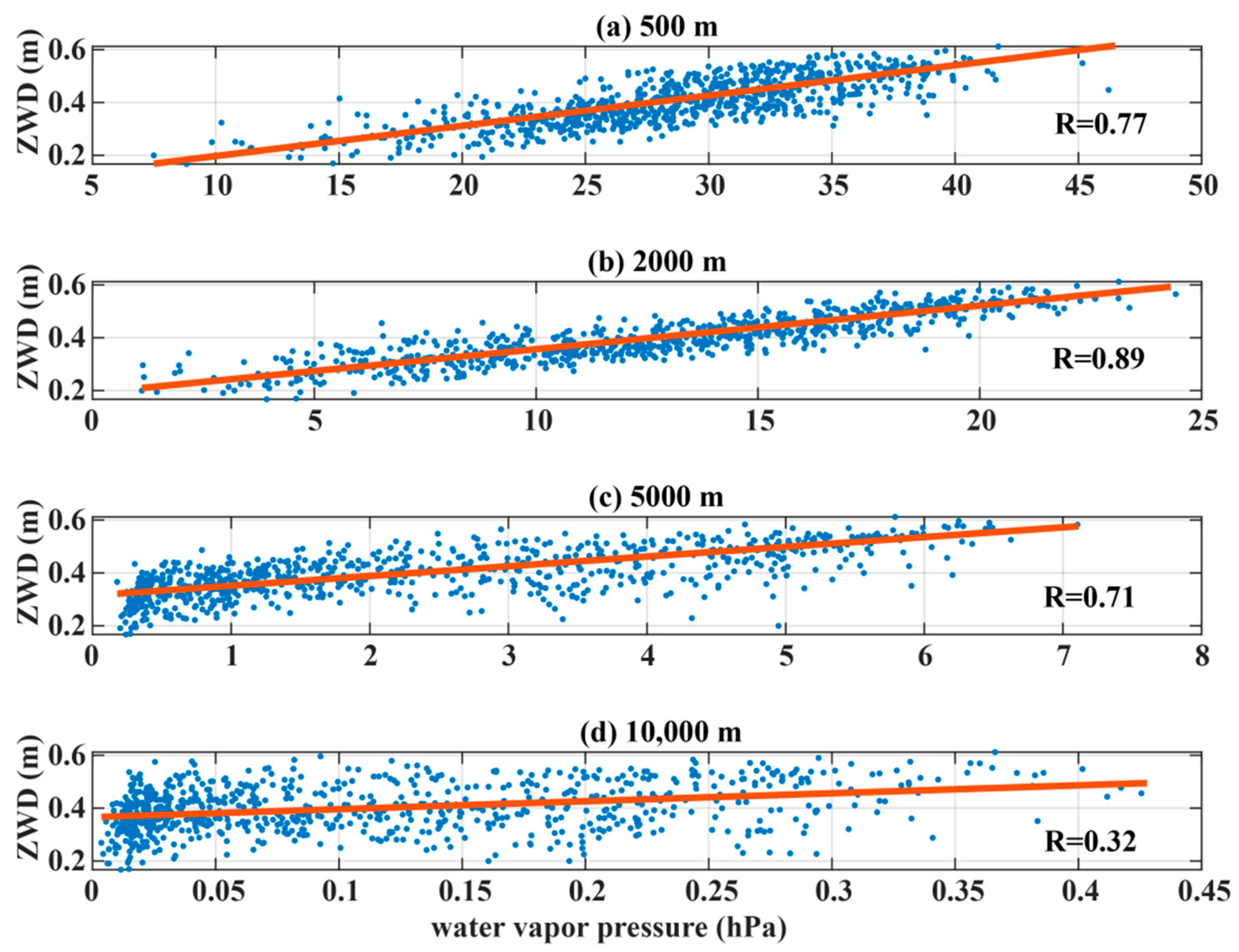
Figure 2 indicates the statistical relationships between ZWD and water vapor pressure of Qingdao station at the height of 500, 2000, 5000, and 10,000 m, respectively. A well linear correlation was found between ZWD and water vapor pressure according to the figure, a stronger correlation was found at the lower height, and the correlation decreases with increase of height, this is due to the fact that most water vapor exists in the lower atmosphere and the water vapor density as well as water vapor pressure decrease with height.

To investigate the variation characteristic of the correlation between zenith wet delay and water vapor pressure further, over 10 years’ (through 2008 to 2017) radiosonde meteorological data of China Big-Triangle Points, Qingdao, Sanya, Kashi, and Jiamusi stations with the different months were processed and analyzed, respectively.

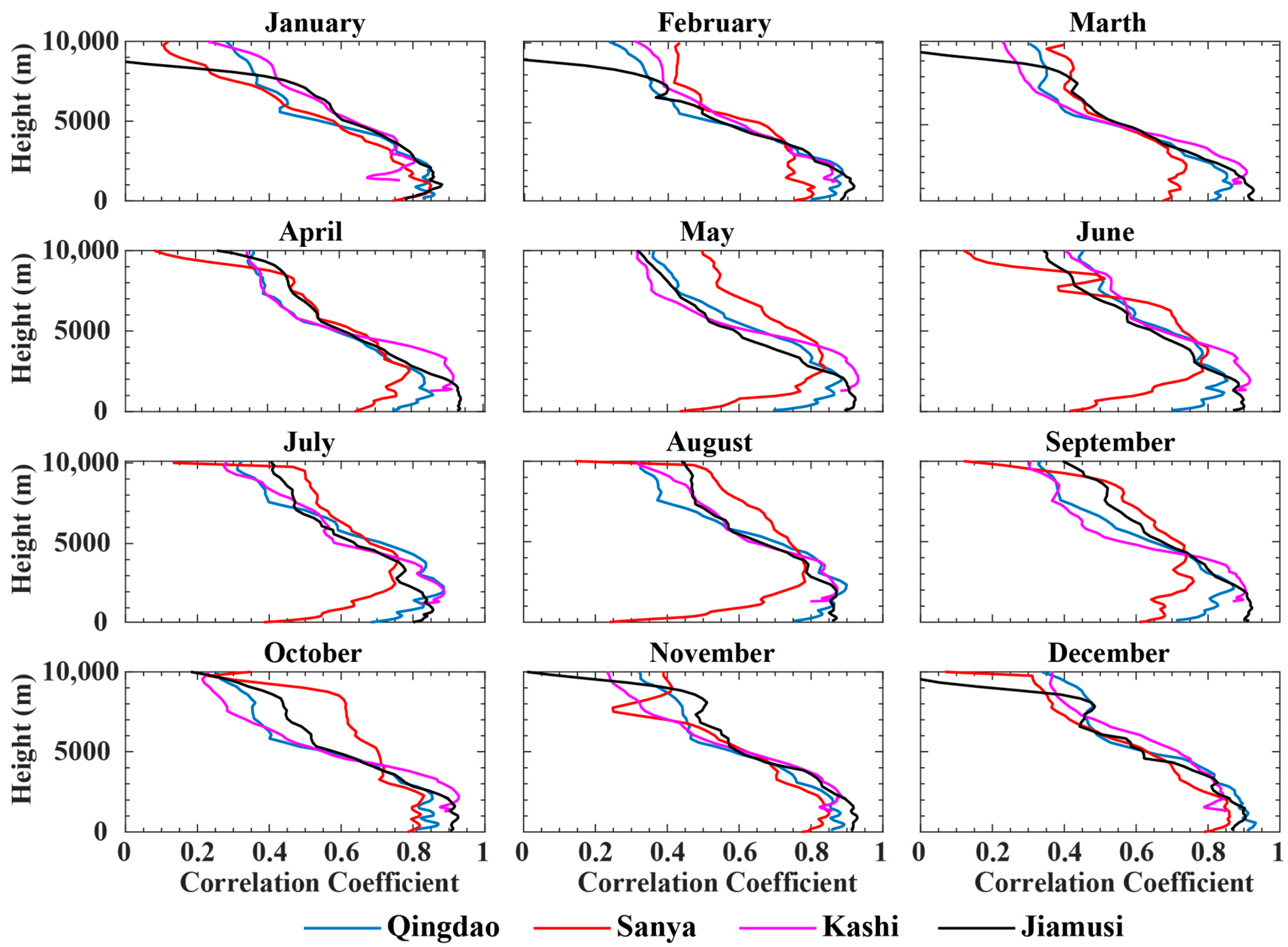
Figure 3 depicts the variations of the correlation coefficients with height between zenith wet delay and water vapor pressure at different months of Qingdao, Sanya, Kashi, and Jiamusi stations, respectively.

Table A1. Correlation coefficients between zenith wet delay and water vapor pressure of Qingdao station at different heights and months.

Month	Height (m)
	526	1026	2076	3076	4076	5076	7076	10,076
January	0.85	0.83	0.85	0.75	0.71	0.53	0.39	0.28
February	0.87	0.87	0.88	0.76	0.69	0.52	0.36	0.24
Marth	0.84	0.86	0.84	0.74	0.65	0.52	0.34	0.30
April	0.81	0.86	0.84	0.75	0.68	0.58	0.42	0.36
May	0.82	0.86	0.88	0.80	0.77	0.65	0.47	0.36
June	0.79	0.84	0.85	0.76	0.77	0.68	0.53	0.46
July	0.77	0.83	0.89	0.82	0.82	0.71	0.50	0.32
August	0.83	0.86	0.90	0.82	0.81	0.69	0.45	0.34
September	0.79	0.83	0.87	0.80	0.75	0.63	0.44	0.34
October	0.87	0.86	0.85	0.77	0.70	0.55	0.36	0.25
November	0.89	0.88	0.86	0.76	0.71	0.57	0.45	0.32
December	0.93	0.91	0.89	0.89	0.82	0.78	0.62	0.46

,

Table A2. Correlation coefficients between zenith wet delay and water vapor pressure of Sanya station at different heights and months.

Month	Height (m)
	507	1107	2007	3007	4007	5007	7007	10,007
January	0.84	0.84	0.78	0.74	0.66	0.58	0.38	0.12
February	0.80	0.79	0.75	0.75	0.72	0.65	0.47	0.43
Marth	0.70	0.72	0.73	0.70	0.65	0.54	0.41	0.40
April	0.70	0.76	0.77	0.75	0.71	0.64	0.51	0.08
May	0.57	0.75	0.79	0.82	0.82	0.76	0.61	0.50
June	0.49	0.62	0.74	0.78	0.80	0.73	0.57	0.12
July	0.54	0.64	0.72	0.74	0.76	0.68	0.56	0.13
August	0.51	0.66	0.73	0.78	0.78	0.74	0.66	0.14
September	0.68	0.68	0.74	0.72	0.74	0.72	0.61	0.12
October	0.82	0.82	0.82	0.73	0.72	0.70	0.62	0.35
November	0.83	0.85	0.83	0.73	0.69	0.62	0.40	0.39
December	0.86	0.86	0.85	0.74	0.70	0.63	0.42	0.06

,

Table A3. Correlation coefficients between zenith wet delay and water vapor pressure of Kashi station at different heights and months.

Month	Height (m)
	1290	1540	2090	2990	4040	5040	7040	10,040
January	0.76	0.68	0.77	0.74	0.74	0.63	0.46	0.22
February	0.85	0.83	0.85	0.75	0.69	0.59	0.41	0.31
Marth	0.87	0.87	0.91	0.83	0.71	0.53	0.32	0.23
April	0.85	0.89	0.92	0.89	0.80	0.59	0.41	0.34
May	0.88	0.91	0.93	0.90	0.82	0.62	0.39	0.31
June	0.87	0.89	0.91	0.88	0.81	0.67	0.56	0.40
July	0.82	0.86	0.89	0.82	0.76	0.58	0.52	0.28
August	0.80	0.84	0.87	0.84	0.78	0.62	0.52	0.32
September	0.87	0.88	0.90	0.88	0.78	0.55	0.41	0.31
October	0.89	0.88	0.93	0.88	0.74	0.55	0.33	0.23
November	0.85	0.82	0.87	0.85	0.76	0.61	0.40	0.23
December	0.84	0.79	0.84	0.82	0.77	0.71	0.48	0.37

and

Table A4. Correlation coefficients between zenith wet delay and water vapor pressure of Jiamusi station at different heights and months.

Month	Height (m)
	482	1032	1932	3082	4082	5082	7082	10,082
January	0.83	0.88	0.85	0.79	0.72	0.60	0.50	−0.19
February	0.89	0.92	0.88	0.79	0.67	0.54	0.40	−0.25
Marth	0.91	0.92	0.88	0.77	0.66	0.55	0.42	−0.12
April	0.93	0.93	0.90	0.78	0.70	0.60	0.49	0.24
May	0.92	0.91	0.89	0.78	0.68	0.58	0.44	0.31
June	0.90	0.89	0.88	0.76	0.73	0.64	0.48	0.34
July	0.84	0.85	0.83	0.77	0.74	0.63	0.47	0.40
August	0.86	0.86	0.87	0.79	0.75	0.64	0.50	0.44
September	0.91	0.92	0.90	0.81	0.76	0.66	0.54	0.39
October	0.91	0.92	0.90	0.78	0.69	0.57	0.45	0.16
November	0.92	0.93	0.90	0.83	0.72	0.59	0.49	−0.02
December	0.88	0.90	0.86	0.83	0.73	0.62	0.46	−0.10

in the Appendix A present the correlation coefficients at typical heights from January to December of those stations. We can find that the similar variation trend was shown in Figure 3, and there is strong correlation for heights less than 5000 km and almost all the correlation coefficients are greater than 0.6.

3.1.2. Estimation of Zenith Wet Delay (ZWD) by GNSS Precise Point Positioning

Due to the atmospheric refraction, GNSS signals propagating through the Earth’s atmosphere are slightly lengthened with retarded speeds, and the delays of GNSS signals are called the neural atmospheric delay and ionospheric delay in the ionosphere, which were considered as a nuisance and error source for a long time, while nowadays these delays could be extracted and transformed into the useful atmospheric parameters. After being passed through the atmosphere into the ground, GNSS signals carry a large amount of atmospheric information. Therefore, GNSS precise point positioning (PPP) [26] can be used to detect tropospheric information as well as positioning. Here, a ground-based GNSS method is used to calculate the ZWD as follows:

Firstly, ZTD is computed by GPS zero-differenced observation combinations, given by Equation (9):

$$\{\begin{array}{l}P=\rho +c(d_t-d_T)+T_{trop}+T_{iono}+{\epsilon }_P\\ \phi =\rho +c(d_t-d_T)+T_{trop}-T_{iono}+N\times \lambda +{\epsilon }_{\phi }\end{array}$$

(9)

where:

$P$: code pseudorange measurements of two frequencies (m);

$\phi$: phase pseudorange measurements of two frequencies (L1, L2), respectively (m);

$\rho$: the distance between satellite and antenna of GPS receiver (m);

$c$: the speed of light (m/s);

$dt$: the receiver clock error (s);

$dT$: the satellite clock error (s);

$T_{trop}$: the signal delay caused by atmosphere (m);

$T_{iono}$: the signal delay caused by ionosphere (m);

N: the integer ambiguity (cycle);

$\lambda$: the wavelength of carrier phase (m);

${\epsilon }_P$: is the code error containing remaining errors, such as multipath and noise (m);

${\epsilon }_{\phi }$: is the phase error containing remaining errors, such as multipath and noise (m).

As $T_{trop}$ is the slant tropospheric delay along the signal path from the satellite to the receiver, each satellite with a different elevation angle corresponds to a different slant tropospheric delay (STD), a mapping relationship given by Equation (10):

$$T_{trop}=\mathrm{ZTD}\cdot M$$

(10)

where M is the mapping function of tropospheric delays, the common mapping functions include Herring Mapping Function [27], Niell Mapping Function [28], Global Mapping Function [29], Vienna Mapping Function [30], etc. Herein, Global Mapping Function is recommended for use as it provides better precision than the Niell Mapping Function and smaller height biases with respect to Vienna Mapping Function, and it can be easy to implement because it only needs input parameters of station coordinates and day of year [29].

Secondly, ZHD is calculated by an empirical model based on ground surface pressure given by Equation (7).

Lastly, the ZWD can be obtained by subtracting ZHD from ZTD.

3.1.3. Building Inversion Model by Intelligent Optimization Algorithm

For the inversion process of the profile of water vapor pressure, first of all, forward calculation of input and output parameters should be carried out, that is, the tropospheric path delay ZWD should be calculated by ray-tracing algorithm [31,32] based on the known atmospheric parameter profile:

$$\begin{array}{l}\mathrm{ZWD}={\displaystyle {\int }_{r0}^{r_T}(n_w-1)}csc\theta dr={10}^{-6}{\displaystyle {\int }_{r0}^{r_T}{N}_{w}csc\theta dr}\\ ={10}^{-6}{\displaystyle {\int }_{r0}^{r_T}(3.73\times {10}^5\frac{e_w}{T^2})}csc\theta dr\end{array}$$

(11)

where $\theta$ is elevation of the signal path, it denotes zenith wet delay when its value equals to 90 degree. $n_w$ and $N_w$ are the wet term of atmospheric refractive index and refractivity respectively, $e_w$ and T are water vapor pressure and temperature, respectively.

Then the inversion network can be built based on a large number of historical meteorological data. As there is a well linear correlation between water vapor pressure and zenith wet delay, one can build the relationship between the profile of water vapor pressure and ZWD. The inversion network should be trained by using a large number of historical meteorological data based on an intelligent optimization algorithm such as Neural Network [33], Support Vector Machine [34], Relevance Vector Machine (RVM) [21], etc. Here, we chose RVM to train the inversion network, because it has a number of advantages, which include the benefits of probabilistic predictions, automatic estimation of parameters, and the facility to utilize arbitrary basis functions, which are not necessary to be ‘Mercer’ kernels. The key feature of RVM is that as well as offering good generalization performance, the inferred predictors are exceedingly sparse in that they contain relatively few non-zero $w_i$ parameters. The majority of parameters are automatically set to zero during the learning process, giving a procedure that is extremely effective at discerning those basis functions that are ‘relevant’ for making good predictions.

The training of RVM is conducted under the Bayesian framework, which can be used for regression estimation and prediction to obtain the distribution of predicted values, given by:

$$y(x,w)={\displaystyle \sum _{i=1}^N{w}_{i}K(x,x_i)+w_0}$$

(12)

where $K(x,x_i)$ is the function of kernels, $w_i$ is the weight coefficients of the model, the output is a linearly-weighted sum of N, generally nonlinear and fixed, basis functions $K(x,x_i)$. With a wide domain of convergence and its applications to a variety of situations, Gaussian kernel function is usually used in RVM algorithm, which can be expressed by the following equation:

$$K(x_1,x_2)=\exp (-\Vert x_1-x_2\Vert /{\sigma }^2)$$

(13)

where $\sigma$ is width parameter, $\Vert ·\Vert$ denotes the norm of vector. Here, $\sigma$ is taken as the standard deviation of the input training data vector, the input vector X is given by:

$$X=[T,P,E_w,\mathrm{ZWD}]$$

(14)

where T, P, E_w are the ground surface atmospheric temperature, pressure and water vapor pressure of historical meteorological data, respectively, ZWD is calculated by Equation (11).

Normalize all data according to size range, and take standard deviation of normalized vector inner product:

$$\sigma =std\langle X,X\rangle$$

(15)

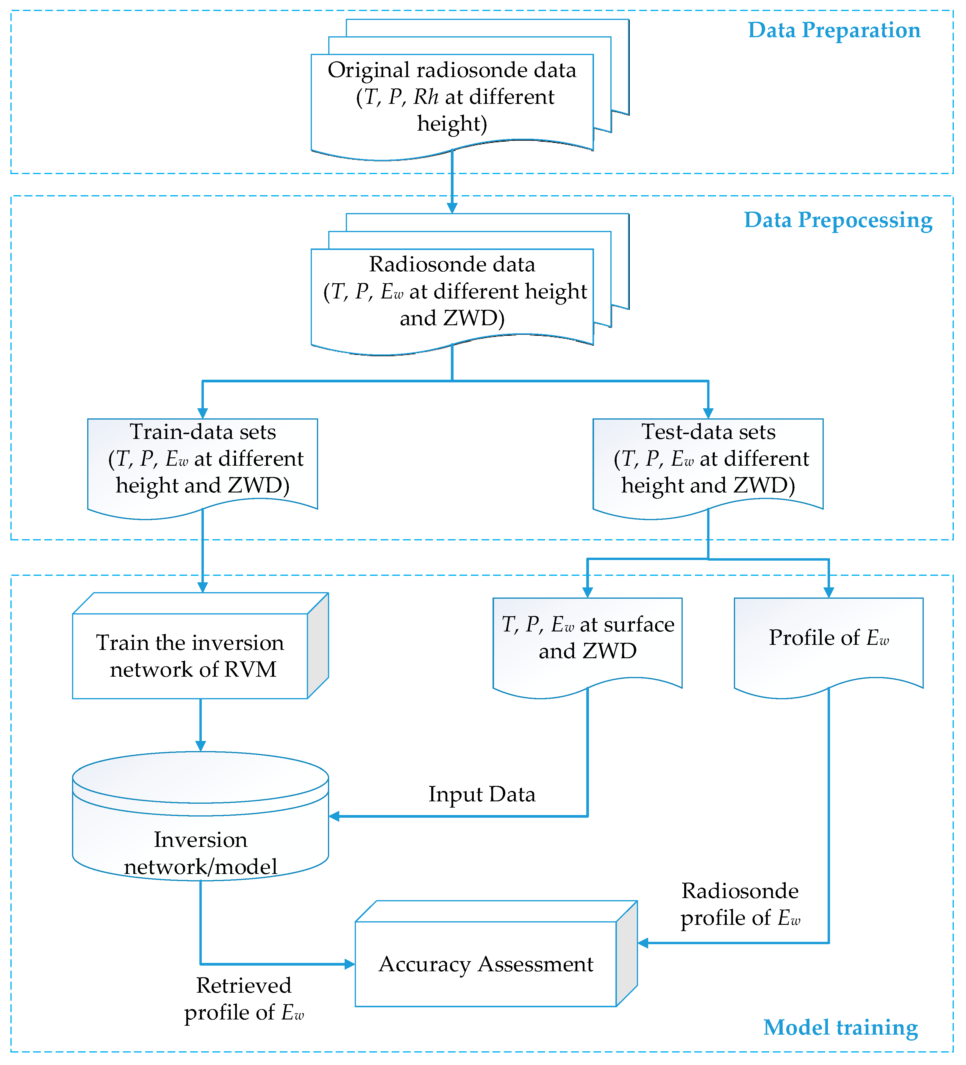
The inversion network training procedure is shown in Figure 4 and can be built by these steps as follows:

• The radiosonde data including atmospheric temperature, relative humidity, pressure, and height should be extracted from years of original radiosonde data. Then, we can obtain the water vapor pressure $E_w$ by Equation (8) and calculate ZWD by Equation (11).
• Divide all the data mentioned in step 1 into two parts: the train-data sets and the test-data sets, of which the proportion is 90 and 10 percent, respectively.
• Train the inversion network of RVM based on the train-data sets by adjusting the key parameters such as function of kernels, weight coefficients, and normalization variables.
• By putting surface temperature, water vapor pressure, pressure, and ZWD of test-data sets into inversion network built in step 3, we can get the retrieved profile of water vapor pressure. The accuracy of the model can be evaluated by comparing the retrieved profile of water vapor pressure with radiosonde profile of water vapor pressure. An accuracy threshold is set as 7 N-unit here, if the accuracy is enough, the modeling procedure is over, otherwise step 3 will be repeated until the error expectation is reached.

Figure 4. Flow diagram of training procedure for retrieving profile of water vapor pressure.

Figure 4. Flow diagram of training procedure for retrieving profile of water vapor pressure.

3.1.4. Retrieving the Profile of Water Vapor Pressure Based on GNSS Measurement

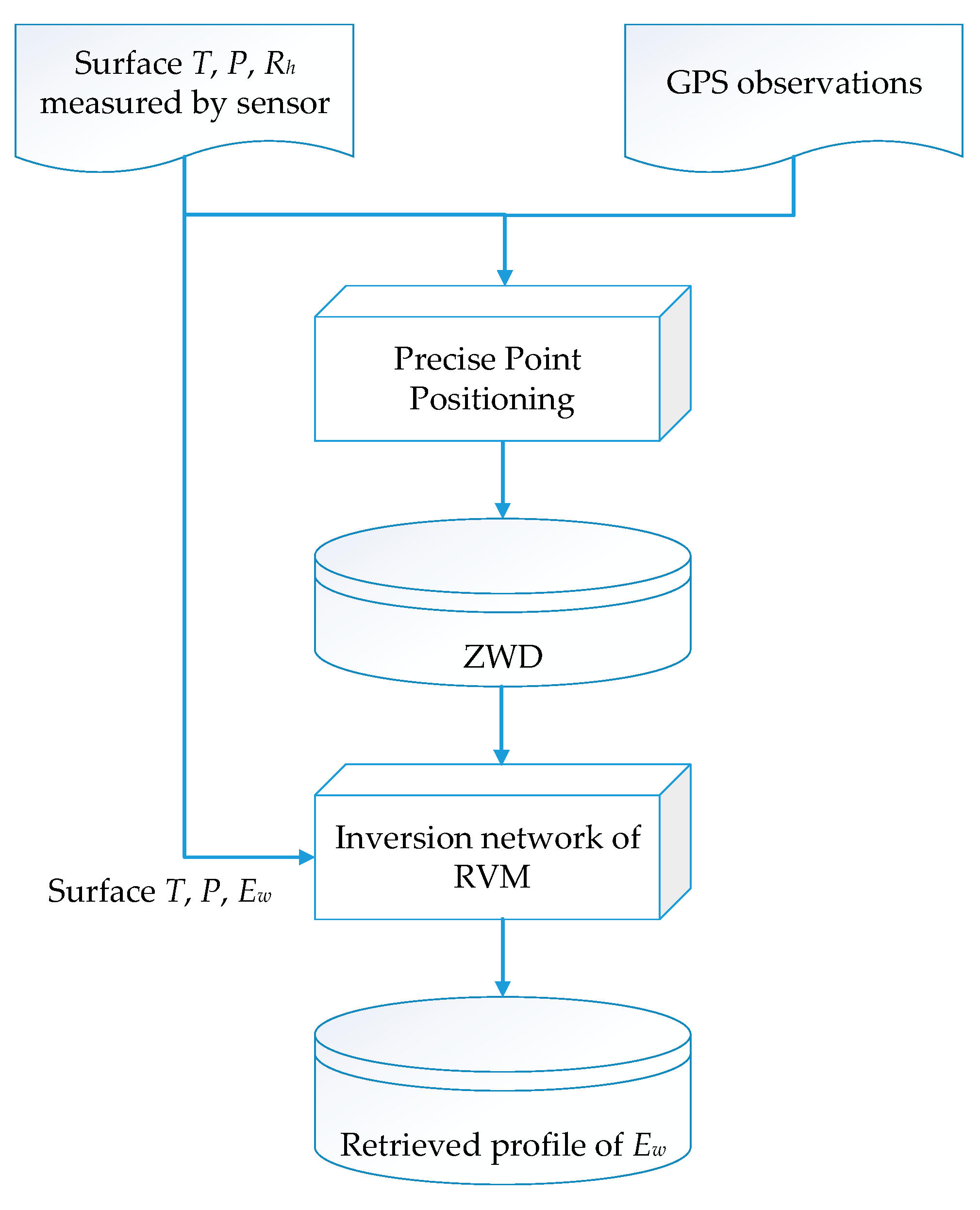
Once the inversion model has been built, water vapor pressure can be retrieved in real time based on original measurement of single ground-based GNSS and meteorological sensor. The flow diagram for retrieving tropospheric refractivity is shown in Figure 5. Firstly, the original GNSS observed data and broadcast ephemeris are collected by GNSS receiver, and the surface meteorological data is collected by meteorological sensor. Secondly, measurement data based on precise point positioning algorithm introduced in Section 3.1.2. are processed. As a result, the ZWD will be obtained. Thirdly, by inputting the ZWD, T, E_w, and P at the surface to the inversion model, we can get the profile of water vapor pressure.

3.1.5. Inversion Examples and Analysis

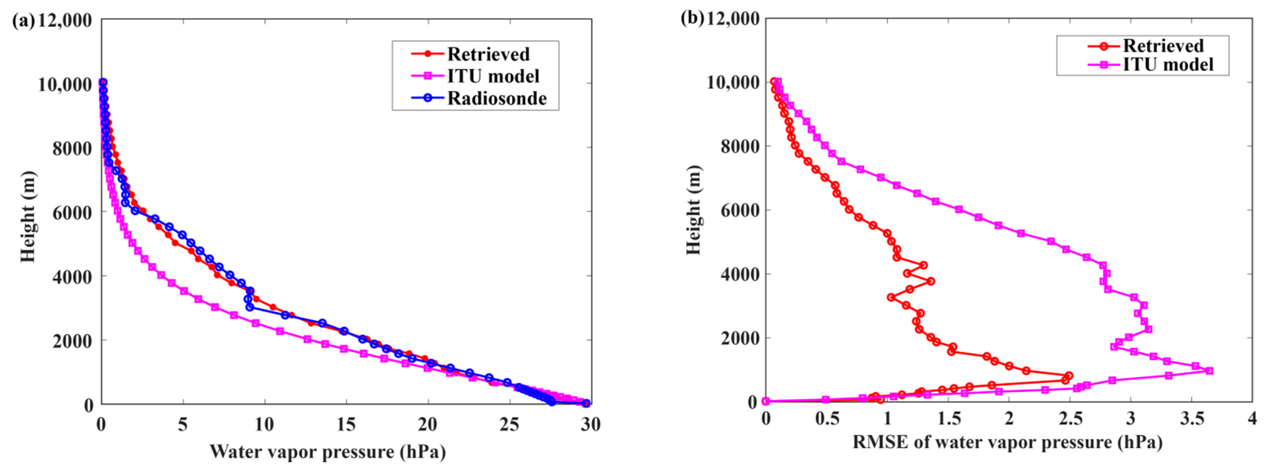
The inversion network of Sanya was built based on the method introduced in Section 3.1.3 and 10 years’ historical meteorological data from 2008 to 2017 of Sanya radiosonde station was conducted as modeling data. The GPS observation data of 2017 at Sanya station was used to retrieve the pressure of water vapor and compare to radiosonde results as well as ITU model. A typical comparison result of the profile of water vapor pressure between retrieved, ITU model, and radiosonde is shown in Figure 6a.

It can be seen that the radiosonde water vapor pressure varies irregularly along the height. Although the retrieved results have a significant error at some heights, the variation trend in the whole height layer is in good agreement with the radiosonde data. Statistics showed that the average water vapor content of Sanya station in the layers up to 3 and 5 km were 91.61 and 97.58%, respectively. Figure 6b shows the root mean square error between the radiosonde and the retrieved profile of water vapor pressure of those input data and the maximum error of water vapor pressure of retrieved and ITU model can reach about 2.5 and 3.7 hPa respectively, and the mean of RMSE of water vapor pressure of retrieved and ITU model over the whole height are about 1.1 and 1.9 hPa, respectively.

3.2. Fitted Temperature and Pressure Profile of Reference Model

The distribution of atmospheric temperature with altitude is more regular and stable than that of water vapor pressure. Different models of atmospheric temperature distribution are selected according to different geographical locations and seasons, the least square method is used to fit the coefficients of the polynomial model based on a large numbers of historical meteorological radiosonde data of local stations. The temperature does not change obviously with the season in low-latitude area, the distribution model of temperature is given by [35]:

$$\{\begin{array}{ll}T(h)=T_0+a\cdot h^2+b\cdot h+c& 0\le h\le h_1\\ T(h)=T_1+d\cdot (h-h_1)& h_1\le h\le h_2\\ T(h)=T_2& h_2\le h\le h_3\end{array}$$

(16)

In summer of mid-latitude and high-latitude area, the atmospheric temperature profile model of different heights is expressed by:

$$\{\begin{array}{ll}T(h)=T_0+a\cdot h^2+b\cdot h+c& 0\le h\le h_1\\ T(h)=T_1& h_1\le h\le h_2\\ T(h)=T_2\exp [d\cdot (h-h_2)]& h_2\le h\le h_3\\ T(h)=T_3& h_3\le h\le h_4\end{array}$$

(17)

In winter of mid-latitude area, the atmospheric temperature profile model of different heights is expressed by:

$$\{\begin{array}{ll}T(h)=T_0+a\cdot h^2+b\cdot h+c& 0\le h\le h_1\\ T(h)=T_1& h_1\le h\le h_2\\ T(h)=T_2+d\cdot (h-h_2)& h_2\le h\le h_3\\ T(h)=T_3& h_3\le h\le h_4\end{array}$$

(18)

In winter of high-latitude area, the atmospheric temperature profile model of different heights is expressed by:

$$\{\begin{array}{ll}T(h)=T_0+a\cdot h^3+b\cdot h^2+c\cdot h+d& 0\le h\le h_1\\ T(h)=T_1& h_1\le h\le h_2\\ T(h)=T_2+e\cdot (h-h_2)& h_2\le h\le h_3\\ T(h)=T_3& h_3\le h\le h_4\end{array}$$

(19)

where $T_0$ is the temperature of ground surface (K); $T_1$, $T_2$, $T_3$ are temperature of height $h_1$, $h_2$, $h_3$, respectively; $h_1$, $h_2$, $h_3$, $h_4$ are top height of troposphere, isothermal layer, thermal inversion layer, and second isothermal layer, respectively; $h$ is height (km); $a$, $b$, $c$, $d$, $e$ are fitting coefficients of historical radiosonde data of different areas and months.

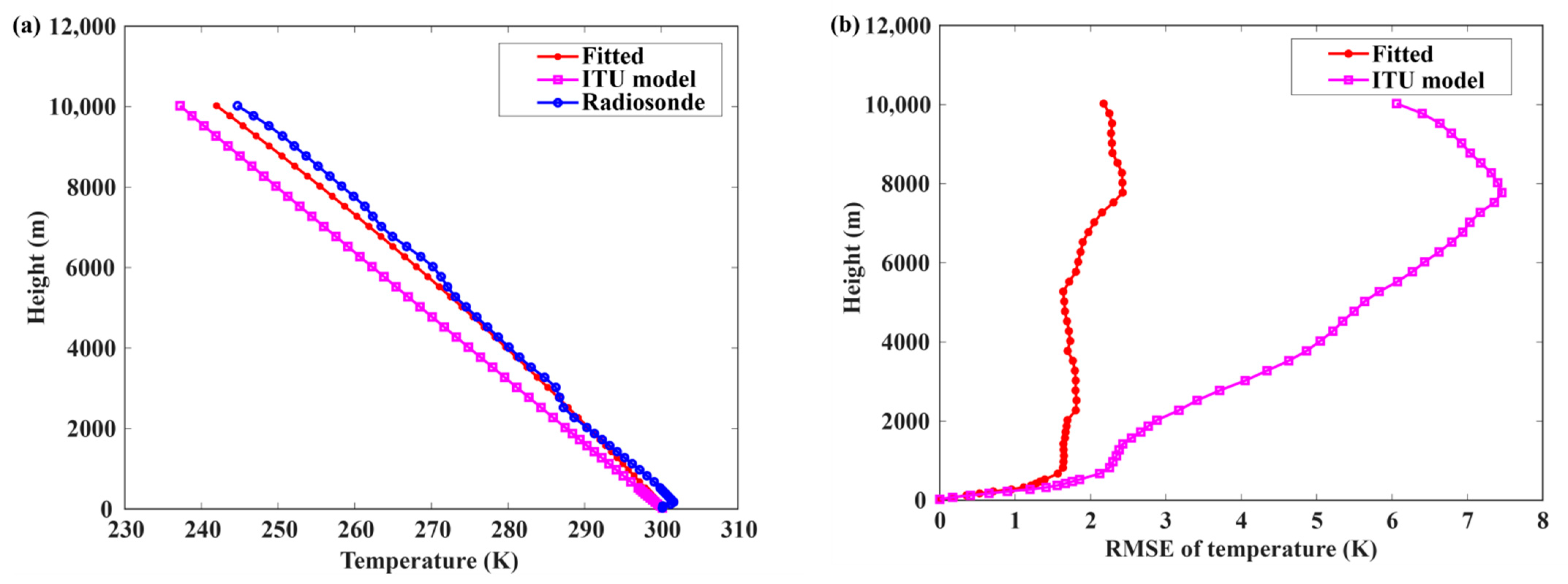
According to the definition of the least square method, the polynomial coefficient was calculated by historical temperature radiosonde data of years so that the sum of the squares of deviations at each point was minimized, then the temperature model was built. A typical comparison result of temperature profile between fitted and radiosonde is shown in Figure 7.

It can be seen that the variation of temperature profile is more regular and stable than that of water vapor pressure, the variation trend of the fitted temperature profile shows a good agreement with the radiosonde data. In order to validate the accuracy of the fitted method, 50 test-data sets were input to the network, Figure 7b shows the root mean square error of fitted and ITU model temperature compared to radiosonde temperature, the biggest temperature error of fitted and ITU model can reach over 2.4 and 7.4 K respectively, the mean RMSE of temperature of fitted and ITU model over the whole height are about 1.7 and 4.3 K, respectively.

The variation of pressure $P(h)$ with height is calculated by the following formula based on the temperature profile:

$$\{\begin{array}{l}P(h)=P_i{[\frac{T_i}{T_i+L_i(h-H_i)}]}^{34.163/L_i}{L}_i\ne 0\\ P(h)=P_i\exp (\frac{-34.163(h-H_i)}{T_i})L_i=0\end{array}$$

(20)

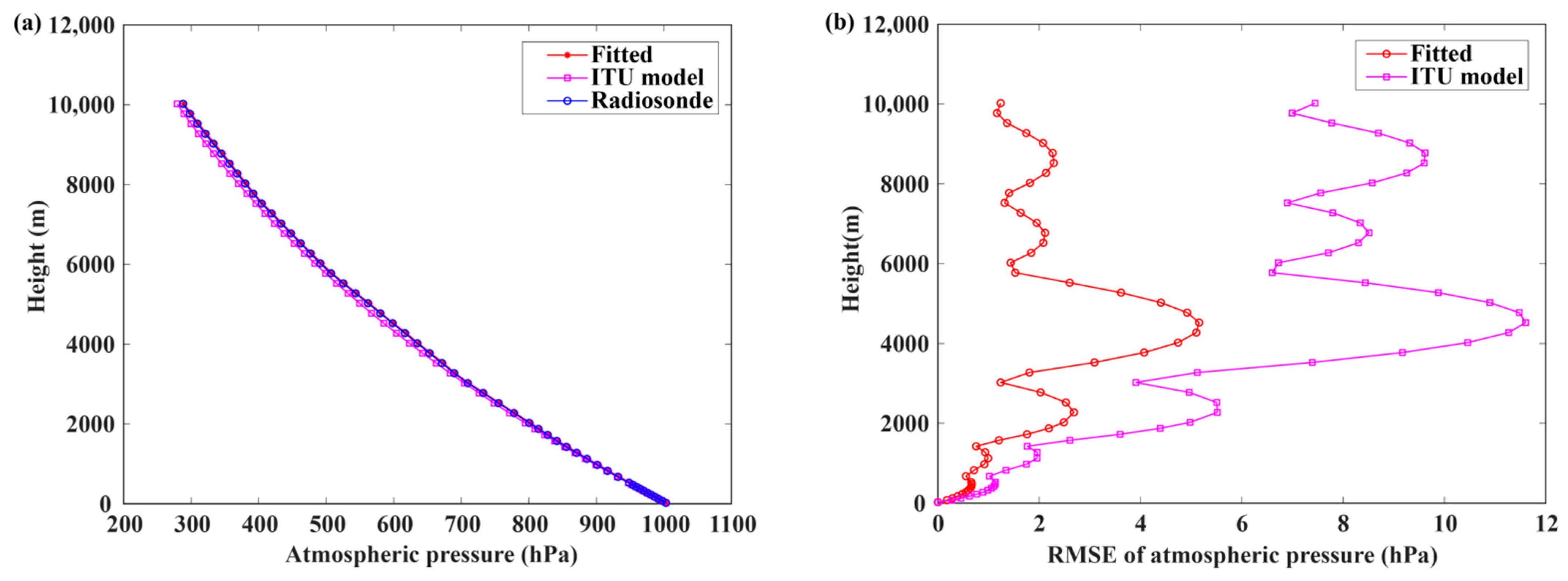
where $P_i$, $T_i$, $L_i$ are the pressure (hPa), temperature (K), and gradient of temperature (K/km) of the ith height layer, respectively. Figure 8 shows the comparison between fitted, ITU model, and radiosonde atmospheric pressure profile and the root mean square error of fitted pressure profile and ITU model pressure profile. The distribution of pressure with height is most stable compared to water vapor pressure and temperature profile, the mean RMSE of pressure calculated by fitted and ITU model over the whole height are about 2.2 and 5.6 hPa, respectively.

4. Results and Discussion

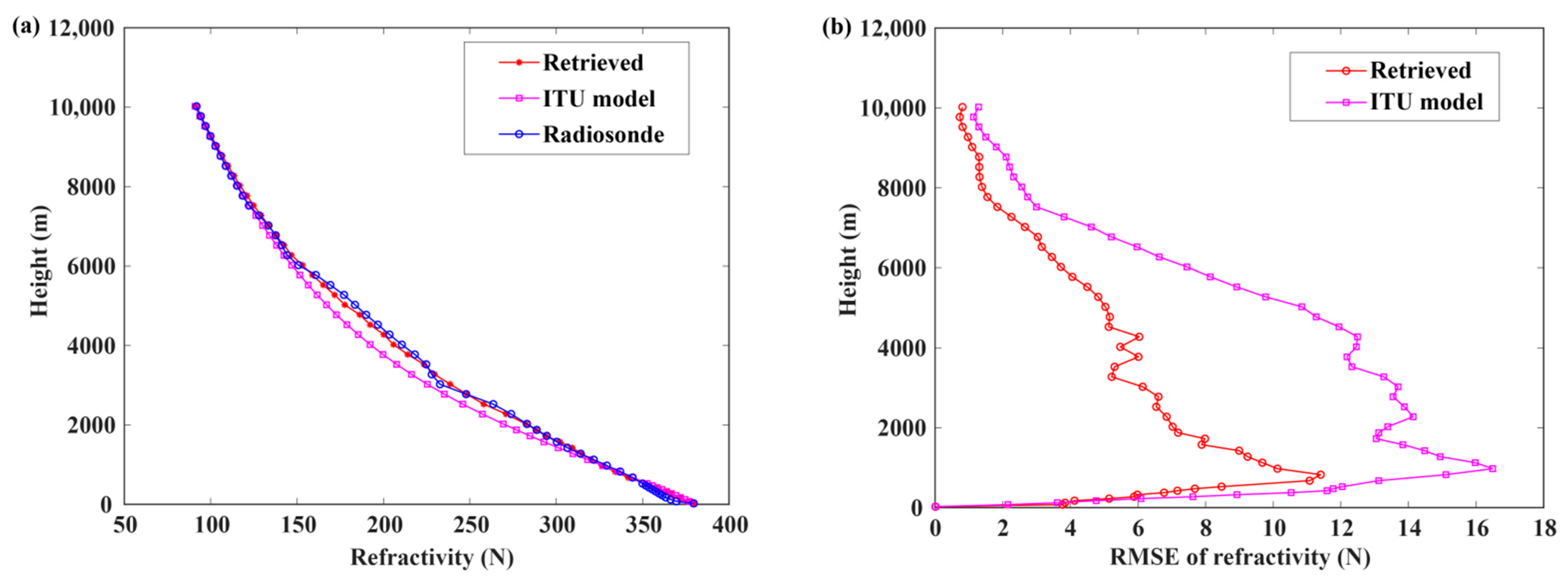
The retrieval refractivity profile can be obtained by Equation (3) after the profile of water vapor pressure, temperature profile, and pressure profile is calculated. Figure 9 shows the comparison between fitted, ITU model, and radiosonde refractivity profile and the RMSE of retrieved refractivity profile and ITU model refractivity profile. The mean RMSE of refractivity calculated by retrieved and ITU model over the whole height are about 5.3 and 8.5 N-unit, respectively.

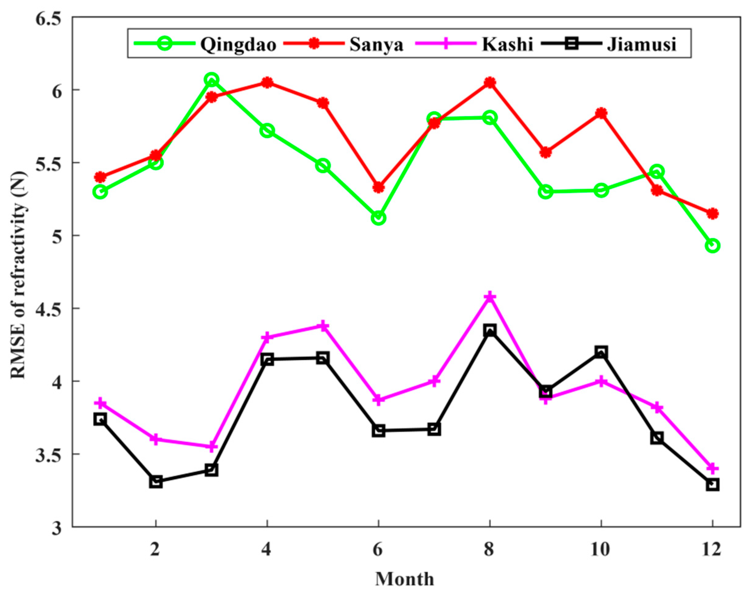
To verify the effectiveness of the proposed method further, ten years’ historical meteorological data from 2008 to 2017 of Qingdao, Sanya, Kashi, and Jiamusi radiosonde stations for different months were used to build the inversion model. GPS observations of 2017 at these four stations were conducted to retrieve the refractivity and validate the accuracy, as shown in Figure 10, the annual average error of the proposed method at Qingdao, Sanya, Kashi, and Jiamusi are about 5.48, 5.63, 3.58, and 3.78 N-unit, respectively.

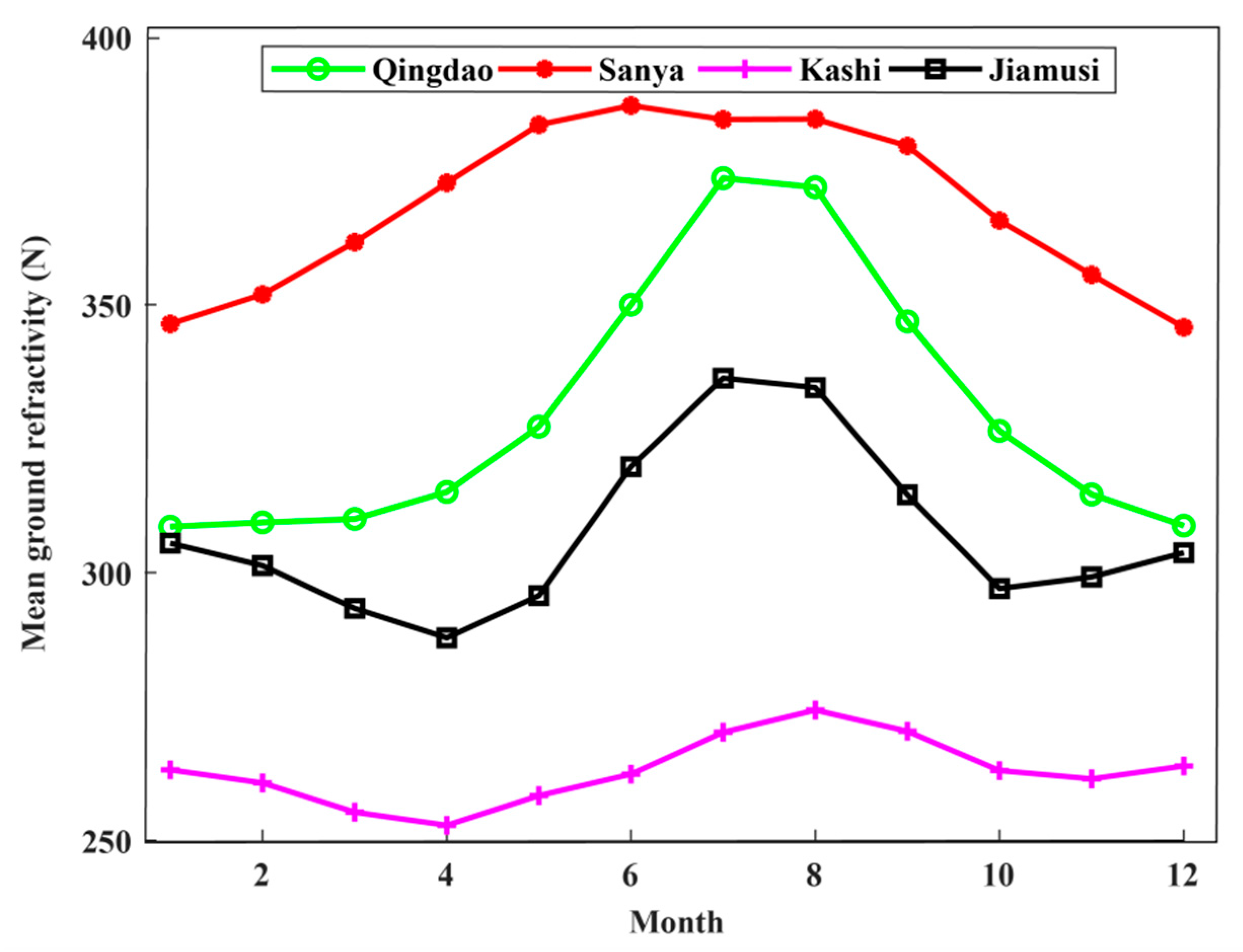
The RMSE of Qingdao and Sanya station are relatively larger than that of Kashi and Jiamusi stations, this is because they have different climatic peculiarities. Qingdao and Sanya stations are located in the north temperate monsoon coastal region and the low latitude coastal region with a tropical ocean monsoon climate, respectively, while Kashi and Jiamusi stations are located in a warm temperate continental arid climate zone and the middle temperate humid climate zone with a continental monsoon climate, respectively. As is shown by Figure 11 and Figure 12, the ground surface refractivity is generally higher in the summertime than in the wintertime, the ground surface refractivity of Qingdao and Sanya station are relatively larger than that of Kashi and Jiamusi station.

Figure 13 shows the relative RMSE of refractivity profile of these four stations mentioned above in different months, which ranges from 1.1 to 2%, and the annual average relative RMSE of refractivity of the proposed method at Qingdao, Sanya, Kashi, and Jiamusi are about 1.66, 1.53, 1.49, and 1.23%, respectively.

5. Conclusions

In this study, we proposed a method for retrieving low tropospheric refractivity profile from GPS measurement. While the hydrostatic part is larger than the wet part, the wet refractivity is much more variable and difficult to estimate, the variability of atmospheric refractivity is mainly attributed to the wet part, which accounts for about 10–30% of the entire refractive index. In previous studies and recommendations, this term is estimated from an empirical formula, which induced large errors. By analyzing the variations of the correlation between zenith wet delay and water vapor pressure based on over ten years’ radiosonde meteorological data at Qingdao, Sanya, Kashi, and Jiamusi stations with different months, we found that there is a good linear correlation between zenith wet delay and water vapor pressure at different heights. The correlation decreases with increase of height due to the fact that water vapor mainly exists in the lower troposphere and the water vapor density as well as water vapor pressure rapidly decreasing with height. So we can build the relationship between the profile of water vapor pressure and ZWD, estimation of zenith tropospheric delay from GPS measurement is capable of providing accurate ZWD. We can retrieve water vapor pressure profile based on ZWD and the inversion model. By integrating the temperature and pressure profile adopted by reference atmosphere, we compared our results of atmospheric refractivity with the radiosonde measurement at China Big-Triangle Points, Qingdao, Sanya, Kashi, and Jiamusi station with a ten-year dataset. The RMSE of refractivity of the proposed method at Qingdao, Sanya, Kashi, and Jiamusi are about 5.48, 5.63, 3.58, and 3.78 N-Unit, respectively, and the annual average relative RMSE of refractivity of the proposed method at these stations are about 1.66, 1.53, 1.49, and 1.23%, respectively. This proposed method is very promising for radio meteorology research and atmospheric radio wave propagation correction for aerospace measurement and control.

References

1. Shikhovtsev, A.Y.; Kovadlo, P.G.; Bol’Basova, L.A.; Lukin, V.P. Features of the Formation of Wavefront Slopes on the Telescope Aperture at Different Vertical Profiles of Optical Atmospheric Turbulence. Atmos. Ocean. Opt. 2020, 33, 141–145. [Google Scholar] [CrossRef]
2. Bettouche, Y.; Obeidat, H.; Agba, B.; Kouki, A.; Alhassan, H.; Rodriguez, J.; Abd-Alhameed, R.; Jones, S. Long-Term Evolution of The Surface Refractivity for Arctic Regions. Radio Sci. 2019, 54, 602–611. [Google Scholar] [CrossRef] [Green Version]
3. Kovadlo, P.G.; Lukin, V.P.; Shikhovtsev, A.Y. Development of the Model of Turbulent Atmosphere at the Large Solar Vacuum Telescope Site as Applied to Image Adaptation. Atmos. Ocean. Opt. 2019, 32, 202–206. [Google Scholar] [CrossRef]
4. Matsumoto, H. The Refractive Index of Moist Air in the 3-μm Region. Metrologia 1982, 18, 49–52. [Google Scholar] [CrossRef]
5. Lowry, A.R.; Rocken, C.; Sokolovskiy, S.V.; Anderson, K.D. Vertical profiling of atmospheric refractivity from ground-based GPS. Radio Sci. 2002, 37, 1–21. [Google Scholar] [CrossRef]
6. Doerry, A.W. Earth Curvature and Atmospheric Refraction Effects on Radar Signal Propagation; Sandia National Laboratories: Albuquerque, NM, USA, 2013; pp. 15–20.
7. Ovodenko, V.; Trekin, V.; Korenkova, N.; Klimenko, M. Investigating range error compensation in UHF radar through IRI-2007 real-time updating: Preliminary results. Adv. Space Res. 2015, 56, 900–906. [Google Scholar] [CrossRef]
8. Tang, T.; Liu, G.; Liu, L. Numerical modeling the propagation path of radio waves with atmospheric refractivity. Microw. Opt. Technol. Lett. 2020, 62, 1651–1655. [Google Scholar] [CrossRef]
9. Hopfield, H.S. Two-quartic tropospheric refractivity profile for correcting satellite data. J. Geophys. Res. 1969, 74, 4487–4499. [Google Scholar] [CrossRef]
10. Bean, B.R.; Thayer, G.D. Models of the Atmospheric Radio Refractive Index. Proc. IRE 1959, 47, 740–755. [Google Scholar] [CrossRef]
11. Kämpfer, N.; Nedoluha, G.; Haefele, A.; Dewachter, E. Monitoring Atmospheric Water Vapour; Springer: New York, NY, USA, 2013; pp. 3–5. [Google Scholar]
12. Torres, B.; Cachorro, V.E.; Toledano, C.; Ortiz-De-Galisteo, J.P.; Berjón, A.J.; De Frutos, A.M.; Bennouna, Y.; Laulainen, N. Precipitable water vapor characterization in the Gulf of Cadiz region (southwestern Spain) based on Sun photometer, GPS, and radiosonde data. J. Geophys. Res. 2010, 115, 1–11. [Google Scholar] [CrossRef] [Green Version]
13. Kuznetsov, A.; Seroukhova, O.; Simakina, T.; Kryukova, S. The vertical profile of the refraction coefficient for microwave radiation in the troposphere and its variability. J. Phys. Conf. Ser. 2021, 1991, 012008. [Google Scholar] [CrossRef]
14. Dong, X.; Yang, L.; Zhu, Q.; Guo, C.; Zhao, Z.; Lin, L. A Method of Retrieving Tropospheric Refractivity Above Ocean Surface using GNSS. In Proceedings of the 2018 12th International Symposium on Antennas, Propagation and EM Theory (ISAPE), Hangzhou, China, 3–6 December 2018; pp. 1–4. [Google Scholar]
15. Liao, Q.; Sheng, Z.; Shi, H. Joint Inversion of Atmospheric Refractivity Profile Based on Ground-Based GPS Phase Delay and Propagation Loss. Atmosphere 2016, 7, 12. [Google Scholar] [CrossRef] [Green Version]
16. Trzcina, E.; Rohm, W. Estimation of 3D wet refractivity by tomography, combining GNSS and NWP data: First results from assimilation of wet refractivity into NWP. Q. J. R. Meteorol. Soc. 2019, 145, 1034–1051. [Google Scholar] [CrossRef]
17. Lin, L.; Zhao, Z.; Zhang, Y.; Zhu, Q. Tropospheric refractivity profiling based on refractivity profile model using single ground-based global positioning system. IET Radar Sonar Navig. 2011, 5, 7–11. [Google Scholar] [CrossRef]
18. Perler, D.; Geiger, A.; Hurter, F. 4D GPS water vapor tomography: New parameterized approaches. J. Geod. 2011, 85, 539–550. [Google Scholar] [CrossRef] [Green Version]
19. Niell, A.E.; Coster, A.J.; Solheim, F.S.; Mendes, V.B.; Toor, P.C.; Langley, R.B.; Upham, C.A. Comparison of Measurements of Atmospheric Wet Delay by Radiosonde, Water Vapor Radiometer, GPS, and VLBI. J. Atmos. Ocean. Tech. 2001, 18, 830–850. [Google Scholar] [CrossRef] [Green Version]
20. Tipping, M. Sparse Bayesian Learning and the Relevance Vector Machine. J. Mach. Learn. Res. 2001, 1, 211–244. [Google Scholar]
21. Chen, J.; Yang, S.; Tan, W.; Wang, J.; Chen, Q.; Zhang, Y. Recent Results of the Chinese CMONOC GNSS Network. In Proceedings of the ION 2017 Pacific PNT Meeting, Honolulu, HI, USA, 1–4 May 2017; pp. 539–546. [Google Scholar]
22. Nilsson, T.; Böhm, J.; Wijaya, D.D.; Tresch, A.; Nafisi, V.; Schuh, H. Path Delays in the Neutral Atmosphere; Springer: Berlin/Heidelberg, Germany, 2013; pp. 73–136. [Google Scholar]
23. Hill, R.J.; Lawrence, R.S.; Priestley, J.T. Theoretical and calculational aspects of the radio refractive index of water vapor. Radio Sci. 1982, 17, 1251–1257. [Google Scholar] [CrossRef]
24. Pikridas, C.; Katsougiannopoulos, S.; Zinas, N. A comparative study of zenith tropospheric delay and precipitable water vapor estimates using scientific GPS processing software and web based automated PPP service. Acta Geod. Geophys. 2014, 49, 177–188. [Google Scholar] [CrossRef]
25. Saastamoinen, J. Atmospheric Correction for the Troposphere and Stratosphere in Radio Ranging Satellites. In Use of Aritificial Satellites for Geodesy; Wiley: Hoboken, NJ, USA, 1972; Volume 15, pp. 247–251. [Google Scholar]
26. Zumberge, J.F.; Heflin, M.B.; Jefferson, D.C.; Watkins, M.M.; Webb, F.H. Precise point positioning for the efficient and robust analysis of GPS data from large networks. J. Geophys. Res. 1997, 102, 5005–5017. [Google Scholar] [CrossRef] [Green Version]
27. Herring, T. Modelling Atmospheric Delays in the Analysis of Space Geodetic Data. In Proceedings of the Symposium on Refraction of Transatmospheric Signals in Geodesy, The Hague, The Netherlands, 19–22 May 1992; pp. 157–164. [Google Scholar]
28. Neill, A.E. Global mapping for the atmospheric delay at radio wavelenghts. J. Geophys. Res. Atmos. 1996, 111, 3227–3246. [Google Scholar] [CrossRef]
29. Boehm, J.; Niell, A.; Tregoning, P.; Schuh, H. Global Mapping Function (GMF): A new empirical mapping function based on numerical weather model data. Geophys. Res. Lett. 2006, 33, 1–4. [Google Scholar] [CrossRef] [Green Version]
30. Kouba, J. Implementation and testing of the gridded Vienna Mapping Function 1 (VMF1). J. Geod. 2008, 82, 193–205. [Google Scholar] [CrossRef]
31. Mendes, V.B.; Langley, R.B. Tropospheric Zenith Delay Prediction Accuracy for High-Precision GPS Positioning and Navigation. Navigation 1999, 46, 25–34. [Google Scholar] [CrossRef]
32. Hobiger, T.; Ichikawa, R.; Koyama, Y.; Kondo, T. Fast and accurate ray-tracing algorithms for real-time space geodetic applications using numerical weather models. J. Geophys. Res. 2008, 113, 1–14. [Google Scholar] [CrossRef]
33. Narendra, K. Neural networks for control theory and practice. Proc. IEEE 1996, 84, 1385–1406. [Google Scholar] [CrossRef]
34. Vapnik, V.N. The Nature of Statistical Learning Theory; Springer: New York, NY, USA, 2000; pp. 138–146. [Google Scholar]
35. ITU-R. Recommendation ITU-R P.835-5: Reference Standard Atmospheres; ITU: Geneva, Switzerland, 2012. [Google Scholar]
Figure 1. The distribution of radiosonde meteorological stations.
Atmosphere 12 01468 g001
Figure 2. Statistical relationships between zenith wet delay and water vapor pressure at the height of (a) 500, (b) 2000, (c) 5000, and (d) 10,000 m, respectively.
Atmosphere 12 01468 g002
Figure 3. Variations of the correlation coefficients with height between zenith wet delay and water vapor pressure at different months of Qingdao, Sanya, Kashi, and Jiamusi station, respectively. The horizontal axis denote the correlation coefficients, the vertical axis denote heights in meters.
Atmosphere 12 01468 g003
Figure 5. Flow diagram for retrieving profile of water vapor pressure.
Atmosphere 12 01468 g005
Figure 6. (a) The comparison between the retrieved, ITU model and radiosonde profile of water vapor pressure; (b) The root mean square error of retrieved and ITU model profile of water vapor pressure.
Atmosphere 12 01468 g006
Figure 7. (a) The comparison between fitted, ITU model, and radiosonde temperature profile; (b) The root mean square error of fitted and ITU model temperature profile.
Atmosphere 12 01468 g007
Figure 8. (a) The comparison between fitted, ITU model, and radiosonde atmospheric pressure profile; (b) The RMSE of fitted and ITU model atmospheric pressure profile.
Atmosphere 12 01468 g008
Figure 9. (a) The comparison between fitted, ITU model, and radiosonde refractivity profile; (b) The root mean square error of fitted and ITU model refractivity profile.
Atmosphere 12 01468 g009
Figure 10. The RMSE of refractivity profile in different month.
Atmosphere 12 01468 g010
Figure 11. Boxplot of the ground refractivity in different months of 10 years’ radiosonde data, the red marks represent outlier data of refractivity.
Atmosphere 12 01468 g011
Figure 12. The mean ground refractivity in different months of 10 years’ radiosonde data.
Atmosphere 12 01468 g012
Figure 13. The relative RMSE of refractivity profile in different months.
Atmosphere 12 01468 g013