
Operational Analysis and Medium-Term Forecasting of the Greenhouse Gas Generation Intensity in the Cryolithozone

Abstract
:1. Introduction
- The data-driven predictive model is based on artificial intelligence methods and designed for operational estimation as well as for the formation of a forecast of the spatial concentration of greenhouse gases. This model allows for more accurate quantitative predictions of greenhouse gas generation because it relies on directly linking the measurements used to build the model to the measurement locations. This model is constantly being refined, literally at the rate of new data, and therefore takes into account the gradual depletion of hydrocarbon reserves in the soil, as well as this refinement gradually compensating for the a priori inaccuracy of hydrocarbon maps.
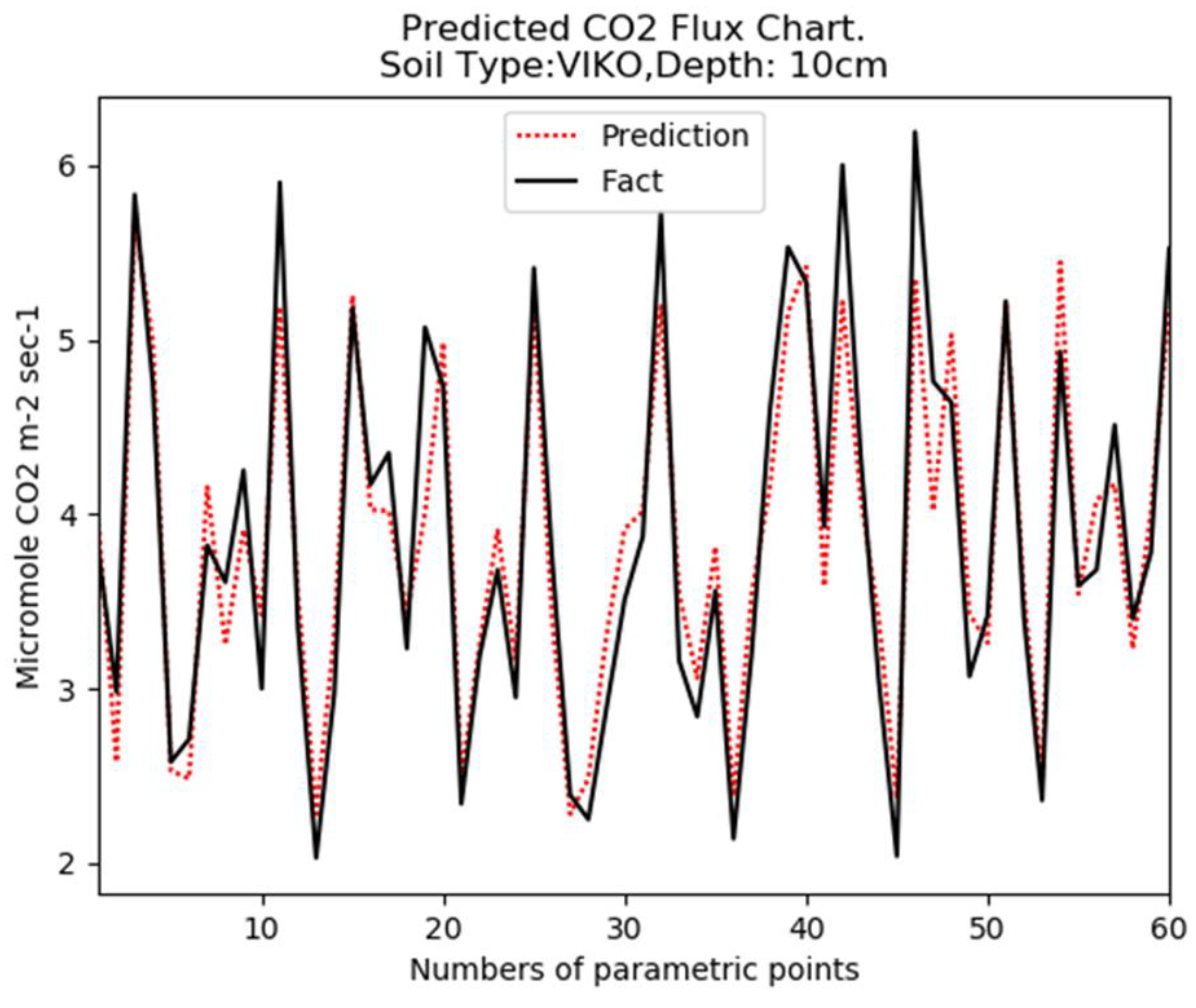
- The proof of the proposed predictive model adequacy was carried out in the form of numerical simulations with usage of a specialized data set.
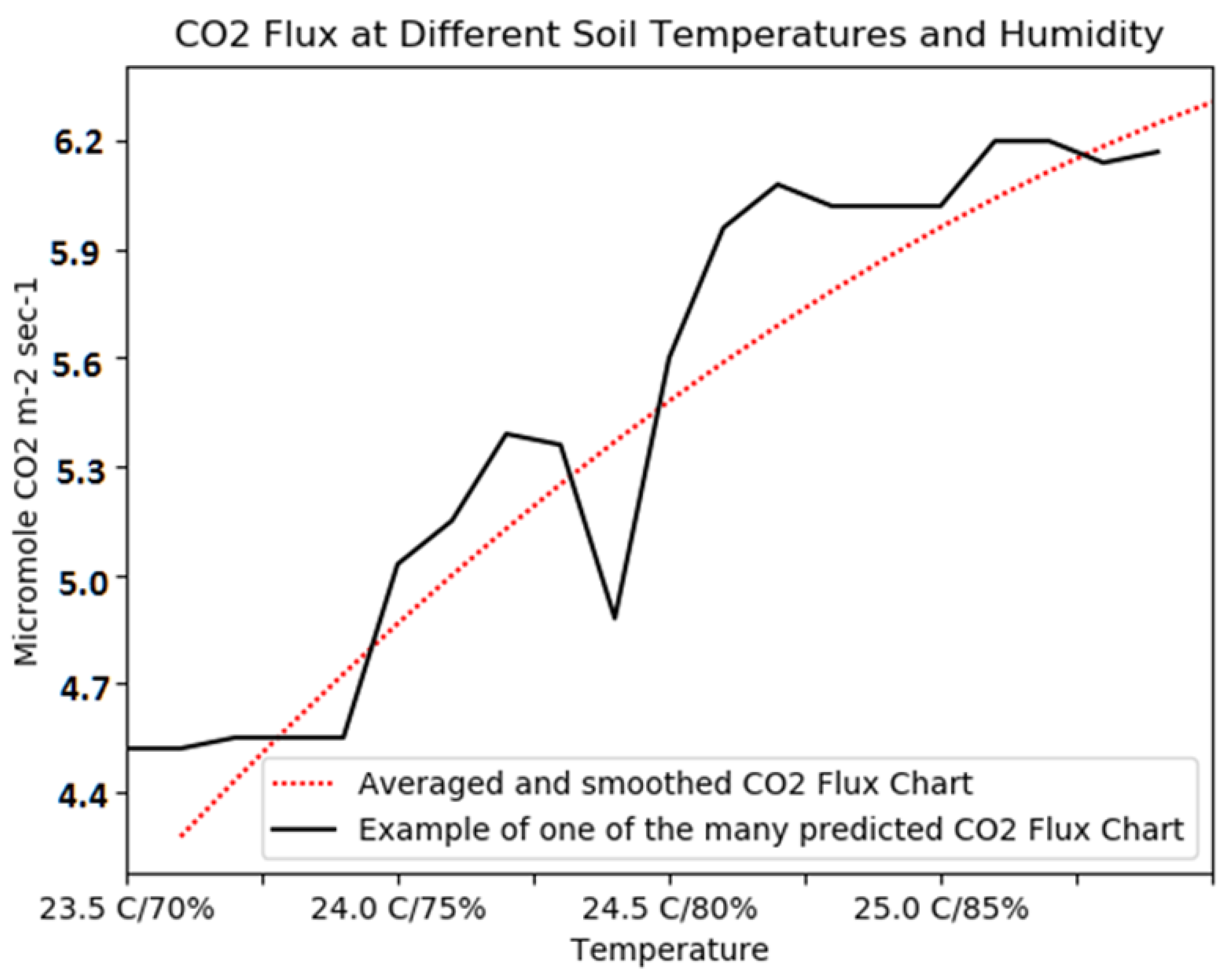
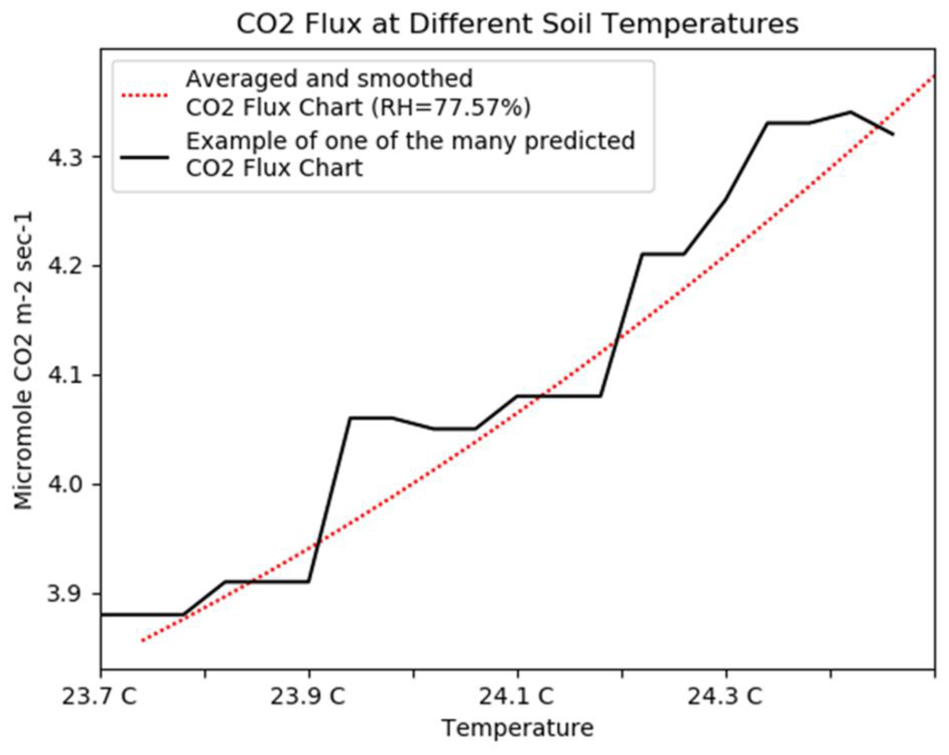
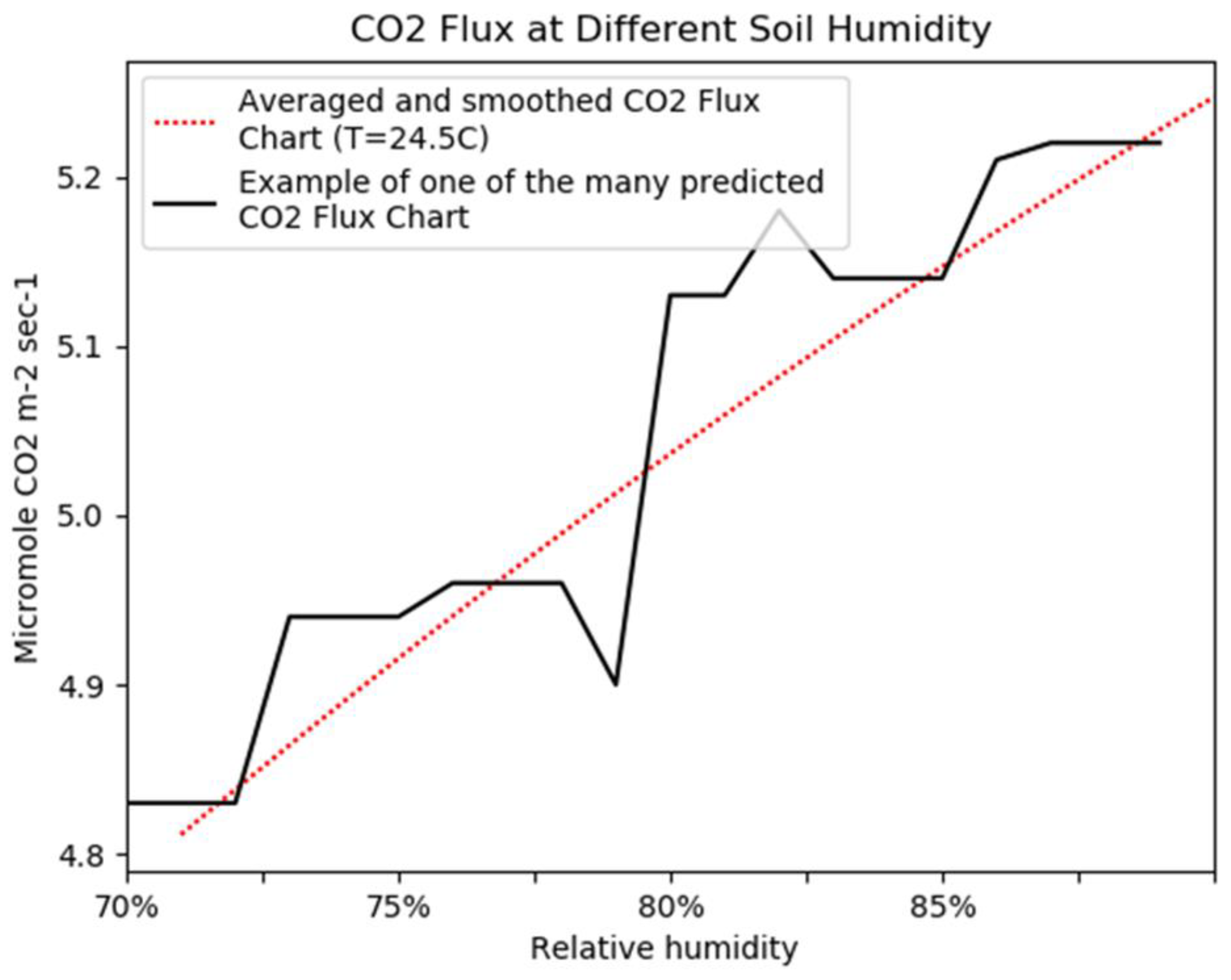
- The proof of existence of a sustainable regression model that binds the value of intensive CO2 production with the temperature and soil moisture was produced by numerical simulation.
2. Related Work
3. Method
4. Results
4.1. Description of the Data Set and Conditions for Numerical Studies
- Approximation method: GBR (Gradient Boosting Regression) [15].
- The available data set was always divided into two parts: the power of the first part 70%, and the power of the second part 30%. The first part was used for regression reconstruction, and the second part for testing. This was carried out in order to increase the generalizability of the approximation function. All results that summarize specific experiments always correspond to the test part of the sample only, according to the principle of cross validation.
- Several standard metrics were used to control the quality of approximation, including: MSE (mean squared error), explained_variance_score (explained variance regression score function, best possible score is 1.0, lower values are worse), max_error (maximum residual error), mean_absolute_error (mean absolute error regression loss), mean_squared_error (mean squared error regression loss), and r2_score (coefficient of determination regression, best possible score is 1.0). The metric r2_score was considered as dominant.
4.2. A Description of the Experimental Conditions and the Results Obtained in These Experiments
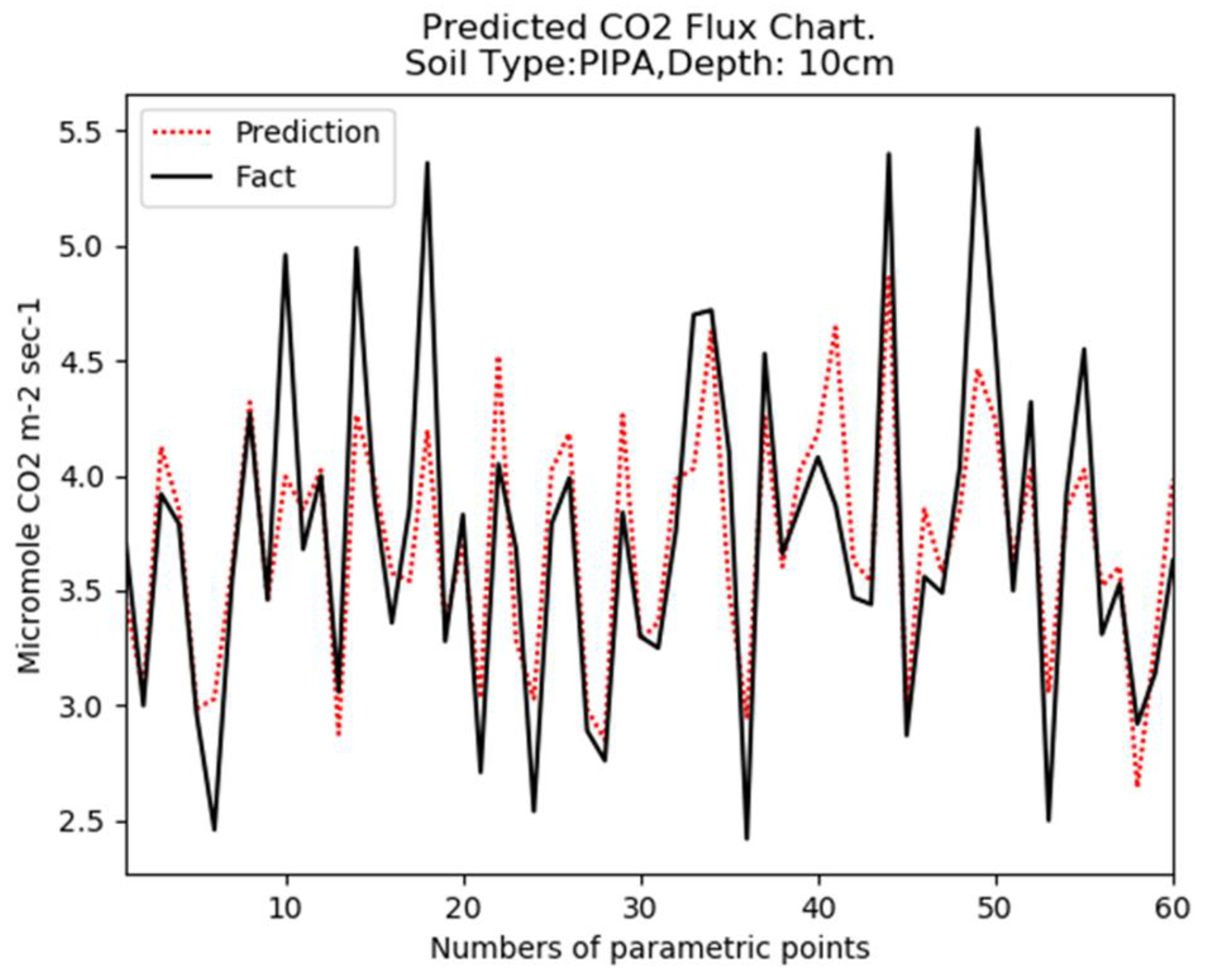
4.2.1. Experiment 1
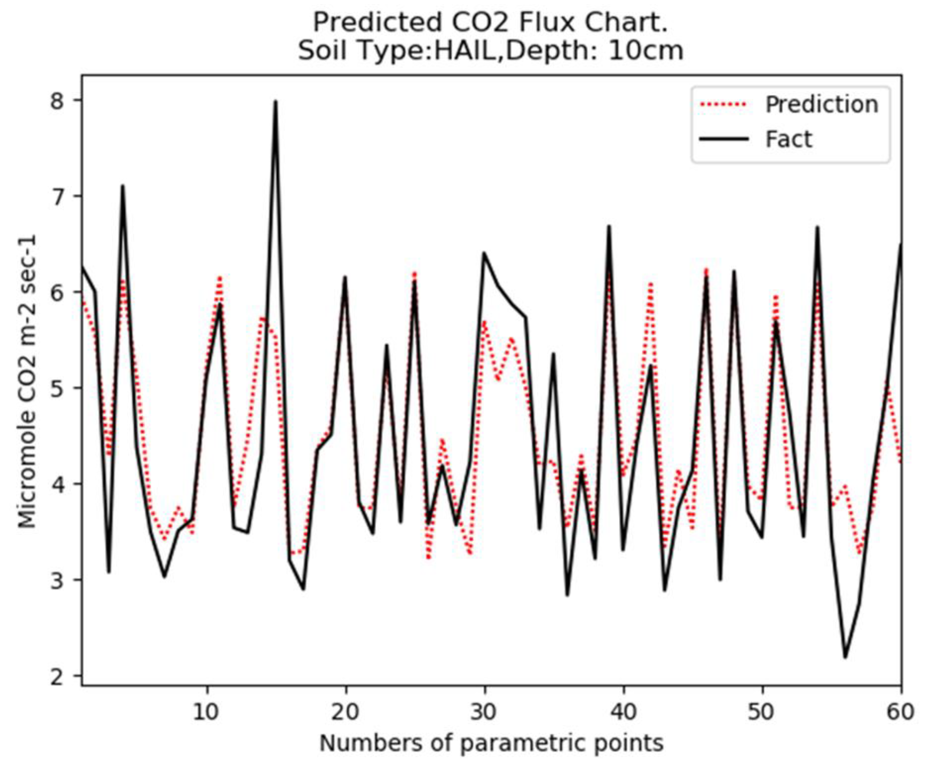
4.2.2. Experiment 2
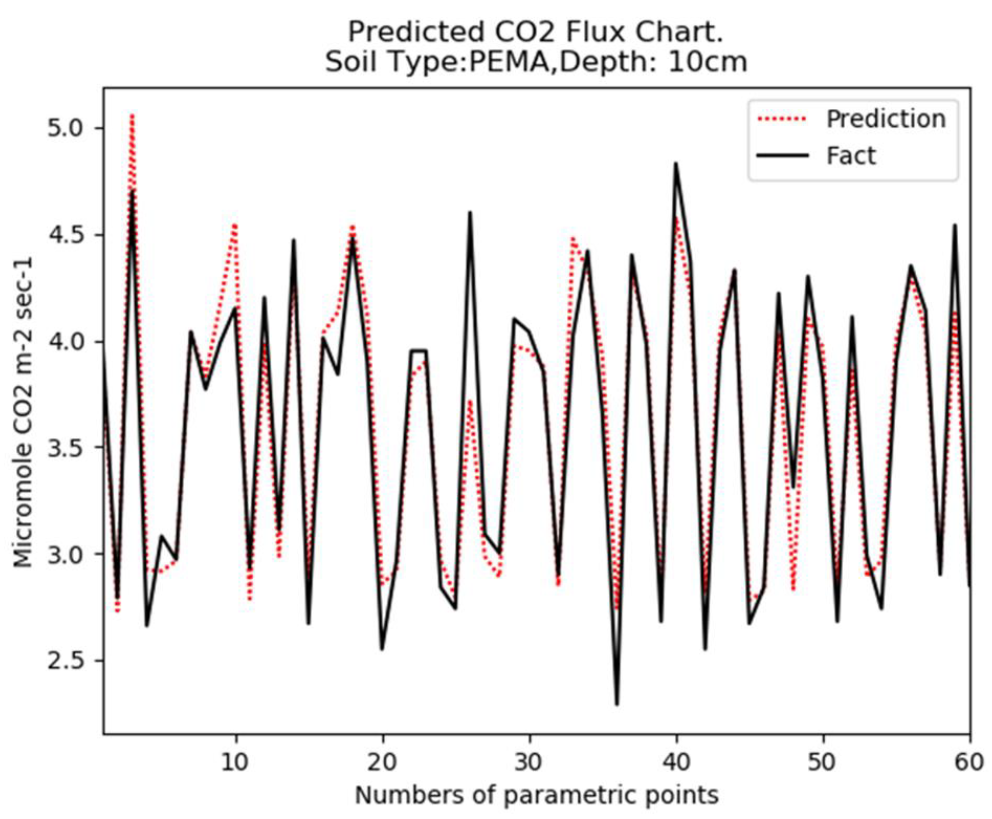
4.2.3. Experiment 3
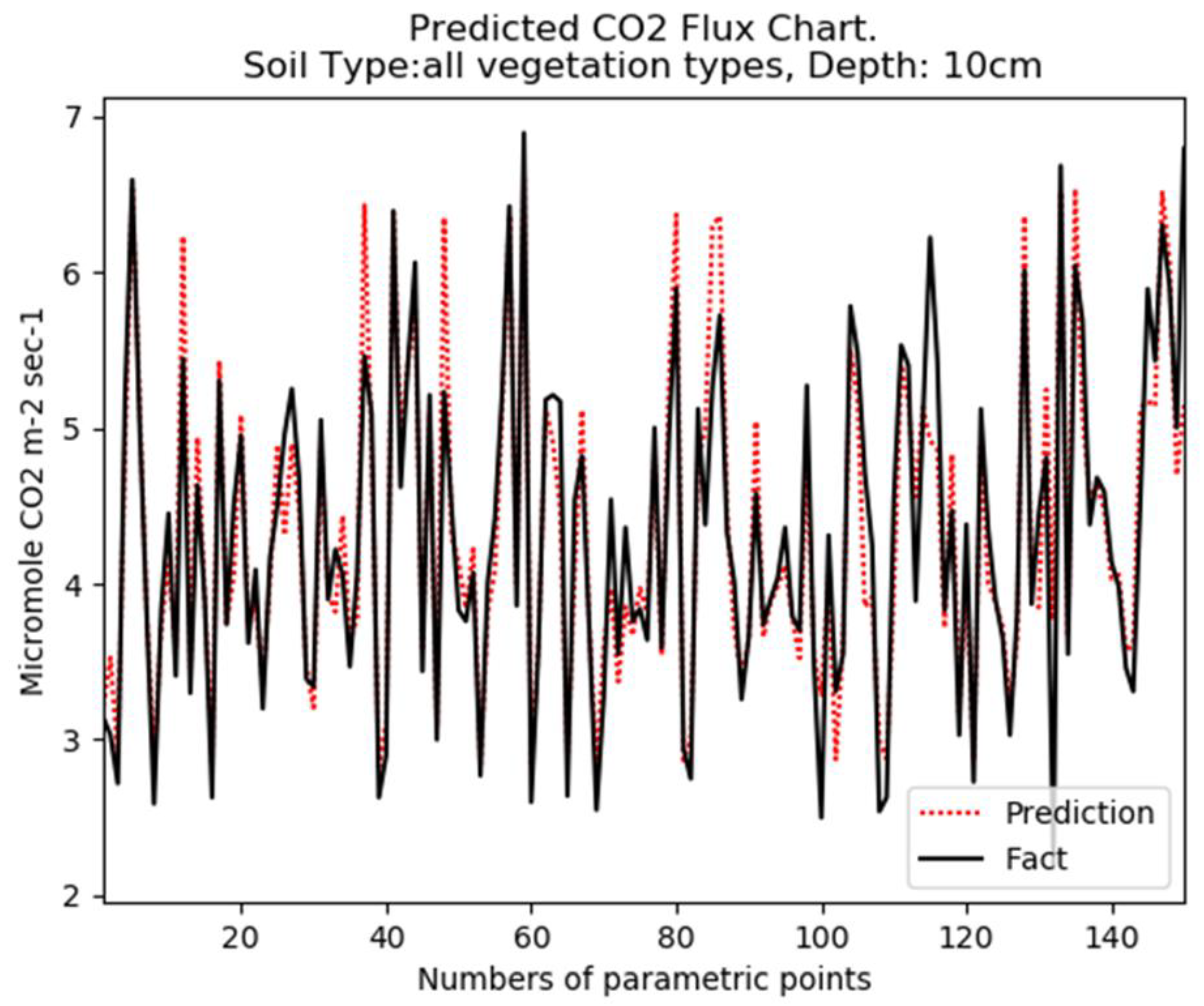
4.2.4. Experiment 4
4.2.5. Experiment 5
4.2.6. Experiment 6
4.2.7. Experiment 7
4.2.8. Experiment 8
5. Discussion on Numerical Simulations Results
6. Multimodal Measuring Stations (Multimodal Sensor Network) Requirements
- Each station must contain sensors for measuring CO2/CH4 flux, soil temperature, and soil moisture.
- The top-level data processing system, where information from the sensor network is collected, must contain information about the exact coordinate of the measurement points and about soil types at the measuring stations locations.
7. Conclusions
Author Contributions
Funding
Institutional Review Board Statement
Informed Consent Statement
Data Availability Statement
Conflicts of Interest
References
- Koven, C.D.; Ringeval, B.; Friedlingstein, P.; Ciais, P.; Cadule, P.; Khvorostyanov, D.; Krinner, G.; Tarnocai, C. Permafrost carbon-climate feedbacks accelerate global warming. Proc. Natl. Acad. Sci. USA 2011, 108, 14769–14774. [Google Scholar] [CrossRef] [PubMed] [Green Version]
- Vonk, J.; Sánchez, L.; García, B.; van Dongen, V.; Alling, V.; Kosm, A. Activation of old carbon by erosion of coas tal and subsea permafrost in Arctic Siberia. Nature 2018, 489, 137–140. [Google Scholar] [CrossRef] [PubMed]
- Turetsky, M.R.; Abbott, B.; Jones, M.C.; Anthony, K.W.; Olefeldt, D.; Schuur, E.A.G.; Koven, C.; McGuire, A.D.; Grosse, G.; Kuhry, P.; et al. Permafrost collapse is accelerating carbon release. Nature 2019, 569, 32–34. [Google Scholar] [CrossRef] [PubMed] [Green Version]
- Abbott, B.W.; Larouche, J.R.; Jones, J.B., Jr.; Bowden, W.B.; Balser, A.W. Elevated dissolved organic carbon biodegradability from thawing and collapsing permafrost. J. Geophys. Res. Biogeosci. 2014, 119, 2049–2063. [Google Scholar] [CrossRef]
- Schuur, E.A.G.; McGuire, A.D.; Schadel, C.; Grosse, G.; Harden, J.W.; Hayes, D.; Hugelius, G.; Koven, C.; Kuhry, P.; Lawrence, D.; et al. Climate change and the permafrost carbon feedback. Nature 2015, 520, 171–179. [Google Scholar] [CrossRef] [PubMed]
- Kraev, G.; Rivkina, E. Accumulation of Methane in Permafrost-Affected Soils of Cryolithozone. Arct. Environ. Res. 2017, 173–184. [Google Scholar] [CrossRef]
- Pries, C.E.H.; Logtestijn, R.S.P.; Schuur, E.A.G.; Natali, S.M.; Cornelissen, J.H.C.; Aerts, R.; Dorrepaal, E. Decadal warming causes a consistent and persistent shift from heterotrophic to autotrophic respiration in contrasting permafrost ecosystems. Glob. Chang. Biol. 2015, 21, 4508–4519. [Google Scholar] [CrossRef] [PubMed]
- Kwon, M.J.; Jung, J.Y.; Tripathi, B.M.; Göckede, M.; Lee, Y.K.; Kim, M. Dynamics of microbial communities and CO2 and CH4 fluxes in the tundra ecosystems of the changing Arctic. J. Microbiol. 2019, 57, 325–336. [Google Scholar] [CrossRef] [PubMed]
- Knoblauch, C.; Beer, C.; Liebner, S.; Grigoriev, M.N.; Pfeiffer, E.-M. Methane production as key to the greenhouse gas budget of thawing permafrost. Nat. Clim. Chang. 2018, 8, 309–312. [Google Scholar] [CrossRef] [Green Version]
- Kim, Y.; Ueyama, M.; Harazono, Y.; Tanaka, N.; Nakagawa, F.; Tsunogai, U. Assessment of Winter Fluxes of CO2 and CH4 in Boreal Forest Soils of Central Alaska Estimated by the Profile Method and the Chamber Method: A Diagnosis of Methane Emission and Implications for the Regional Carbon Budget. Tellus. Ser. B Chem. Phys. Meteorol. 2007, 59, 223–233. [Google Scholar] [CrossRef]
- Koven, C.D.; Schuur, E.A.G.; Schädel, C.; Bohn, T.J.; Burke, E.; Chen, G.; Chen, X.; Ciais, P.; Grosse, G.; Harden, J.W.; et al. A simplified, data-constrained approach to estimate the permafrost carbon–climate feedback. Philos. Trans. R. Soc. A Math. Phys. Eng. Sci. 2015, 373, 20140423. [Google Scholar] [CrossRef] [PubMed]
- Hugelius, G. Estimated stocks of circumpolar permafrost carbon with quantified uncertainty ranges and identified data gaps. Biogeosciences 2014, 11, 6573–6593. [Google Scholar] [CrossRef] [Green Version]
- Todd-Brown, K.E.O.; Randerson, J.T.; Post, W.M.; Hoffman, F.M.; Tarnocai, C.; Schuur, E.A.G.; Allison, S.D. Causes of variation in soil carbon simulations from CMIP5 Earth system models and comparison with observations. Biogeosciences 2013, 10, 1717–1736. [Google Scholar] [CrossRef]
- Raich, J.; Valverde-Barrantes, O. Soil CO2 Flux, Moisture, Temperature, and Litterfall. La Selva, Costa Rica, 2003–2010; ORNL DAAC: Oak Ridge, TN, USA, 2017. [Google Scholar]
- Friedman, J. Greedy Function Approximation: A Gradient Boosting Machine. Ann. Stat. 2001, 29, 1189–1232. [Google Scholar] [CrossRef]
- Stochkute, Y.; Far Eastern Federal University; Vasilevskaya, L. Evaluation of long-term air and soil temperature changes on the far north-east of russia. Geogr. Bull. 2016, 2, 37. [Google Scholar] [CrossRef]
- Jürgen, W. Handbook of Terminal Planning, 2nd ed.; Springer: Suderburg, Germany, 2011. [Google Scholar]
- Litvinenko, V.; Tsvetkov, P.; Dvoynikov, M.; Buslaev, G. Barriers to implementation of hydrogen initiatives in the context of global energy sustainable development. J. Min. Inst. 2020, 244, 428–438. [Google Scholar] [CrossRef]
- Morenov, V.; Leusheva, E.; Buslaev, G.; Gudmestad, O.T. System of Comprehensive Energy-Efficient Utilization of Associated Petroleum Gas with Reduced Carbon Footprint in the Field Conditions. Energies 2020, 13, 4921. [Google Scholar] [CrossRef]
- Buslaev, G.; Morenov, V.; Konyaev, Y.; Kraslawski, A. Reduction of carbon footprint of the production and field transport of high-viscosity oils in the Arctic region. Chem. Eng. Process. Process. Intensif. 2021, 159, 108189. [Google Scholar] [CrossRef]
- Zagashvili, Y.; Kuzmin, A.; Buslaev, G.; Morenov, V. Small-Scaled Production of Blue Hydrogen with Reduced Carbon Footprint. Energies 2021, 14, 5194. [Google Scholar] [CrossRef]


| Criterion | Value |
|---|---|
| r2_score, 1 | 0.722 |
| explained_variance_score, 1 | 0.722 |
| max_error, μmol m−2 s−1 | 1.052 |
| mean_absolute_error, μmol m−2 s−1 | 0.279 |
| MSE, (μmol m−2 s−1)2 | 0.140 |
| Criterion | Value |
|---|---|
| r2_score, 1 | 0.722 |
| explained_variance_score, 1 | 0.722 |
| max_error, μmol m−2 s−1 | 2.203 |
| mean_absolute_error, μmol m−2 s−1 | 0.491 |
| MSE, (μmol m−2 s−1)2 | 0.486 |
| Criterion | Value |
|---|---|
| r2_score, 1 | 0.897 |
| explained_variance_score, 1 | 0.899 |
| max_error, μmol m−2 s−1 | 1.019 |
| mean_absolute_error, μmol m−2 s−1 | 0.292 |
| MSE, (μmol m−2 s−1)2 | 0.125 |
| Criterion | Value |
|---|---|
| r2_score, 1 | 0.878 |
| explained_variance_score, 1 | 0.878 |
| max_error, μmol m−2 s−1 | 0.845 |
| mean_absolute_error, μmol m−2 s−1 | 0.179 |
| MSE, (μmol m−2 s−1)2 | 0.0623 |
| Criterion | Value |
|---|---|
| r2_score, 1 | 0.793 |
| explained_variance_score, 1 | 0.795 |
| max_error, μmol m−2 s−1 | 1.447 |
| mean_absolute_error, μmol m−2 s−1 | 0.225 |
| MSE, (μmol m−2 s−1)2 | 0.102 |
Publisher’s Note: MDPI stays neutral with regard to jurisdictional claims in published maps and institutional affiliations. |
© 2021 by the authors. Licensee MDPI, Basel, Switzerland. This article is an open access article distributed under the terms and conditions of the Creative Commons Attribution (CC BY) license (https://creativecommons.org/licenses/by/4.0/).
Share and Cite
Timofeev, A.V.; Piirainen, V.Y.; Bazhin, V.Y.; Titov, A.B. Operational Analysis and Medium-Term Forecasting of the Greenhouse Gas Generation Intensity in the Cryolithozone. Atmosphere 2021, 12, 1466. https://doi.org/10.3390/atmos12111466
Timofeev AV, Piirainen VY, Bazhin VY, Titov AB. Operational Analysis and Medium-Term Forecasting of the Greenhouse Gas Generation Intensity in the Cryolithozone. Atmosphere. 2021; 12(11):1466. https://doi.org/10.3390/atmos12111466
Chicago/Turabian StyleTimofeev, Andrey V., Viktor Y. Piirainen, Vladimir Y. Bazhin, and Aleksander B. Titov. 2021. "Operational Analysis and Medium-Term Forecasting of the Greenhouse Gas Generation Intensity in the Cryolithozone" Atmosphere 12, no. 11: 1466. https://doi.org/10.3390/atmos12111466
APA StyleTimofeev, A. V., Piirainen, V. Y., Bazhin, V. Y., & Titov, A. B. (2021). Operational Analysis and Medium-Term Forecasting of the Greenhouse Gas Generation Intensity in the Cryolithozone. Atmosphere, 12(11), 1466. https://doi.org/10.3390/atmos12111466