Analysis of Small-Scale Spatial Variability of Fog at Paris Charles de Gaulle Airport

Abstract

The small-scale variability of fog over Paris-CdG airport was explored by using the twelve visibility measurements installed on runways. The variability inside this sub-kilometre area is significant for fog, whatever the studied fog characteristics. These results confirm that about 50% of fog is thin and heterogeneous at the airport scale. This study indicated that one point of measurement may be far from the representativeness of sub-kilometre scale area and can create problems when used for verifying numerical models. The fog characteristics cannot be captured by a local measurement of visibility, and it is not possible to deduce fog extension at the local scale from a local measurement, even for low visibility such as for LVP cases (Low Visibility Procedures). This work demonstrated with a perfect forecast framework that a large dispersion of forecast scores could be obtained when using one observation at the local-scale due to representativeness errors of visibility measurements. This dispersion has the same order of magnitude as the current NWP forecast quality of fog. An attempt to quantify the scale heterogeneity of fog was made using the Gini index. This index has allowed highlighting the appearance of waves during the dissipation phase of fog.

1. Introduction

Fog is a high-impact weather phenomenon affecting human activity and more particularly air transportation. A reduction in visibility close to the ground is the most prominent feature of fog. Airport operations rely critically on sufficient visibility on the runways to maximize capacity in the air space. The disruption of airport transportation is extensive and very costly. Numerous flight cancellations, delays and landing diversions to other airports are caused by foggy conditions at airports. This implies substantial costs to companies and airports, comparable to the cost related to damage by tornadoes ([1]). 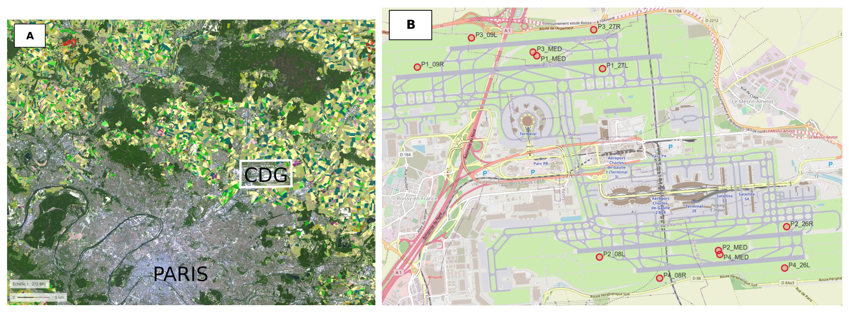For example, the financial losses for airlines for the Gandhi International Airport in India, between 2011 and 2016, reached approximately USD 3.9 million ([2]). In terms of passenger transportation, Paris Charles de Gaulle airport (Paris-CdG) is the biggest in France and the second biggest in Europe. At Paris-CdG, takeoffs and landings are reduced by a factor of two when visibility is below $600\mathrm{m}$ LVP condition (Low Visibility Procedures, for details see [3]).

Despite the improvements in numerical weather prediction (NWP) models over recent years, accurate forecasting of fog is still challenging (e.g., [3,4,5,6]). The multitude of processes involved in the fog life cycle demonstrates the complexity of this atmospheric phenomenon. It is a challenge for the NWP model to accurately represent each single process and even more so the interactions between these processes, since they exhibit numerous highly non-linear behaviour. As a consequence, fog exhibits considerable variability in space and time. Once fog has formed locally, its subsequent evolution is also of significant interest. For a site in South-East England, Price et al. (2018) [7] identified that when fog occurred, it developed into deep and optically thick fog (mature phase of fog) in approximately 50% of cases. The other 50% remained as shallow and optically thin fog (formation phase of fog) and were often inhomogeneous. NWP models must not only predict fog occurrence but also the spatial variability of fog. The hazard that a shallow local fog layer presents to airport operations is much less than that of a generalized fog layer. However, current NWP models do not accurately forecast the transition between thin and thick fogs. Accurate monitoring and timing of low-visibility situations are critical for ensuring the safety and continuity of commercial operations. It seems, therefore, important to quantify the variability of fog at local scale in both observation and NWP models.

There is abundant literature on field experiments that focuses on fog (e.g., Albany, New York [8]; Po valley, Italy [9]; Lille, France [10]; Cardington, UK [11]; Cabauw, Netherlands [12]). Field observations often suffer, however, from the local character of the measured quantities. More recently, Price et al. (2018) [7] explored the spatial variability of fog with the 3D field experiment LANFEX (The Local and Nonlocal Fog Experiment) over the UK. Furthermore, discrete observations made from meteorological towers cannot provide information about the small-scale spatial variability ($100\mathrm{m}$ to $1\mathrm{km}$) of meteorological parameters and fog [13]. For the cases with weak wind and weak turbulence, corresponding to radiation fog conditions, Cuxart et al. (2019) [14] illustrated that the small-scale variability is largest near the surface, probably linked to the terrain height and land use variability, and decreases with height. This variability is significant both thermally and dynamically. For sites less than $5\mathrm{km}$ apart such as those located in an airport area, differences can be as large as $3{\mathrm{m}\mathrm{s}}^{-1}$ or $3\mathrm{K}$ [14]. Obtaining higher-resolution observations near the surface is, therefore, particularly important in order to better understand fog evolution. Conventional in situ observations of fog are restricted to a limited number of sensors near the surface, often $100\mathrm{km}$ away. This can result in missed observations of thin fog, even if it represents more than 50% of cases ([7]).

The scale mismatch between in situ observations and gridded numerical weather prediction (NWP) forecasts is called representativeness error, and it is a challenge to be addressed when verifying forecasts. The presence of representativeness error contributes to skill estimate differences. More generally, observation errors in forecast verification have attracted more attention as the accuracy of the forecast in the short range increases. When assessing the performance of forecasts, the possibility of missed fog also proves important with the potential for false alarms to be incorrectly diagnosed when shallow fog is present but unobserved ([15]). Increased observational resolution that captures such shallow events is also not only very important for assessing forecast quality but also for the accessing the representativeness of errors needed in order to evaluate ensemble forecast ([16]).

Twelve visibility sensors are installed over the Paris-CdG airport. These allowed us to explore the small-scale spatial variability of fog and the representativeness error of visibility measurements. The Paris-CdG site, the characteristics of the visibility sensors and the data used are described in Section 2. The observed spatial variability of visibility is analysed and quantified in Section 3 through the inspection of the distribution of visibility, through the estimation of the representativeness uncertainties and through the computation of the Gini index quantifying spatial variability. To illustrate the effect of representativeness errors of local visibility observation on forecast verification, the score of a perfect forecast issued of one local observation with respect to the twelve observations of visibility made at Paris-CdG has been studied in detail in Section 3.5. Section 4 attempts to illustrate the observed heterogeneity of fog for a generalized fog event and a localized fog event. Finally, discussions and conclusions are provided in Section 5.

2. Materials and Methods

2.1. Study Area and Data

This study focuses on the Paris-CdG international airport, France (${49}^{\circ }$00${}^{\prime }$36${}^{\prime }$${}^{\prime }$ N, $2^{\circ }$32${}^{\prime }$55${}^{\prime }$${}^{\prime }$ E, mean altitude $119\mathrm{m}$). The airport is located in North-East Paris and is $23\mathrm{km}$ from the centre of the city. This geographical context means that it is under the influence of the Paris urban conurbation to the west and south and rural lands to the north and east (Figure 1A). The local topography is relatively flat with a slight eastward slope of $20\mathrm{m}$ over the airport area. Paris-CdG could be characterized by a patchwork of mostly arable fields and an urban area associated with a relatively shallow orography. Bergot et al. (2015) [17] and Bergot (2016) [18] have demonstrated with numerical LES (Large Eddy Simulation) studies that the appearances and developments of fog were significantly affected by surface heterogeneities, and this can result in heterogeneous fogs over Paris-CdG.

The airport is composed of four runways, two in the northern part and two in the southern part of the airport, divided by airport buildings and fully included in a rectangle of $7\mathrm{km}$ by $4\mathrm{km}$ oriented eastward (Figure 1B). The runways are equipped with twelve visibility sensors (forward-scattering sensor Degreane DF320 ([19]), located at both ends and in the middle of runways (see

Table 1. Strips codes and GPS coordinates of visibility sensors.

Strip Number	Strip Codes	Longitudes	Latitudes
P1	09R	2.517778	49.022136
P1	MED	2.543939	49.023765
P1	27L	2.558276	49.021920
P2	08L	2.557606	48.994861
P2	MED	2.583580	48.995802
P2	26R	2.598474	48.999213
P3	09L	2.529574	49.026325
P3	MED	2.543072	49.024290
P3	27R	2.556357	49.027490
P4	08R	2.570745	48.991832
P4	MED	2.583882	48.995240
P4	26L	2.598036	48.993290

). The visibility sensors are part of the observational operational network of the airport and are monitored by Météo-France. Both visibility sensors follow the ICAO (International Civil Aviation Organization) standards for aeronautical meteorological processes and follow the European regulation UE 2017/373 and UE 2014/139. The accuracy imposed by ICAO (ICAO annex 3A 18/11/2010) is $10\mathrm{m}$ for visibility lower than $400\mathrm{m}$, $25\mathrm{m}$ for visibility between $400\mathrm{m}$ and $800\mathrm{m}$ and 10% for visibility higher than $800\mathrm{m}$. This accuracy is very strict, and it allows obtaining state-of-the-art visibility data. These high resolution observations allow the documentation of the spatial variability of fog at the airport scale. The visibility sensors range from 0 to 60,000 m. The time resolution is one minute. The data used in this study focus on the winter season and were collected from 1 September 2017 to 30 April 2018 and 1 September 2018 to 30 April 2019.

2.2. Descriptive Statistics

2.2.1. Statistical Properties of the Dataset

The dataset consists of 828,000 lines (1440 recordings per minute per day during 575 days), and each possesses 12 visibility values, resulting in a total volume of 9,936,000 numerical values. Lines numbering 56,800 are uniformly distributed over the dataset contain at least one missing value, representing 6.86% of the total. These lines were discarded. Consequently, 93.14% of the data are available for statistical study. Despite the data quality control performed by Météo-France (following the ICAO standard), the visibility measurements from the different sensors were studied in order to detect any anomalous behavior. Firstly, all visibility measurements issued from the 12 visibility sensors were compared (marginal histogram) in Section 3.1. This allowed verifying the existence of bias between the 12 visibility sensors. Next, we focused on values below different low visibility thresholds in Section 3.2. This meant that one could detect whether or not the climatology of fog for the different visibility sensors was consistent (conditional histograms).

Then, the representativeness uncertainties were estimated by using the twelve visibility sensors in Section 3.3. To quantify the spatial variability among the visibility sensors, the Gini coefficient [20] was chosen to estimate their dispersion at each instant (Section 3.4). This index is bounded between 0 and 1, allowing comparisons between different time periods. The Gini index formula is computed as follows. Given any series of n numbers ${\left(x_i\right)}_{i\in [1:n]}$, the Gini coefficient (G) is defined as half the ratio between the mean of all differences between the series’ elements (E) and the mean of the absolute values of the series values (M).

$$\begin{array}{ccc}\hfill G& =& 0.5\frac{E}{M}\hfill \\ \hfill \mathrm{where}E& =& \frac{1}{n^2}\sum _{i=1}^n\sum _{j=1}^n\left|x_i-x_j\right|\mathrm{and}M=\frac{1}{n}\sum _{k=1}^n\left|x_k\right|\hfill \end{array}$$

(1)

Thus, in this study, $n=12$ and G are a time series $G\left(t\right)$. Originally, the Gini index was designed to confront income data within a country in order to provide a synthetic measure of wealth inequality and to make comparisons between countries. Its basic properties are as follows. Firstly, if all the $x_i$ are equal then $G=0$ because the E term is null. Secondly, if the size of the series proceeds to ∞ and if there is a maximum heterogeneity in the series (all values are equal except one), then $G\to 1$. It must be noted that a given value of G can represent many cases of dispersion. This is the price to pay for using an aggregated index. The series at a given time is assumed to be independent, with no correlation between visibility sensors. The main advantage of G is to compute a normalized coefficient making it possible to quantify the spatial variability of fog for different fog events.

Finally, the effect of spatial variability of visibility on forecast verification is studied in a perfect forecast framework in Section 3.5.

2.2.2. Definition of Low Visibility Events

At Paris-CdG international airport, adverse visibility conditions (visibility under $600\mathrm{m}$) result in the application of Low Visibility Procedures (LVP). Under these severe LVP conditions, airport take-off/landing efficiency is reduced by a factor of two, causing aircraft delays. In this context, accurate short-term forecasts of LVP conditions are considered to be a priority by airport authorities. Therefore, the $600\mathrm{m}$ threshold was studied in detail.

The dataset was used to define low visibility units (LVU): At a given time t, an LVU is defined as the number of visibility sensors that fall below the $600\mathrm{m}$ low visibility threshold (LVT). Thus, one LVU takes values between one and twelve when the entire airport is enveloped in fog. Each LVU, which is specific to a given time, represents spatial information, e.g., LVU = 3 means that 3 of the 12 visibility measurements have values under the LVT whenever they are in the airport area. There was 22,269 min of LVP conditions representing 2.69% of the entire dataset, among which only 6139 min reached the maximum value (i.e., 12) corresponding roughly to 28% of total LVP conditions (see

Table 2. LVU frequencies in minutes.

LVU	1	2	3	4	5	6	7	8	9	10	11	12	Sum
Freq (min)	3372	2166	1403	1458	1330	1713	982	929	707	800	1270	6139	22,269

for the frequencies of the LVUs values). LVU = 1, i.e., only one visibility fell below $600\mathrm{m}$, represents about 15% of the total LVP conditions. This result could be quite surprising because one would expect that it is more difficult to have 12 sensors below LVT than to have one sensor below LVT. One can explain this by the long duration of some generalized fog events.

The LVUs are not distributed at random through time. They necessarily cluster since they represent a continuous physical phenomenon. The variety of these sequences is huge (∼700), with durations ranging from a few minutes to almost a full day. The low visibility time sequences were divided into two groups. The first group is made up of sequences with at least one of its LVU at the maximum value (12) representing the fact that the entire airport is entirely covered by fog. The rationale behind this definition is that since the phenomenon is continuous in terms of time (not sporadic), the sequences would show a long continuous subsequence where fog is fully developed over the airport.

Low visibility events (LVE), as they are known, contain LVUs from 1 to 12. The studied period contains thirty-two such LVEs. When the fog is patchy (i.e., when the LVUs are low), visibility could be close to the LVT. It might happen, therefore, that no visibility crosses the LVT for a few minutes. Consequently, a small time gap of six minutes between two LVU was allowed to take into account this effect. In total, all the LVEs cover 14,271 min with 14,095 LVU (including all of the 6139 min where the fog covers the entire airport), meaning that 1.23% are time gaps. The LVE contain 63.29% of all LVUs. This result is consistent with Price et al. (2018) [7] demonstrating that 50% of fog cases developed into deep generalized fog and reached the mature phase of fog.

The second group contains all the remaining cases. They represent scattered fog, localized fog over the northern or southern side of the airport or even isolated fog. Two examples of LVU sequences defining events are shown in Figure 2. An example of generalized fog and localized fog events is presented in Section 4.

3. Results: Statistical Analysis

3.1. Statistics on Visibility

The statistical properties of the visibility measurements are studied in this section. Firstly, the statistical distribution of the visibility is presented in Figure 3 for the 12 sensors used at Paris-CdG. The shape of these distributions is very similar, with a maximum for visibility lower than $200\mathrm{m}$, followed by a minimum for visibility of around $1000\mathrm{m}$. The distribution then increases linearly until it reaches a relatively flat shape after $5\mathrm{km}$. One can observe that the maximum of the distribution corresponds to very low visibility (around $100\mathrm{m}$). However, this does not mean that visibility below $100\mathrm{m}$ is the most frequent because the time during which the visibility is less than $100\mathrm{m}$ is equal to the sum of the distribution over the interval $0–100\mathrm{m}$. To illustrate this, the visibility is below $100\mathrm{m}$ during 5820 min and between $1000\mathrm{m}$ and $5000\mathrm{m}$ during 71,527 min for P3-09L sensor. The Kolmogorov–Smirnov statistical test [21] has been applied on the 12 distributions. This test demonstrates that the distributions are identical with a confidence of more than $99.9\%$. One can conclude, therefore, that the visibility sensors are statistically homogeneous.

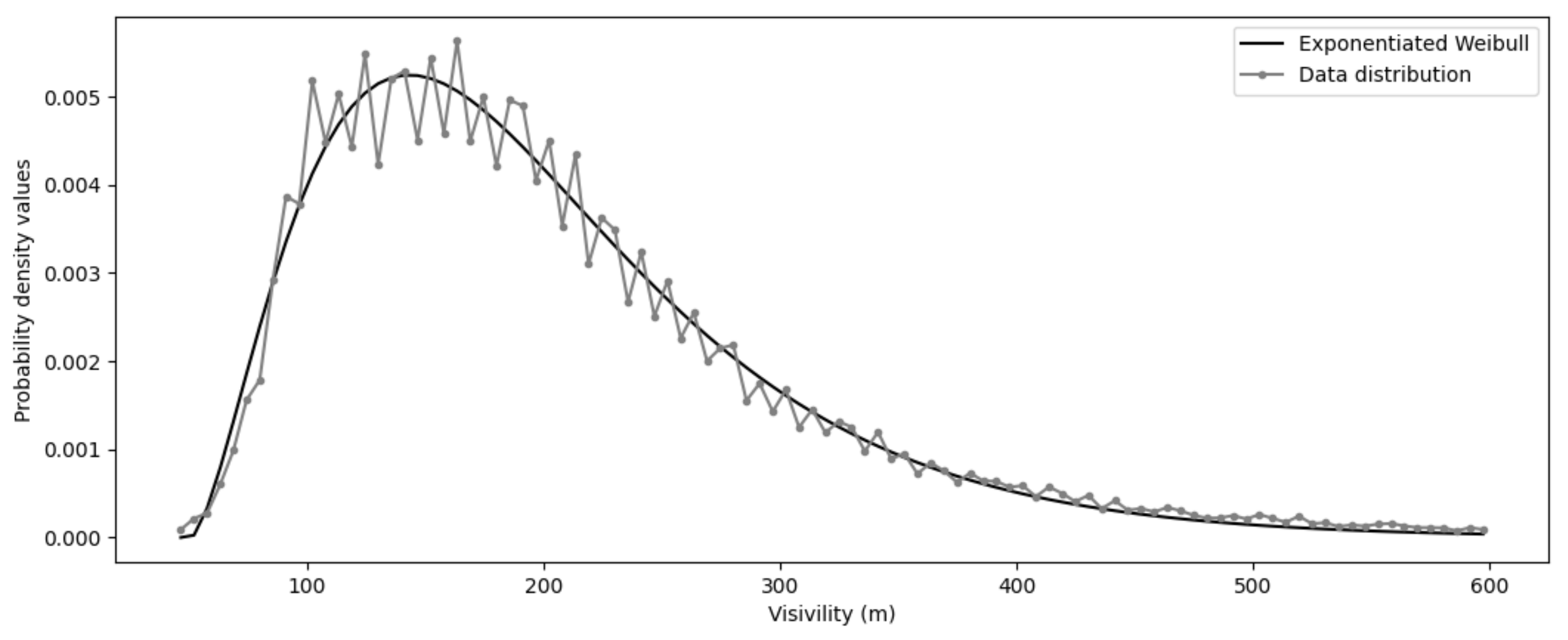
It is possible to characterize the probability density function (PDF) of visibility for the LVP events. Figure 4 shows the empirical probability density of these data along with a fit by an exponentiated Weibull probability density function. This PDF has two shape parameters (a and c) and two other parameters for location (offset of the data) and scale (dispersion of the data).

The non-linear fit provides $a=2.32$, $c=1.12$, $location=51\mathrm{m}$ and $scale=100\mathrm{m}$. Due to high temporal resolution and the total span of the dataset used in this study, it can be assumed that this characterizes the LVP events at Paris-CdG.

3.2. Conditional Statistics for Different Thresholds

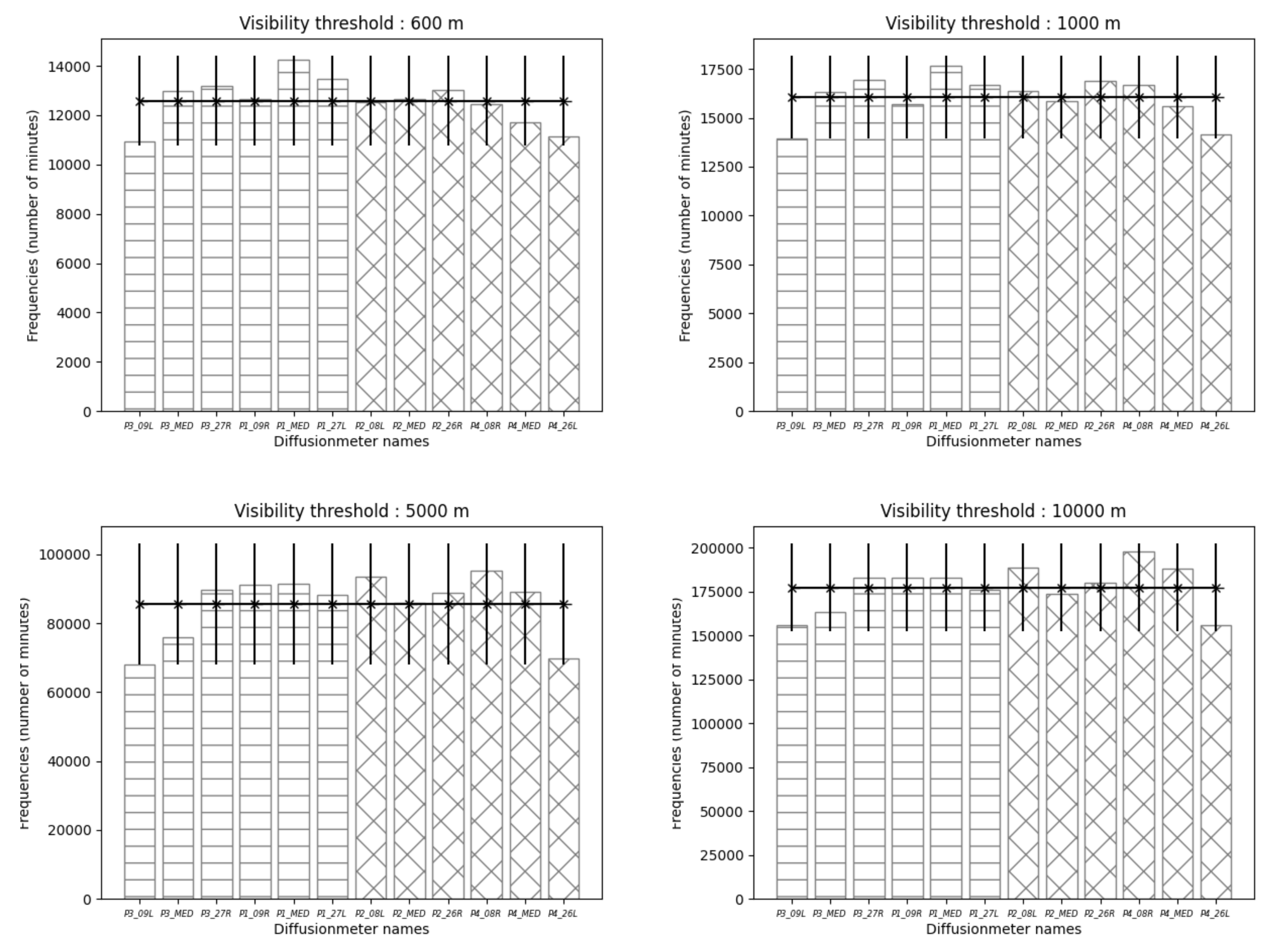
The occurrence of visibility lower than different thresholds is plotted in Figure 5 for the 12 visibility sensors. The $600\mathrm{m}$ threshold corresponds to the LVP conditions for Paris-CdG airport, $1000\mathrm{m}$ threshold corresponds to WMO fog definition and $5000\mathrm{m}$ threshold corresponds to the WMO mist definition.

The mean occurrence of LVP conditions for the 12 visibility measurements during the studied period is 12,582 min (209 h 42), with a lower mean value for the southern part of the airport (12,255 min and about 204 h 15) and upper value in the northern part (12,908 min and about 215 h 08). The maximum occurrence concerns the P1-MED sensor (237 h 34) and the minimum occurrence concerns the P3-09L sensor (182 h 04), and both are located in the northern part of the airport. It is very difficult to identify typical landscape elements to explain this spatial variability over the airport area. The standard deviation of LVP occurrence between the 12 sensors is about 15 h. The variability is slightly higher in the northern part of the airport.

The same conclusions could be drawn for the fog occurrence ($1000\mathrm{m}$ threshold), with a mean fog occurrence of 267 h 40 and a standard deviation of 17 h. The spatial variabilities for the $5000\mathrm{m}$ and 10,000 m threshold are quite similar, with mean values of 1426 h and 2955 h for 5000 m and 10,000 m thresholds, respectively. As for the LVP and fog threshold, P3-09L and P4-26L show minimal concurrence for mist.

The maximum spatial variability of the occurrence is 55 h 30 for the LVP threshold (about 26% of the mean occurrence), 61 h 16 for the fog threshold (about 23% of the mean occurrence) and 454 h 11 for the mist threshold (about 32% of the mean occurrence). Even for a relatively small homogeneous area representative of an airport area, one can observe a spatial variability of fog occurrence in the order of 25% of the mean occurrence.

3.3. Estimation of the Representativeness Uncertainties

In the current observational context, a full set of visibility data at fine scale is not commonly available. A question, therefore, arises: what is the representativeness of a given value of visibility? In other terms, given such a value, how different are all the events associated with it? In order to explore this representativeness uncertainty for low visibility, the high-density network of visibility measurements deployed at Paris-CdG is used with the following algorithm, which is described using the means, but it also holds for the minima:

1.

For an event at time t, its visibility values are $V(i,t)fori\in [1:12]$, its mean visibility over i is $m_t$ and the associated standard deviation is $s_t$;

2.

Select all t such as $m_t\le 1000\mathrm{m}$. This results in a subsample of the dataset;

3.

The subsampled mean values from 0 to 1000 are distributed in bins of fixed width. Let $Nbins$ be the number of bins and $X_b$ be the centroid location of the b-th bin;

4.

Each bin, thus characterized by $m_t$ values within its range, is associated with all the corresponding $s_t$. This results in $Nbins$ classes $C_{b}forb\in [1:Nbins]$ of standard deviations;

5.

Each class $C_b$ is characterized by the distribution $D_b$ of its elements;

6.

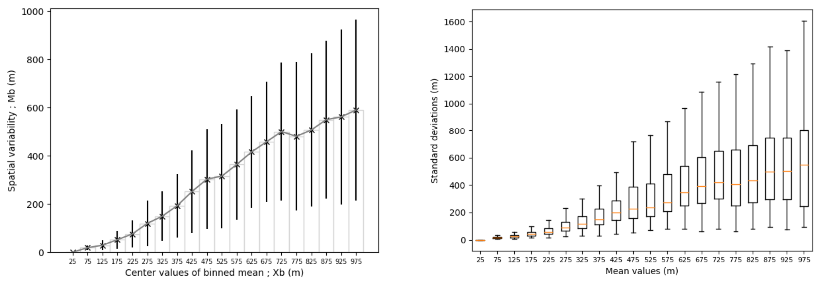
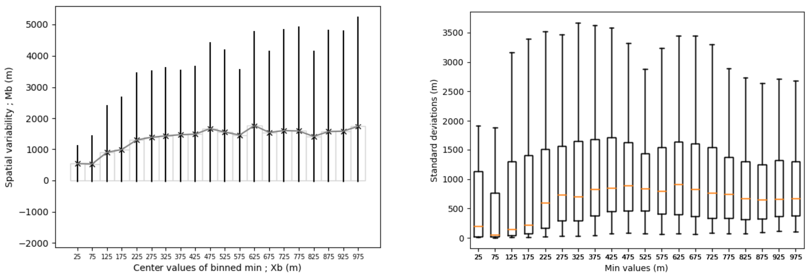
Each distribution $D_b$ is described by its mean $M_b$, its standard deviations $S_b$ and a boxplot $B{P}_b$.

$M_b$ and $S_b$ represent, respectively, the temporal mean and the temporal standard deviation of the spatial variabilities inside the class $C_b$. The curve $M_b=f\left(X_b\right)$ and the boxplots for the classes ${\left(C_b\right)}_{b\in [1:Nbins]}$ are shown, respectively, in Figure 6a,b. Figure 7 shows the same metrics as Figure 6 but for the minimum visibility values.

Except for very low visibility, it can be remarked that the mean spatial variability $M_b$ increases linearly with respect to mean visibility (Figure 6a), with a coefficient of around $0.6$. Only a few cases are in the first bin where the mean visibility is very low (lower than $100\mathrm{m}$); consequently, it is very difficult to conclude in this case. This increase in $M_b$ demonstrates a correlation between the representativeness uncertainties and the mean visibility. It seems, therefore, possible to estimate the representativeness uncertainties from the mean visibility. The inspection of the boxplots in Figure 6b reveals clearly an asymmetric distribution. If one focuses now on the mean spatial variability $M_b$ as a function of the minimum of visibility over Paris-CdG (Figure 7a), it can be noted that spatial variability is almost constant, except for minimum visibility lower than $100\mathrm{m}$. As in the previous case, the lack of data does not allow a conclusion for visibility lower than $100\mathrm{m}$. The boxplots (Figure 7b) show that all classes exhibit many outliers, indicating the local characteristics of some fog events over Paris-CdG airport. Some fog cases are a mixture of mist and LVP conditions over Paris-CdG. This point will be studied in detail in the next section. As is evident from this spatial variability analysis, the fog characteristics cannot be captured by a single visibility measurement.

One can conclude that local observations are not representative of a NWP model grid (e.g., [15]). It does not seem possible to deduce the horizontal extent of the fog layer from a local measurement, even from very low visibility measurements. It seems, therefore, very difficult to verify NWP forecast from one local visibility measurement.

3.4. Empirical Modelling of the Gini Index

The Gini index (G) defined in Equation (1) is proportional to the ratio of two terms: the mean absolute difference E and the mean value M. In order to estimate the variation of G, one builds empirical functional relationships between E and M and between G and M. This allows the approximation of the variation of G as a function of the mean visibility M. The functional fit between E and M has been calculated as follows: the E term is computed for all LVUs so that the mean visibility is less than $1000\mathrm{m}$ (black dotted curve in Figure 8a). After this, to reduce the high variability of E, a smoothing ($\widehat{E}$) of E was performed with a moving average window of which it has been empirically chosen for a value for $20\mathrm{m}$ (red curve in Figure 8a). Finally, a non-linear power law function is fitted to $\widehat{E}$ in a subset of mean values (green curve in Figure 8a), resulting in $\tilde{E}$ within this interval. Following the dataset used, it seems to be justified to use a non-linear power law function; however, it is out of the scope of this article in terms of finding the best functional fit. From this fit, it is possible to compute an empirical fitted Gini index $\tilde{G}=0.5\tilde{E}/M$ for this range of mean visibility. For very low visibilities (lower than around 100 m) characterizing very dense fogs, the dataset contains too few examples of such events; this undermines any conclusion. One can observe a growth of G with the mean visibility. For a mean visibility close to 600 m corresponding to LVP conditions, $\tilde{G}$ equals about $0.3$. For very dense fog, i.e., mean visibility close to 100 m, $\tilde{G}$ is close to $0.1$. As previously shown, this also illustrates that the spatial variability of visibility increases with respect to the mean visibility. This empirical modeling of the Gini index could be used to compare the observed spatial variability to the NWP spatial variability.

3.5. Estimation of Spatial Variability on Forecast Verification

In order to illustrate the effect of representativeness errors of local visibility observation on forecast verification, the score of a perfect forecast issued to one local observation with respect to the twelve observations of visibility made at Paris-CdG has been studied. Let us define a “perfect forecast” by one observation issued from the network of visibility measurements performed at Paris-CdG. The statistical score of this “perfect forecast” was then evaluated by considering the twelve observations of visibility. The focus here is on the LVP condition, which is the threshold mainly needed by aeronautical authorities. The statistics produced to study the quality of the LVP forecasts are based on the hit ratio (HR), the false alarm ratio (FAR), the frequency bias index (FBI), the critical success index (CSI) and the Heidke skill score (HSS). CSI is a widely used performance measure of rare events ([22]) and is commonly used to evaluated fog forecast (e.g., [23]). If a is the number of observed and forecast events (hits), b is the number of unobserved and forecast events (false alarm), c is the number of observed and unforecast events (misses) and d is the number of unobserved and unforecast events (correct rejection), these scores are defined by the following.

$$\begin{array}{ccc}\hfill HR& =& \frac{a}{a+c}\hfill \\ \hfill FAR& =& \frac{b}{a+b}\hfill \\ \hfill FBI& =& \frac{a+b}{a+c}\hfill \\ \hfill CSI& =& \frac{a}{a+b+c}\hfill \\ \hfill HSS& =& \frac{\frac{a+d}{a+b+c+d}-\frac{(a+b)(a+c)+(b+d)(c+d)}{{(a+b+c+d)}^2}}{1-\frac{(a+b)(a+c)+(b+d)(c+d)}{{(a+b+c+d)}^2}}\hfill \\ \hfill \end{array}$$

(2)

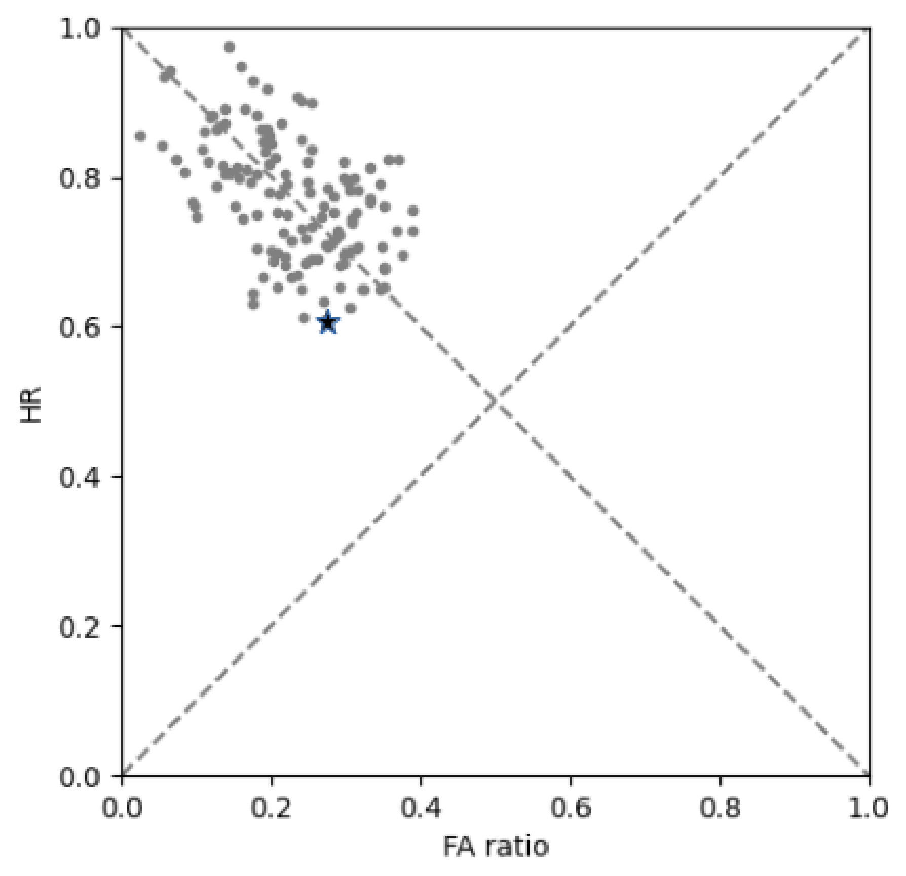
The HR is plotted against FAR in a so-called pseudo relative operating characteristic (pseudo-ROC) diagram in Figure 9. Each visibility sensor is in turn considered as the observation and tested against the others which are, therefore, considered as forecasters. This figure reveals a large dispersion of the results, with a minimum HR to the order of $0.6$ and a maximum FAR of the order of $0.4$. These values have the same magnitude as operational forecasts scores for Paris-CdG (see [24] Table 2). One can conclude that even with a perfect forecast, the score can be significantly reduced due to representativeness errors of visibility measurements. To illustrate this fact, a particular set of observation-forecasts was chosen, which contains the worst couple observation-forecast. The couple that reached this criterion was P1-09R/P4-MED (star in Figure 9). P1-09R (see Figure 1 for the location of this measurement) was, therefore, taken as the reference in the next paragraph.

First of all, the robustness of the results to the chosen threshold used to define a fog event was studied. Figure 10 shows the variation of the CSI for different thresholds. We find that the results show little dependency on the threshold for thresholds greater than about 200 m. The conclusions for LVP conditions (600 m) are, therefore, robust.

The distribution of CSI between the northern and southern part of the airport is also remarkable. The best score is for P3-09L, which is located a few hundred meters from the reference (P1-09R). The scores for the southern part of the airport are very close, around $0.4$. With the exception of P03-09L, the scores of the northern part of the airport are quite close to each other, and they are around $0.6$.

Table 3. Examples of scores for a perfect LVP forecast defined by P1-09R. See Table 1 and Figure 1 for the name and location of visibility sensors. The worst scores are shown in bold and the best scores are shown in italics.

Strip Code	TD	FAR	FBI	CSI	HSS
P3-09L	0.891	0.139	1.035	0.779	0.874
P3-MED	0.808	0.166	0.969	0.696	0.818
P3-27R	0.820	0.249	1.093	0.645	0.780
P1-09R	1	0	1	1	1
P1-MED	0.794	0.173	0.961	0.681	0.807
P1-27L	0.781	0.197	0.972	0.656	0.788
P2-08L	0.649	0.240	0.854	0.538	0.695
P2-MED	0.649	0.320	0.954	0.497	0.658
P2-26R	0.625	0.305	0.899	0.490	0.652
P4-08R	0.702	0.305	1.010	0.537	0.693
P4-MED	0.610	0.272	0.838	0.497	0.659
P4-26L	0.650	0.347	0.995	0.483	0.645

shows the scores obtained for all visibility measurements with respect to P1-09R. Once again, P3-09L located a few hundred meters from the reference had the best score, with a probability of detection of $0.89$ and a false alarm ratio of $0.14$. Even for very close measurements, the scores are not perfect, which illustrates the very small-scale variability of fog. The southern part of the airport, which is a few kilometres away from our reference, has the worst score with $0.6$ probability of detection, $0.3$ false alarm ratio, $0.48$ CSI and $0.64$ HSS.

The HSS score is positive for all verification pairs, which means that the “forecasts” provided by the other visibility measurements are all better than the random forecast. It demonstrates that the variability is not purely random.

One can conclude that when only one station is considered to evaluate forecast, the results may fluctuate depending on the particular chosen station. To overcome this problem, the verification should take into account the representativeness of observation, although this is frequently overlooked. It is important to emphasize that no single measure can adequately describe forecast errors (e.g., [16]).

4. Results: Case Study

This section is devoted to the presentation of various low visibility events encountered at Paris-CdG airport during the studied period.

The criterion used to select fog events, i.e., at least one measurement unit of Paris-CdG is under the low visibility threshold-LVT-(600 m), has detected a large amount of contiguous low visibility events (in total 686); however, only $23\%$ last for more than 10 min, $8.7\%$ more than 30 min and $5\%$ for more than an hour. The analysis of every case has allowed classing those events into two main types: the events containing at least one instant with all twelve visibilities below the low visibility threshold (thirty-two events) and the rest. The first group contains mainly deep fog events, whilst the second contains localized fogs, especially cases where only the north or the south of the airport is caught up in the fog. In the following subsections, theses cases will be known as “generalized events” and “localized fog events”, respectively. These low visibility events can occur at any time during the day. Nevertheless, the burden caused by their occurrence is greater during some phases of the day (especially the morning hub). This provides a criterion with which to select events.

4.1. Generalized Fog Events

As previously stated, this group of events is defined by the fact that low visibility was generalized over Paris-CdG airport. This means that the twelve visibilities are below the visibility threshold at least once. Naturally, it is expected that it holds longer because the phenomena is continuous and because the underlying physics are steady for a while, resulting in stationary situations.

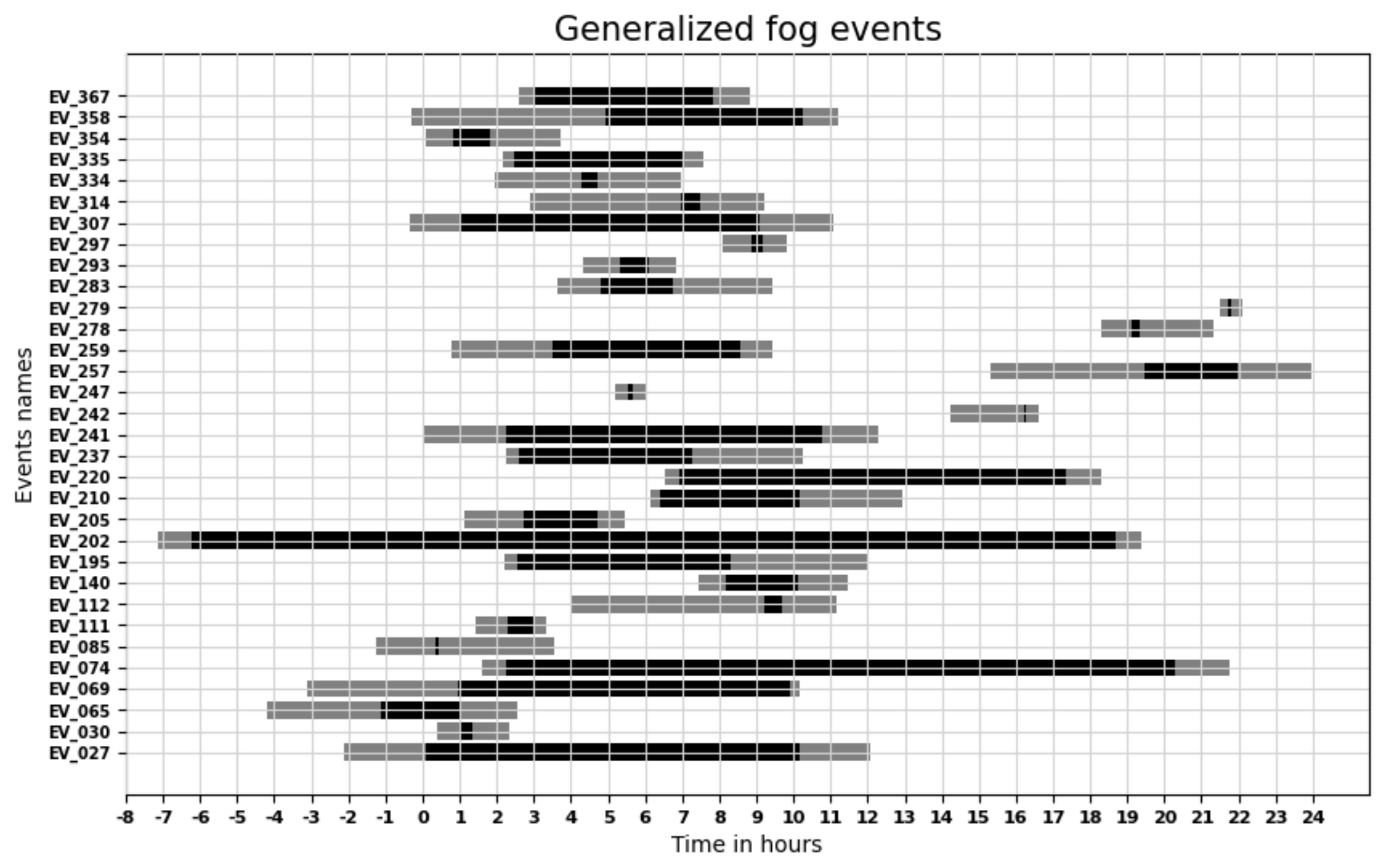
Figure 11 shows the complete set of “generalized events”. On the time axis (UTC), negative time values indicate that the events start on the previous day. The black bars indicates the mature phases of the events and before and after their formation and dissipation phases. The mature phase of fog event is defined by the time when all twelve visibility measurements are below LVT.

One can observe great variability of generalized cases events. Some events are very short whilst others last for more than a day. The duration of the formation and dissipation phases is also very different. The formation phase lasts from 14 min and 314 min. The mean duration of the formation phase is about 1h 30 (98 min). The dissipation phase may also be very short (15 min) or very long (222 min) for a mean value of about 86 min. In Section 2, Figure 2 shows examples of temporal profiles of events, i.e., the evolutions through time of the number of forward-scattering sensors under the low visibility threshold. Examining such kinds of profiles for this class of events allows them to be grouped into three subgroups:

1.

The events with a long sequence that are sometimes not fully continuous during which the airport is caught by a deep fog. Some of these events lasts more than 12 hours. These are EV_027, EV_069, EV_074, EV_195, EV_202, EV_210, EV_220, EV_237, EV_241, EV_259, EV_283, EV_307, EV_335, EV_358 and EV_367. All of them include sunrise in their evolution.

2.

The events EV_065, EV_085, EV_140, EV_205, EV_257, EV_314, EV_334 and EV_354. They are generally shorter, and the northern side and southern side of the airport are much less phased.

3.

All the other events, which should have been included in the “atypical fog event” group.

As an example of long generalized fog event, EV_195 has been chosen. This event took place from 02:12UTC to 12:00UTC on 15 November 2018 and lasted almost ten hours. After a short formation phase (20 min) that began first in the southern part of the airport, a mature phase of almost six hours took place. The event ended with a dissipation phase lasting almost four hours where the northern side remained more active than the southern one. All the information about this event is summed up in Figure 12. Figure 12a shows the time series of the minimum among all visibility sensors, which is the deepest visibility trajectory for this event. When added to this curve, the coloured dots indicate the number of sensors under the low visibility threshold (LVT). The vertical red line marks the sunrise. Figure 12b shows the times series of LVU for the entire airport and the northern and southern parts.

Northern and southern time series are individual so as to show the two different dynamics over the two sides of the airport. The fog forms firstly in the southern part of the airport and generalizes rapidly to encompass the entire airport. The formation phase is very short, which is around 20 min. Figure 12c shows the time series of Gini indexes G which quantifies the variability between the visibility time series. During the formation phase, G is relatively strong around $0.6$, reflecting high variability. The mature phase lasts around 350 min. During the mature phase, G is roughly constant and remains around $0.1$. This value corresponds to the mean Gini index $\tilde{G}$ estimated in Figure 8b for very dense fog. After sunrise, G shows more variability and one can observe the appearance of waves at a frequency of about 60 min. The dissipation phase is very long and is around 220 min. The fog dissipates first of all in the southern part of the airport but remains dense in the northern part. During this dissipation phase, the fog displays strong variability over the airport, some runways being in LVP conditions and others are not. One can observe that for this event, G summarizes the spatial variability of fog during the entire life cycle well.

4.2. Localized Fog Events

The duration of this class of localized fog events ranges from one minute to five hours. Many of them show only a few measurements under the low visibility threshold; hence, it was decided to concatenate the events according to the time length of the void between them. It reduces their number and takes into account some kind of instability close to the threshold value. To perform this, the delays between the events were computed, and then, for a wide range of glueing time length, two events were concatenated if the void between them was smaller than the given gluing time length.

A 45 min delay was chosen, and 180 events were retained as valid. It was also found that they showed strong spatial and temporal variability. Events for which only one side of the airport is caught by the fog can be remarked.

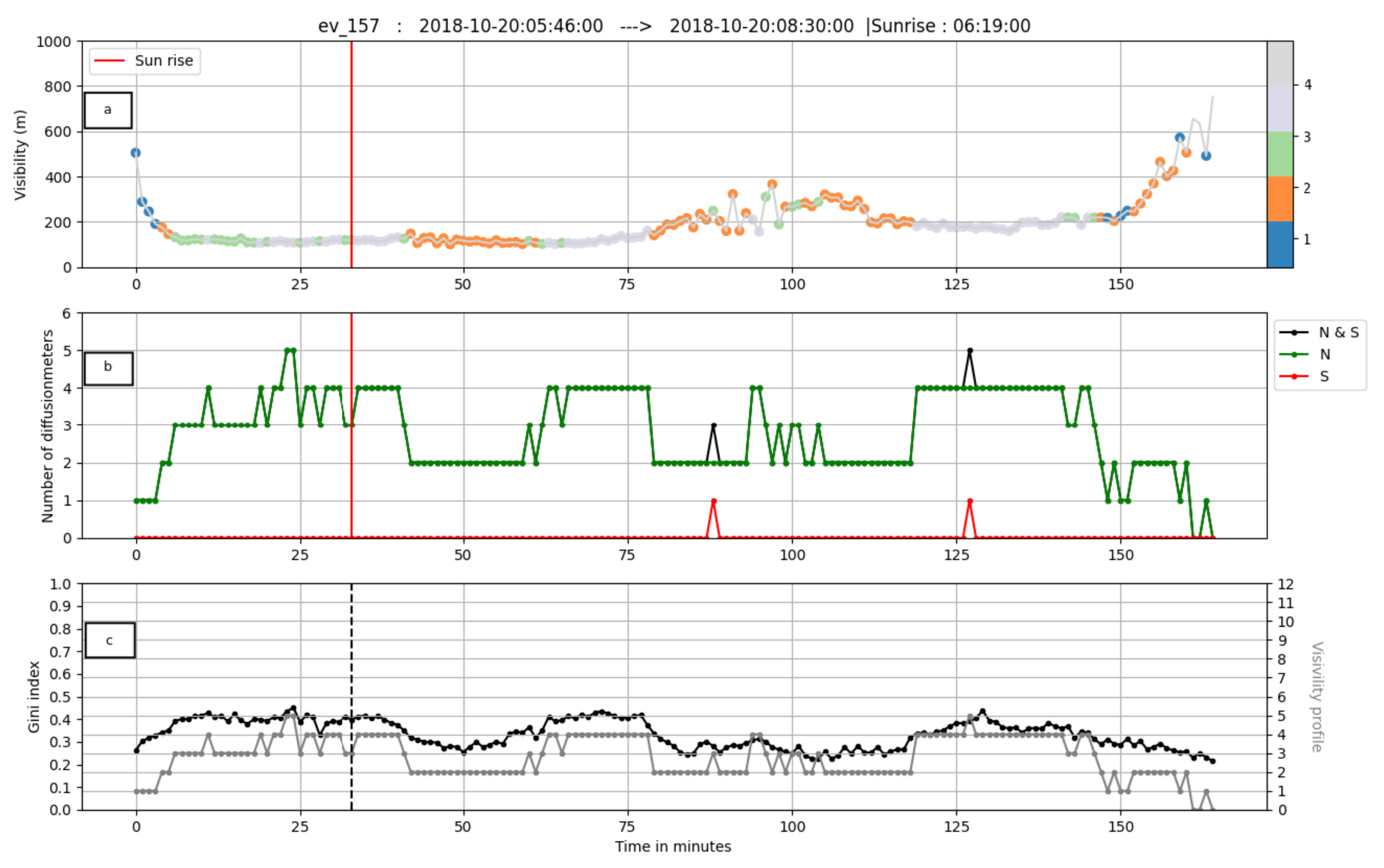
Figure 13 shows one example of localised events. This event started approximately 30 min before sunrise on 20 October 2018 at 05:46UTC and lasted for 164 min. In this example, the event occurred during the early morning departure time, the fog was in the northern part of the airport and the number of LVU was fluctuating. Nevertheless the minimum visibility trajectory shows very low values, as low as in Figure 12a. From a forecasting point of view, it seems hard to decide if the event, once started, will keep on going. G was around $0.3$ and showed oscillations with a period around 45 min. This value is characteristic of fog with a mean visibility close to 600 m (LVT), see Figure 8b.

5. Discussion and Conclusions

The main goal of this work was to explore the small-scale variability of fog over the Paris-CdG airport area. The twelve visibility measurements installed at Paris-CdG allowed the estimation of spatial variability of visibility at sub-kilometre horizontal scale. This work is certainly a pioneering attempt to quantify the variability of fog at the local scale.

The variability inside the sub-kilometre area is significant for fog, whatever the studied fog characteristics. When focusing at the local-scale to an order of $100\mathrm{m}{}^{-1}$ km, this study has demonstrated that the standard deviation of low visibility is of the same order as the mean visibility, indicating the importance of local scale in the evolution of fog events. This study indicated that when using visibility measurements, one point of measurement may be far from the representativeness of the sub-kilometre scale area and can create problems if used for verifying or initializing numerical models. This work demonstrated that the fog characteristics cannot be captured by a local measurement of visibility. It also appears that it is impossible to deduce fog extension at local scale from a local measurement, even for low visibility such as LVP cases. The existence of such heterogeneities in visibility indicates that local processes, at a $100\mathrm{m}$ to $1\mathrm{km}$ scale, drive the life cycle of fog, particularly during the formation and dissipation phase. This illustrates that for a scale of the order of hectometre, the circulation generated, for example, by surface heterogeneities may be of particular importance and could explain the difficulty of the current NWP in correctly simulating the fog.

The lack of representativeness of a measurement network is a sensitive problem in many aspects of meteorology, such as weather modelling, assimilation and verification. It is, however, especially crucial in physical fields such as fog which is highly discontinuous in space and time or in regions where data availability is scarce. The results and conclusions obtained in a verification process can be strongly influenced by the verification methodology, especially when some assumptions are made in order to avoid the limitations of the observational data (i.e., the lack of representativeness of the data or poor area coverage). The representativeness error of visibility clearly follows an asymmetric distribution. It also seems impossible to deduce fog extension at a kilometre scale from a local measurement, even for low visibility such as LVP cases. This study showed that observation of mean visibility would be more useful for verifying forecasts than local-scale observation. When the spatial representativeness of the observational data is incomplete, significant biases may be introduced in the calculated scores and results. Note that when only one station is considered, the results could fluctuate depending on the particular chosen station. To overcome this problem, the forecasts verification should take into account the representativeness error of visibility, and one can emphasize that the forecast error cannot be adequately described with one single local observation. This work demonstrated that a large dispersion of forecast quality could be obtained when using one observation at a local-scale due to representativeness errors of visibility measurements. This dispersion has the same order of magnitude as the current NWP forecast quality of fog.

An attempt to quantify the scale heterogeneity of fog was made using the Gini index. Initially, the Gini index was designed to provide a synthetic measure of wealth inequality and to make comparisons between countries. It was used in this study to provide a synthetic measure of visibility heterogeneity. The Gini index could be computed easily from a network of visibility measurements to estimate the variability of visibility over an area, such as that of an airport. Case studies of generalized and local fog events illustrated that the Gini index summarizes the fog variability well during the entire life cycle of fog. This index has allowed highlighting the appearance of waves during the dissipation phase of fog. Furthermore, understanding how and why a shallow fog layer transitions to a deep layer is essential. The use of Gini index at Paris-CdG has showed that shallow fog layers can exist long before evolution and even in the absence of a deeper fog layer.

Observations remain a key point for the improvement of fog forecasting by providing new insights into fog behaviour. Observations, however, were not often capable of documenting all of the processes affecting fog due to their local nature. The dynamics of a fog layer is very subtle, and it seems impossible to deduce all the aspects of these dynamics with local measurements issued for ground sensors, tower or vertical soundings. Both LES simulations (e.g., [25]) and specific observations (e.g., [26]) showed the presence of waves driving the fog life cycle. The effects of these waves on standard local measurements could not be distinguished from typical variations inside the stable boundary layer. Price and Stokkereit (2020) [26] have illustrated that a shallow stable layer of fog could be strongly influenced by the passage of gravity waves; therefore, standard local measurements were not representative of the general wider scale conditions. Consequently, many important processes occurring in fog do not produce conclusive signals in standard meteorological measurements. High density visibility data, such as in Paris-CdG, illustrate well the inhomogeneous nature of fog, particularly for fog microphysical properties. Since the present study focus on only one site (Paris-CdG), it would be fine to generalize this kind of study for international airports where several visibility sensors are available. Significant variability has already been observed in the droplet size distribution in fog [27]. One can, therefore, wonder about the representativeness of microphysical measurements at the local scale, e.g., during fog field experiments.

The subgrid variability of fog microphysical properties is also very important for NWP models. Representing subgrid variability in microphysical parameters can have a high impact on radiation fields. It is clear from this study that there is a local scale variability in visibility and, consequently, in the fog microphysical properties. It seems necessary to quantify the subgrid variability of fog properties and to estimate the PDF of fog properties. Correcting physical parametrization of NWP is of great interest. There is a great deal of variability in the observed microphysical properties of fog, and NWP microphysical parameterizations should be adjusted to draw the PDF of microphysical properties for utilisation in stochastic physics schemes for ensemble forecasts.