
Characterization of PM10 Emission Rates from Roadways in a Metropolitan Area Using the SCAMPER Mobile Monitoring Approach

Abstract
:1. Introduction
- E = Particulate matter emission rate in the units of g/VKT
- k = A constant dependent on the aerodynamic size range of PM (0.62 for PM10)
- sL = Road surface silt loading of material smaller than 75 μm in g m−2
- W = mean vehicle weight in U.S. tons
- VKT = vehicle kilometer traveled
- Provide actual measurements of PM10 emission rates from roadways that could be used to construct a data-based emission inventory.
- Evaluate the significance of construction activities on PM10 emission rates.
- Determine if there are seasonal changes in the emission rates.
- Evaluate the precision of the measured emission rates.
2. Materials and Methods
2.1. Test Route
- I: Less than 10,000 ADT: 43 km total
- II: 10,000–19,999 ADT: 48 km total
- III: 20,000–29,000 ADT: 12 km total
- IV: Greater than 30,000 ADT: 7 km total
- Limited Access: 70 km total
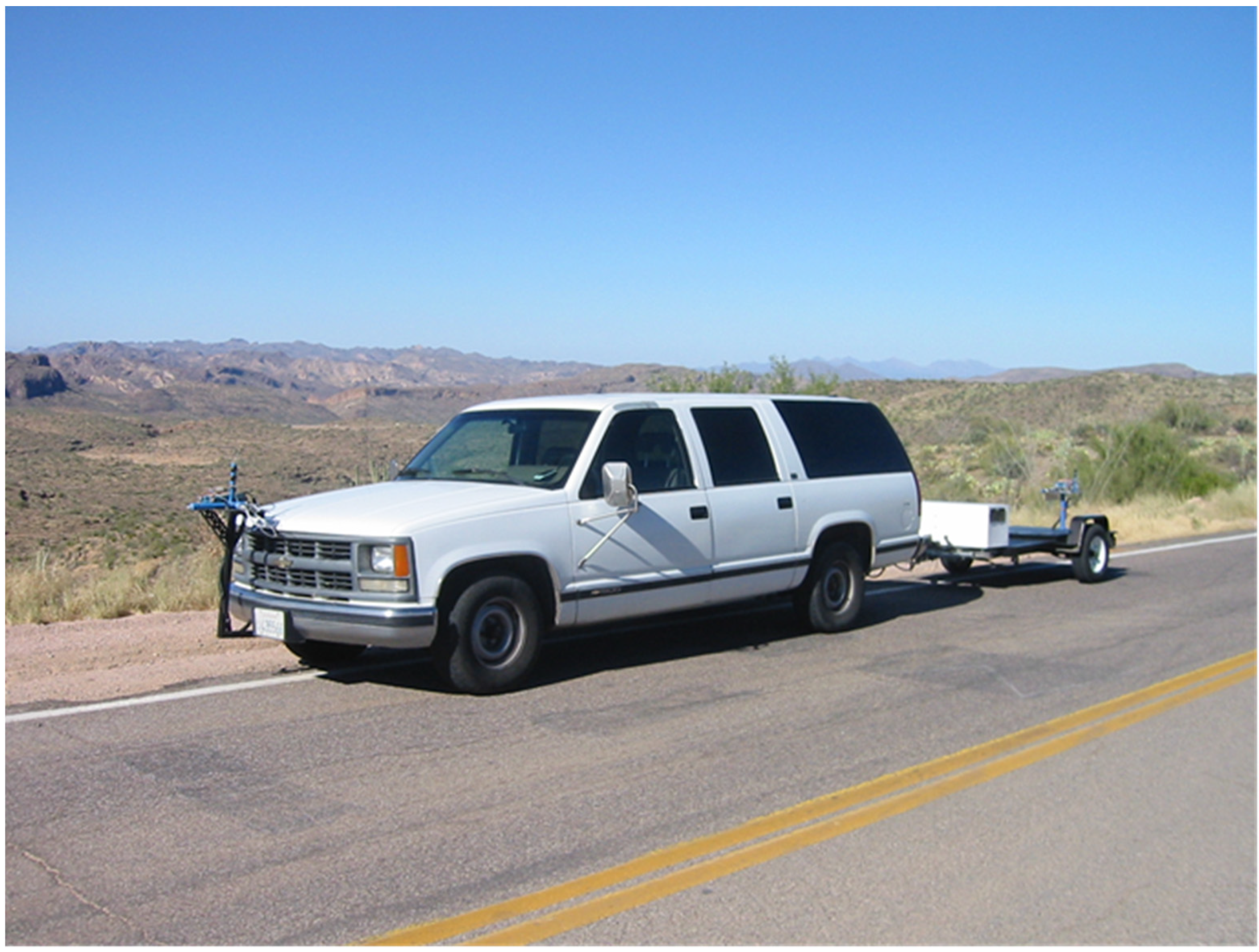
2.2. SCAMPER Description
2.3. Data Quality Control and Quality Assurance
3. Results
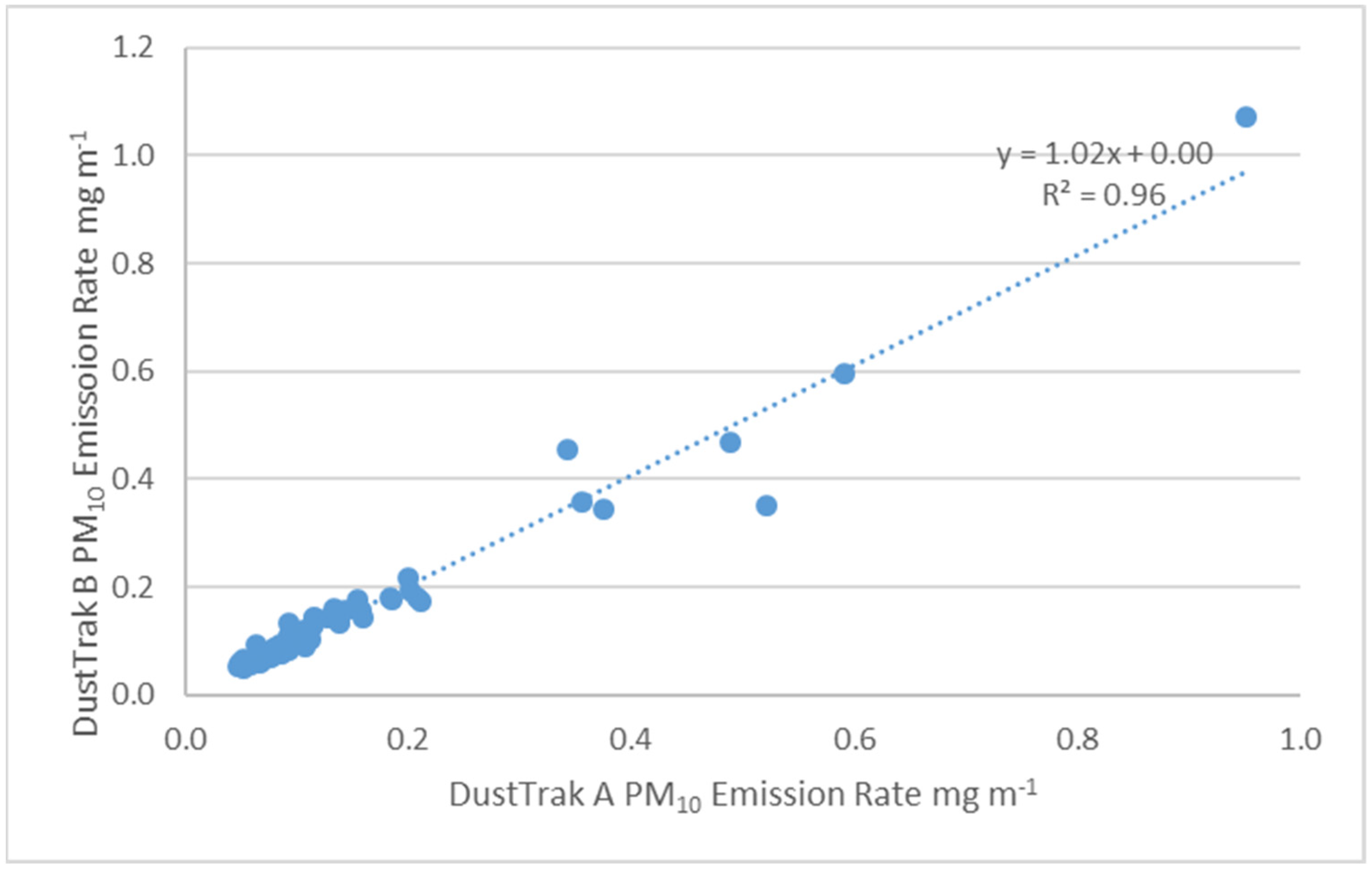
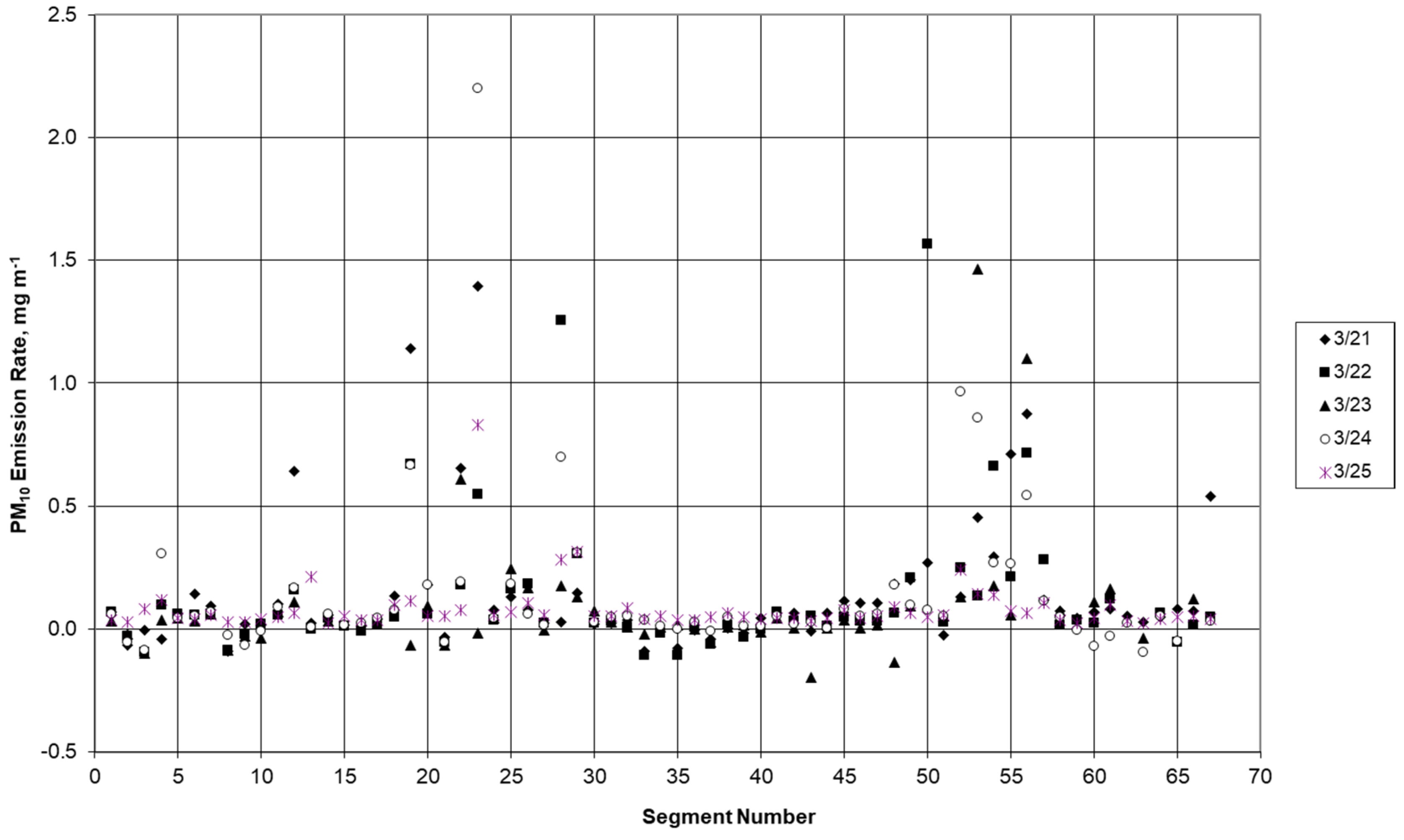
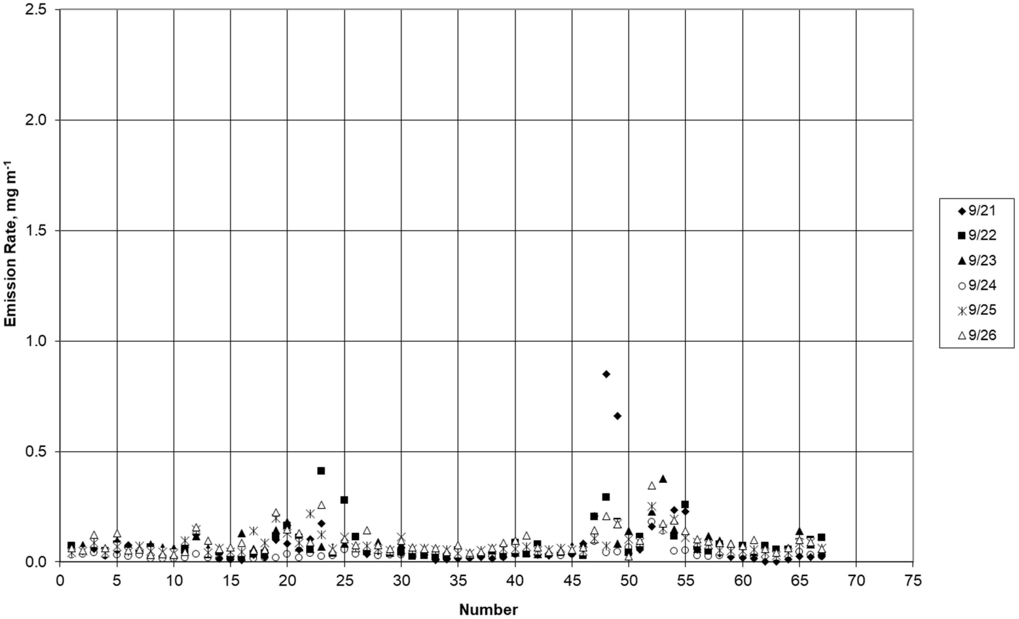
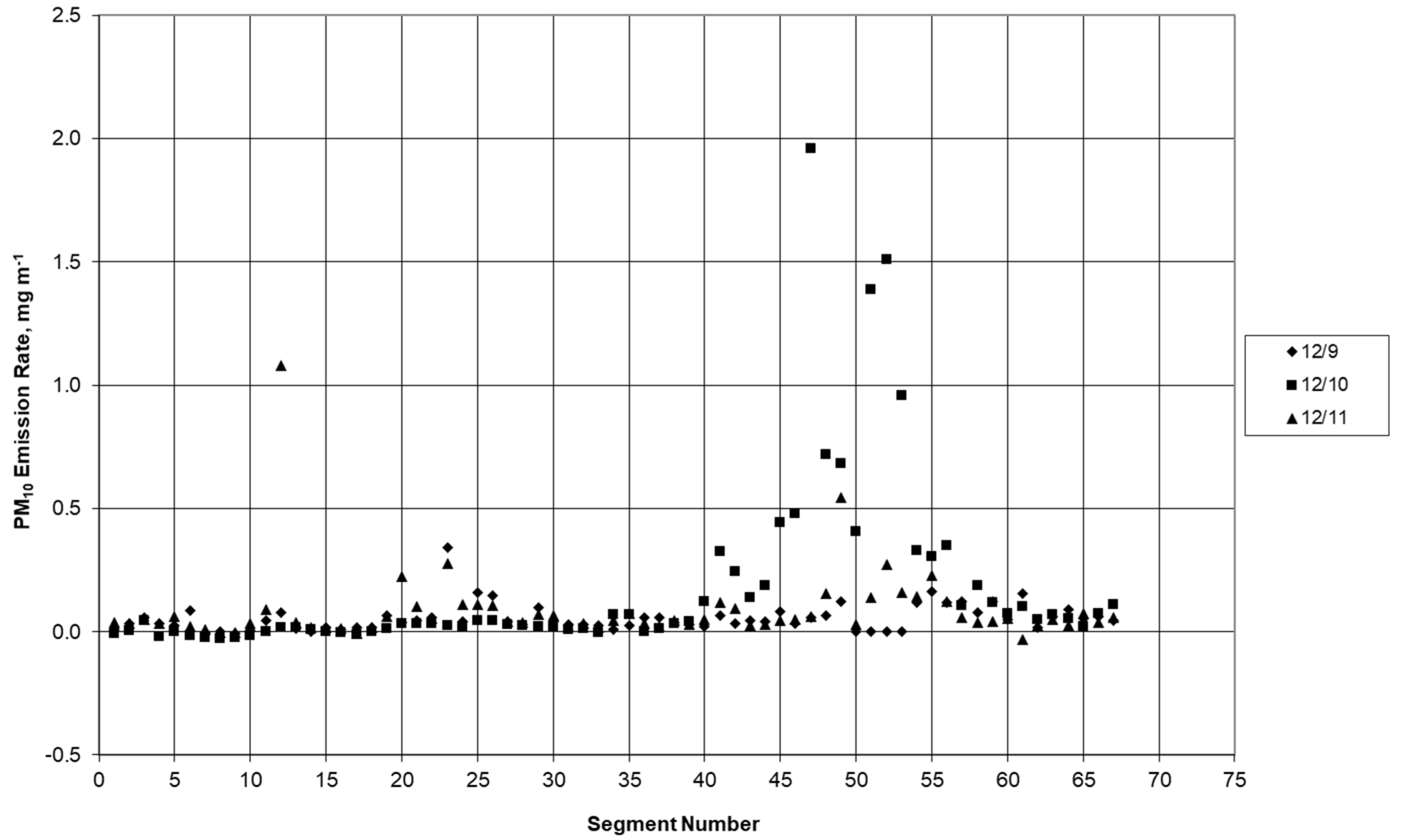
3.1. Precision Test Loop
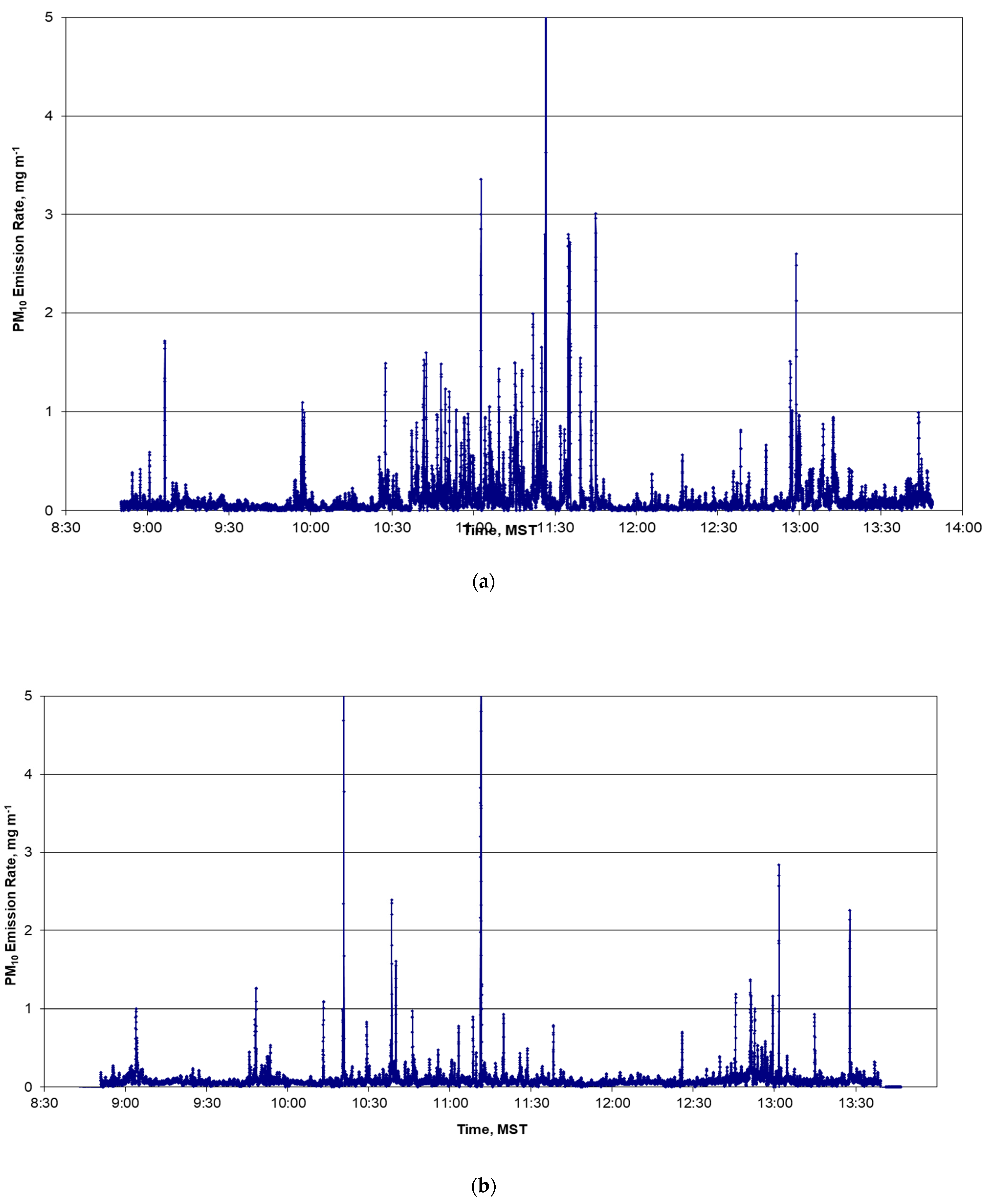
3.2. Summary of Emission Rate Data
3.3. Comparison of DustTrak PM10 with Filter Samples
4. Discussion and Conclusions
Author Contributions
Funding
Institutional Review Board Statement
Informed Consent Statement
Data Availability Statement
Acknowledgments
Conflicts of Interest
References
- Pope, C.A.; Thun, M.J.; Namboodiri, M.M.; Dockery, D.W.; Evans, J.S.; Speizer, F.E.; Heath, C.W. Particulate Air Pollution as a Predictor of Mortality in a Prospective Study of U.S. Adults. Am. J. Respir. Crit. Care Med. 1995, 151, 669–674. [Google Scholar] [CrossRef]
- Chow, J.C.; Watson, J.G.; Lowenthal, D.H.; Solomon, P.A.; Magliano, K.; Ziman, S.; Richards, L.W. PM10 Source Apportionment in California’s San Joaquin Valley. Atmos. Environ. 1992, 26A, 3335–3354. [Google Scholar] [CrossRef]
- Harrison, R.H.; Stedman, J.; Derwent, D. New Directions: Why are PM10 concentrations in Europe not falling? Atmospheric science perspectives special series. Atmos. Environ. 2008, 42, 603–606. [Google Scholar] [CrossRef]
- Amato, F.; Pandolfi, M.; Escrig, A.; Querol, X.; Alastuey, A.; Pey, J.; Perez, N.; Hopke, P.K. Quantifying road dust resuspension in urban environment by Multilinear Engine: A comparison with PMF2. Atmos. Environ. 2009, 43, 2770–2780. [Google Scholar] [CrossRef]
- Venkatram, A.; Fitz, D.; Bumiller, K.; Du, S.; Boeck, M.; Ganguly, C. Using a dispersion model to estimate emission rates of particulate matter from paved roads. Atmos. Environ. 1999, 33, 1093–1102. [Google Scholar] [CrossRef]
- Kauhaniemi, M.; Kukkonen, J.; Härkönen, J.; Nikmo, J.; Kangas, L.; Omstedt, G.; Ketzel, M.; Kousa, A.; Haakana, M.; Karppinen, A. Evaluation of a road dust suspension model for predicting the concentrations of PM10 in a street canyon. Atmos. Environ. 2011, 45, 3646–3654. [Google Scholar] [CrossRef]
- Denby, B.; Sundvor, I.; Johansson, C.; Pirjola, L.; Ketzel, M.; Norman, M.; Kupiainen, K.; Gustafsson, M.; Blomqvist, G.; Omstedt, G. A coupled road dust and surface moisture model to predict non-exhaust road traffic induced particle emissions (NORTRIP). Part 1: Road dust loading and suspension modelling. Atmos. Environ. 2013, 77, 283–300. [Google Scholar] [CrossRef]
- Abu-Allaban, M.; Gillies, J.A.; Gertler, A.W. Application of a multi-lag regression approach to determine on-road PM10 and PM2.5 emission rates. Atmos. Environ. 2003, 37, 5157–5164. [Google Scholar] [CrossRef]
- Abu-Allaban, M.; Gillies, J.A.; Gertler, A.W.; Clayton, R.; Proffitt, D. Tailpipe, resuspended road dust, and brake-wear emission factors from on-road vehicles. Atmos. Environ. 2003, 37, 5283–5293. [Google Scholar] [CrossRef]
- Kumar, A.V.; Patil, R.; Nambi, K. A composite receptor and dispersion model approach for estimation of effective emission factors for vehicles. Atmos. Environ. 2004, 38, 7065–7072. [Google Scholar] [CrossRef]
- Claiborn, C.; Mitra, A.; Adams, G.; Bamesberger, L.; Allwine, G.; Kantamaneni, R.; Lamb, B.; Westberg, H. Evaluation of PM10 emission rates from paved and unpaved roads using tracer techniques. Atmos. Environ. 1995, 29, 1075–1089. [Google Scholar] [CrossRef]
- Kantamaneni, R.; Adams, G.; Bamesberger, L.; Allwine, E.; Westberg, H.; Lamb, B.; Claiborn, C. The measurement of roadway PM10 emission rates using atmospheric tracer ratio techniques. Atmos. Environ. 1996, 30, 4209–4223. [Google Scholar] [CrossRef]
- Ferm, M.; Sjöberg, K. Concentrations and emission factors for PM2.5 and PM10 from road traffic in Sweden. Atmos. Environ. 2015, 119, 211–219. [Google Scholar] [CrossRef]
- Sehmel, G. Particle resuspension from an asphalt road caused by car and truck traffic. Atmos. Environ. 1973, 7, 291–309. [Google Scholar] [CrossRef]
- Cowherd, C., Jr.; Englehart, P.J. Paved Road Particulate Emissions; U.S. Environmental Protection Agency Document EPA-600/7-84-077; U.S. Environmental Protection Agency: Washington, DC, USA, 1984. [Google Scholar]
- Xueli, J.; Dahe, J.; Simei, F.; Hui, Y.; Pinjing, H.; Boming, Y.; Zhongliang, L.; Chang, F. Road dust emission inventory for the metropolitan area of Shanghai City. Atmos. Environ. Part A Gen. Top. 1993, 27, 1735–1741. [Google Scholar] [CrossRef]
- Veranth, J.M.; Pardyjak, E.R.; Seshadri, G. Vehicle-generated fugitive dust transport: Analytic models and field study. Atmos. Environ. 2003, 37, 2295–2303. [Google Scholar] [CrossRef]
- U.S. Environmental Protection Agency. AP-42 Compilation of Air Emission Factors, Section 13-2.1 Paved Roads, January 2011. Available online: https://www.epa.gov/sites/default/files/2020-10/documents/emission_factor_documentation_for_ap-42_section_13.2.1_paved_roads_.pdf (accessed on 20 September 2021).
- Kuhns, H.; Etyemezian, V.; Landwehr, D.; MacDougall, C.; Pitchford, M.; Green, M. Testing re-entrained aerosol kinetic emissions from roads (TRAKER): A new approach to infer silt loading on roadways. Atmos. Environ. 2001, 35, 2815–2825. [Google Scholar] [CrossRef]
- Pirjola, L.; Johansson, C.; Kupiainen, K.; Stojiljkovic, A.; Karlsson, H.; Hussein, T. Road Dust Emissions from Paved Roads Measured Using Different Mobile Systems. J. Air Waste Manag. Assoc. 2010, 60, 1422–1433. [Google Scholar] [CrossRef] [Green Version]
- Mathissen, M.; Scheer, V.; Kirchner, U.; Vogt, R.; Benter, T. Non-exhaust PM emission measurements of a light duty vehicle with a mobile trailer. Atmos. Environ. 2012, 59, 232–242. [Google Scholar] [CrossRef]
- Fitz, D.R.; Bumiller, K.; Bufalino, C.; James, D.E. Real-time PM10 emission rates from paved roads by measurement of concentrations in the vehicle’s wake using on-board sensors. Part 1. SCAMPER method characterization. Atmos. Environ. 2020, 230, 117483. [Google Scholar] [CrossRef]
- Fitz, D.R.; Bumiller, K.; Etyemesian, V.; Kuhns, H.D.; Gillies, J.A.; Nikolich, G.; James, D.E.; Langston, R.; Merle, R.S., Jr. Real-time PM10 emission rates from paved roads by measurement of concentrations in the vehicle’s wake using on-board sensors. Part 2. Comparison of SCAMPER, TRAKER™, flux measurements, and AP-42 silt sampling under controlled conditions. Atmos. Environ. 2021, 256, 118453. [Google Scholar] [CrossRef]
- Nicholson, K.W.; Branson, J.R.; Giess, P.; Cannell, R.J. The effects of vehicle activity on particle resuspension. J. Aerosol Sci. 1989, 20, 1425–1428. [Google Scholar] [CrossRef]


| Length | Vol | # of | Predominant | ||||||
|---|---|---|---|---|---|---|---|---|---|
| Seg # | Intersection | On Street | Dir | km | From Street | To Street | Class | Lanes | Land Use |
| Begin: 1st Ave/Van Buren | 1st Ave | SB | --- | II | 3 | Commercial | |||
| 1 | 1st Ave/Van Buren | Van Buren St | EB | 3.2 | 1st Ave | 20th St | II | 2 | Commercial |
| 2 | Van Buren/20th St | 20th St | NB | 0.8 | Van Buren St | Roosevelt St | III | 5 | Mixed |
| 3 | 20th St/Roosevelt St | Roosevelt St | WB | 2.4 | 20th St | 7th St | I | 1 | Residential |
| 4 | Roosevelt/7th St | 7th St | NB | 0.8 | Roosevelt | I-10E on-ramp | IV | 3 | Mixed |
| 5 | I-10 East/7th St | I-10 East | EB | 1.6 | 7th St | SR 202 | Fwy | Mixed | |
| 6 | I-10 East/SR 202 | SR 202 | EB | 14.4 | SR 202 | SR 101 | Fwy | Mixed | |
| 7 | SR 202/SR 101 | SR 101 | NB | 2.4 | SR 202 | Thomas Rd | Fwy | Agricultural | |
| 8 | SR 101/Thomas Rd | Thomas Rd | WB | 3.2 | SR 101 | Scottsdale Rd | IV | 2 | Residential |
| 9 | Thomas/Scottsdale Rd | Scottsdale Rd | SB | 3.2 | Thomas Rd | McKellips Rd | IV | 3 | Comm/Res |
| 10 | Scottsdale/McKellips Rd | McKellips Rd | EB | 6.7 | Scottsdale Rd | Alma School Rd | II | 2 | Agricultural |
| 11 | McKellips/Alma School | Alma School Rd | SB | 2.9 | McKellips Rd | 8th St | II | 3 | Industrial |
| 12 | Alma School Rd | SB | 4.8 | 8th St | US 60 | III | 3 | Commercial | |
| 13 | Alma School/US 60 | US 60 | EB | 12.6 | Alma School Rd | Higley Rd | Fwy | Mixed | |
| 14 | US 60/Higley | Higley Rd | SB | 2.4 | US 60 | Guadalupe Rd | II | 3 | Agricultural/Res |
| 15 | Higley Rd | SB | 1.6 | Guadalupe Rd | Elliot Rd | II | 3 | Agricultural/Res | |
| 16 | Higley Rd | SB | 1.6 | Elliot Rd | Warner Rd | II | 1 | Agricultural/Res | |
| 17 | Higley Rd | SB | 1.6 | Warner Rd | Ray Rd | II | 1 | Agricultural/Res | |
| 18 | Higley Rd | SB | 1.6 | Ray Rd | Williams Field Rd | II | 1 | Agricultural/Res | |
| Inner Loop #1 | |||||||||
| 19 | Higley/Williams Field Rd | Williams Field Rd | WB | 2.4 | Higley Rd | Santan Valley Pky | I | 1 | Agricultural/Res |
| 20 | Williams Field/Santan Valley | Santan Valley Pky | NB | 1.8 | Williams Field Rd | Ray Rd | I | 1 | Agricultural/Res |
| 21 | Santan Valley/Ray Rd | Ray Rd | EB | 2.4 | Santan Valley Pky | Higley Rd | I | 1 | Agricultural/Res |
| 18 | Ray Rd/Higley Rd | Highley Rd | SB | 1.6 | Ray Rd | Williams Field Rd | I | 1 | Agricultural/Res |
| 22 | Higley Rd | SB | 1.6 | Williams Field Rd | Pecos Rd | I | 1 | Agricultural/Res | |
| 23 | Higley/Pecos Rd | Pecos Rd | WB | 1.6 | Higley Rd | Greenfield Rd | I | 3 | Agricultural/Res |
| 24 | Pecos Rd | WB | 1.8 | Greenfield Rd | Val Vista Rd | I | 3 | Agricultural/Res | |
| 25 | Pecos Rd | WB | 1.8 | Val Vista Rd | Lindsay Rd | I | 2 | Agricultural/Res | |
| 26 | Pecos Rd | WB | 1.4 | Lindsay Rd | Gilbert Rd | I | 1 | Agricultural/Res | |
| 27 | Pecos Rd | WB | 1.6 | Gilbert Rd | Cooper Rd | I | 2 | Agricultural/Res | |
| 28 | Pecos Rd | WB | 1.6 | Cooper Rd | McQueen Rd | I | 1 | Agricultural/Res | |
| 29 | Pecos Rd | WB | 1.6 | McQueen Rd | Arizona Ave | I | 2 | Agricultural/Res | |
| 30 | Pecos Rd | WB | 1.6 | Arizona Ave | Alma School Rd | II | 1 | Agricultural/Res | |
| 31 | Pecos Rd | WB | 1.6 | Alma School Rd | Dobson Rd | II | 1 | Agricultural/Res | |
| 32 | Pecos Rd/Dobson | Dobson Rd | NB | 0.6 | Pecos Road | Frye Rd | II | 1 | Commercial |
| 33 | Dobson Rd/Frye Rd | Frye Rd | WB | 0.8 | Dobson Rd | Ellis Rd | I | 1 | Commercial |
| 34 | Frye Rd/Ellis Rd | Ellis Rd | NB | 0.6 | Frye Rd | Chandler Blvd | I | 1 | Commercial |
| 35 | Ellis/Chandler Blvd | Chandler Blvd | WB | 0.8 | Ellis Rd | Price Freeway | II | 3 | Commercial |
| 36 | Chandler Blvd/Price Fwy | Price Frontage Rd | SB | 1.4 | Chandler Blvd | Santan Freeway | Fwy | Commercial | |
| 37 | Price Fwy/Santan Fwy | Santan Freeway | EB | 8.2 | Price Freeway | I-10 West | Fwy | Mixed | |
| 38 | Santan Fwy/I-10 West | I-10 West | NB | 17.6 | Santan Freeway | I-17 West | Fwy | Mixed | |
| 39 | I-10 West/I-17 West | I-17 West | WB | 3.2 | I-17W interchange | 7th St off-ramp | Fwy | Mixed | |
| 40 | I-17 West/7th Street | 7th St | SB | 2.4 | 7th St off-ramp | Broadway Rd | III | 2 | Mixed |
| 41 | 7th St/Broadway Rd | Broadway Rd | WB | 0.8 | 7th St | Central Ave | III | 2 | Mixed |
| 42 | Broadway/Central Ave | Central Ave | SB | 1.6 | Broadway Rd | Southern Ave | III | 2 | Mixed |
| 43 | Central/Southern Ave | Southern Ave | WB | 2.4 | Central Ave | 19th Ave | II | 1 | Residential |
| 44 | Southern Ave | WB | 1.6 | 19th Ave | 27th Ave | I | 1 | Residential | |
| 45 | Southern Ave | WB | 1.6 | 27th Ave | 35th Ave | I | 1 | Residential | |
| 46 | Southern Ave | WB | 1.6 | 35th Ave | 43rd Ave | I | 1 | Industrial | |
| 47 | Southern/43rd Ave | 43rd Ave | NB | 1.3 | Southern Ave | Broadway Rd | I | 1 | Industrial |
| 48 | 43rd Ave/Broadway Rd | Broadway Rd | EB | 1.9 | 43rd Ave | 35th Ave | I | 1 | Industrial |
| Inner Loop #2 | |||||||||
| 49 | Broadway/35th Ave | 35th Ave | SB | 1.6 | Broadway Rd | Southern Ave | I | 1 | Industrial |
| 50 | 35th Ave/Southern Ave | Southern Ave | WB | 1.6 | 35th Ave | 43rd Ave | I | 1 | Industrial |
| 47 | Southern/43rd Ave | 43rd Ave | NB | 1.3 | Southern Ave | Broadway Rd | I | 1 | Industrial |
| 48 | 43rd Ave/Broadway Rd | Broadway Rd | EB | 1.9 | 43rd Ave | 35th Ave | I | 1 | Industrial |
| 51 | Broadway/35th Ave | 35th Ave | SB | 0.5 | Broadway Rd | Wier Ave | II | 1 | Commercial |
| 52 | 35th Ave/Wier Ave | Wier Ave | WB | 0.6 | 35th Ave | 38th Ave | I | 1 | Residential |
| 53 | Wier Ave/38th Ave | 38th Ave | SB | 0.5 | Wier Ave | Roeser Rd | I | 1 | Residential |
| 54 | 38th Ave/Roeser Rd | Roeser Rd | EB | 0.6 | 38th Ave | 35th Ave | I | 1 | Residential |
| 55 | Roeser/35th Ave | 35th Ave | NB | 0.8 | Roeser Rd | Broadway Rd | II | 1 | Agricultural/Res |
| 56 | 35th Ave/Broadway | Broadway Rd | EB | 3.2 | 35th Ave | 19th Ave | II | 1 | Industrial |
| 57 | Broadway/19th Ave | 19th Ave | NB | 1.6 | Broadway Rd | Lower Buckeye Rd | II | 1 | Industrial |
| 58 | 19th Ave/Lower Buckeye | Lower Buckeye Rd | WB | 1.6 | 19th Ave | 27th Ave | II | 1 | Industrial |
| 59 | Lower Buckeye/27th Ave | 27th Ave | NB | 1.6 | Lower Buckeye Rd | Buckeye Rd | II | 2 | Industrial |
| 60 | 27th Ave | NB | 1.6 | Buckeye Rd | Van Buren St | II | 2 | Industrial | |
| 61 | 27th Ave | NB | 1.6 | Van Buren St | McDowell Rd | II | 2 | Industrial | |
| 62 | 27th Ave | NB | 1.6 | McDowell Rd | Thomas Rd | II | 2 | Industrial | |
| 63 | 27th Ave/Thomas Rd | Thomas Rd | WB | 2.4 | 27th Ave | 39th Ave | II | 3 | Commercial |
| 64 | Thomas/39th Ave | 39th Ave | NB | 0.8 | Thomas Rd | Osborn Rd | I | 1 | Residential |
| 65 | 39th Ave/Osborn Rd | Osborn Rd | EB | 0.8 | 39th Ave | 35th Ave | I | 1 | Residential |
| 66 | Osborn/35th Ave | 35th Ave | SB | 2.7 | Osborn Rd | I-10E on-ramp | Fwy | Mixed | |
| 67 | 35th Ave/I-10 East | I-10 East | EB | 2.7 | 35th Ave | I-17 E interchange | Fwy | Mixed | |
| 68 | I-10 East/I-17 East | I-17 East | EB | 3.7 | I-10 East | 19th Ave | Fwy | Industrial | |
| 69 | I-17 East/19th Ave | 19th Ave | NB | 2.2 | I-17 East | Van Buren St | III | 2 | Industrial |
| 70 | 19th Ave/Van Buren | Van Buren St | EB | 2.2 | 19th Ave | 1st Ave | II | 2 | Commercial |
| End: Van Buren/1st Ave | Total Length | 180 | |||||||
| Date | # Circuits | Mean Emission Rate mg m−1 | Mean Standard Deviation mg m−1 | Relative Standard Deviation % |
|---|---|---|---|---|
| March | 33 | 1.02 | 0.32 | 38 |
| September | 38 | 0.111 | 0.029 | 23 |
| December | 19 | 0.032 | 0.013 | 41 |
| Road Type | Measurement | March | June | September | December | Combined |
|---|---|---|---|---|---|---|
| Freeway | Mean, mg m−1 | 0.03 | 0.07 | 0.05 | 0.03 | 0.05 |
| Freeway | Std Dev, mg m−1 | 0.06 | 0.03 | 0.03 | 0.03 | 0.04 |
| ≥30,000 ADT | Mean, mg m−1 | 0.00 | 0.05 | 0.04 | 0.00 | 0.02 |
| ≥30,000 ADT | Std Dev, mg m−1 | 0.01 | 0.03 | 0.01 | 0.02 | 0.02 |
| 20,000-29,999 ADT | Mean, mg m−1 | 0.06 | 0.08 | 0.05 | 0.08 | 0.07 |
| 20,000-29,999 ADT | Std Dev, mg m−1 | 0.06 | 0.04 | 0.02 | 0.09 | 0.05 |
| 10,000-19,999 ADT | Mean, mg m−1 | 0.13 | 0.12 | 0.07 | 0.08 | 0.10 |
| 10,000-19,999 ADT | Std Dev, mg m−1 | 0.17 | 0.10 | 0.05 | 0.15 | 0.12 |
| ˂10,000 | Mean, mg m−1 | 0.17 | 0.18 | 0.10 | 0.19 | 0.16 |
| ˂10,000 | Std Dev, mg m−1 | 0.24 | 0.20 | 0.10 | 0.35 | 0.22 |
| All Five Combined | Mean, mg m−1 | 0.09 | 0.13 | 0.07 | 0.11 | |
| All Five Combined | Std Dev, mg m−1 | 0.02 | 0.05 | 0.02 |
Publisher’s Note: MDPI stays neutral with regard to jurisdictional claims in published maps and institutional affiliations. |
© 2021 by the authors. Licensee MDPI, Basel, Switzerland. This article is an open access article distributed under the terms and conditions of the Creative Commons Attribution (CC BY) license (https://creativecommons.org/licenses/by/4.0/).
Share and Cite
Fitz, D.R.; Bumiller, K. Characterization of PM10 Emission Rates from Roadways in a Metropolitan Area Using the SCAMPER Mobile Monitoring Approach. Atmosphere 2021, 12, 1332. https://doi.org/10.3390/atmos12101332
Fitz DR, Bumiller K. Characterization of PM10 Emission Rates from Roadways in a Metropolitan Area Using the SCAMPER Mobile Monitoring Approach. Atmosphere. 2021; 12(10):1332. https://doi.org/10.3390/atmos12101332
Chicago/Turabian StyleFitz, Dennis R., and Kurt Bumiller. 2021. "Characterization of PM10 Emission Rates from Roadways in a Metropolitan Area Using the SCAMPER Mobile Monitoring Approach" Atmosphere 12, no. 10: 1332. https://doi.org/10.3390/atmos12101332
APA StyleFitz, D. R., & Bumiller, K. (2021). Characterization of PM10 Emission Rates from Roadways in a Metropolitan Area Using the SCAMPER Mobile Monitoring Approach. Atmosphere, 12(10), 1332. https://doi.org/10.3390/atmos12101332