
Radiative Energy Flux Variation from 2001–2020


Abstract
1. Introduction
2. Datasets and Evaluation

| Channel | Wavelength/µm |
|---|---|
| TOT (Total flux) | 0.3–200 |
| SW (Shortwave flux) | 0.3–5 |
| LW (Longwave flux) | 5–200 |
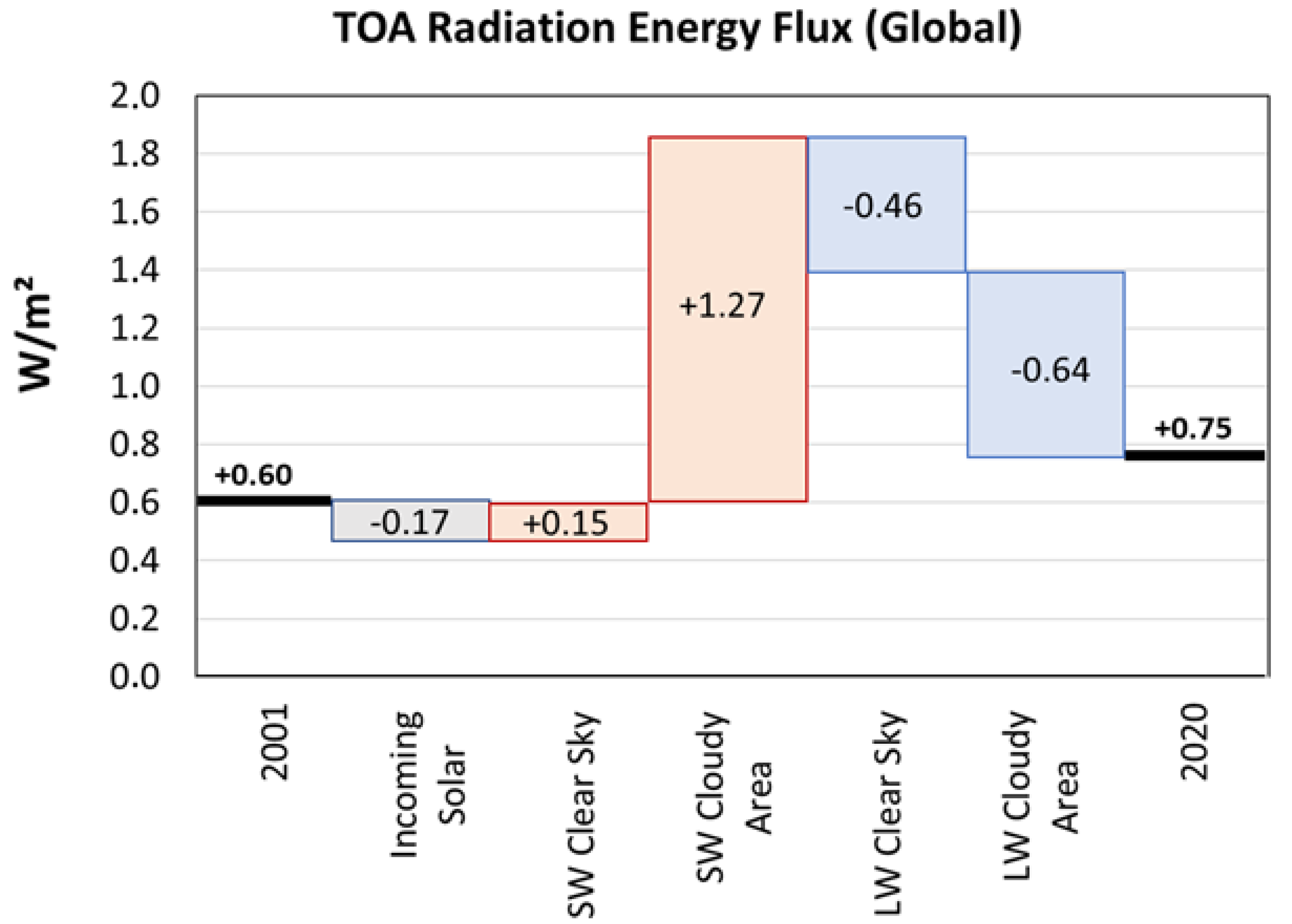
3. Results and Discussion: Top of Atmosphere (TOA) Radiative Balance
4. Results and Discussion: Surface Fluxes
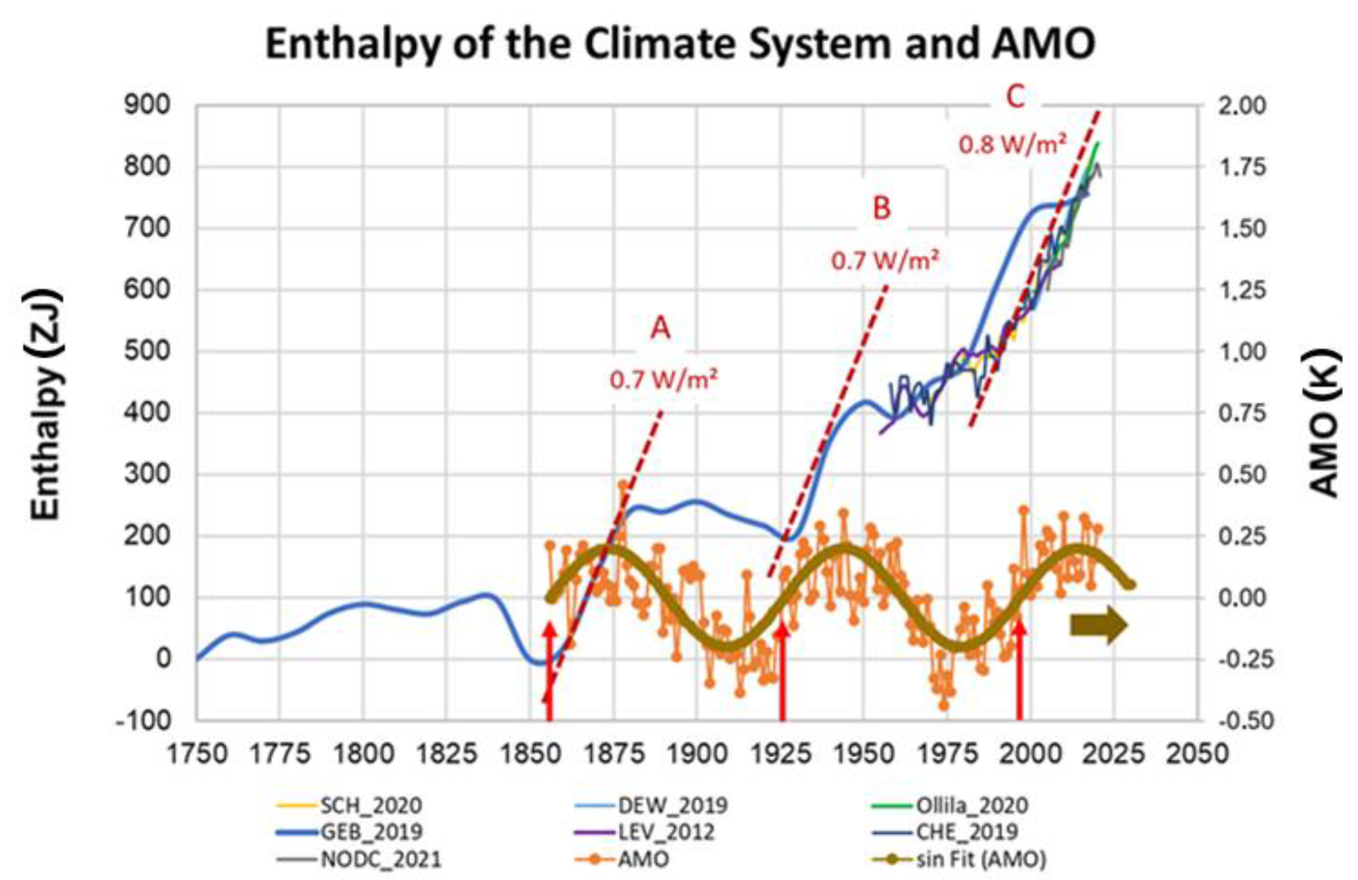
5. Effect on the Climate System’s Enthalpy
6. Conclusions
Author Contributions
Funding
Institutional Review Board Statement
Informed Consent Statement
Data Availability Statement
Acknowledgments
Conflicts of Interest
Appendix A
| Quantity | Intercept | Error of Intercept | Slope | Error of Slope | Trend | Rel. Error |
|---|---|---|---|---|---|---|
| Unit | W/m2 | W/m2 | W/m2 a | W/m2 a | W/m2 dec | % |
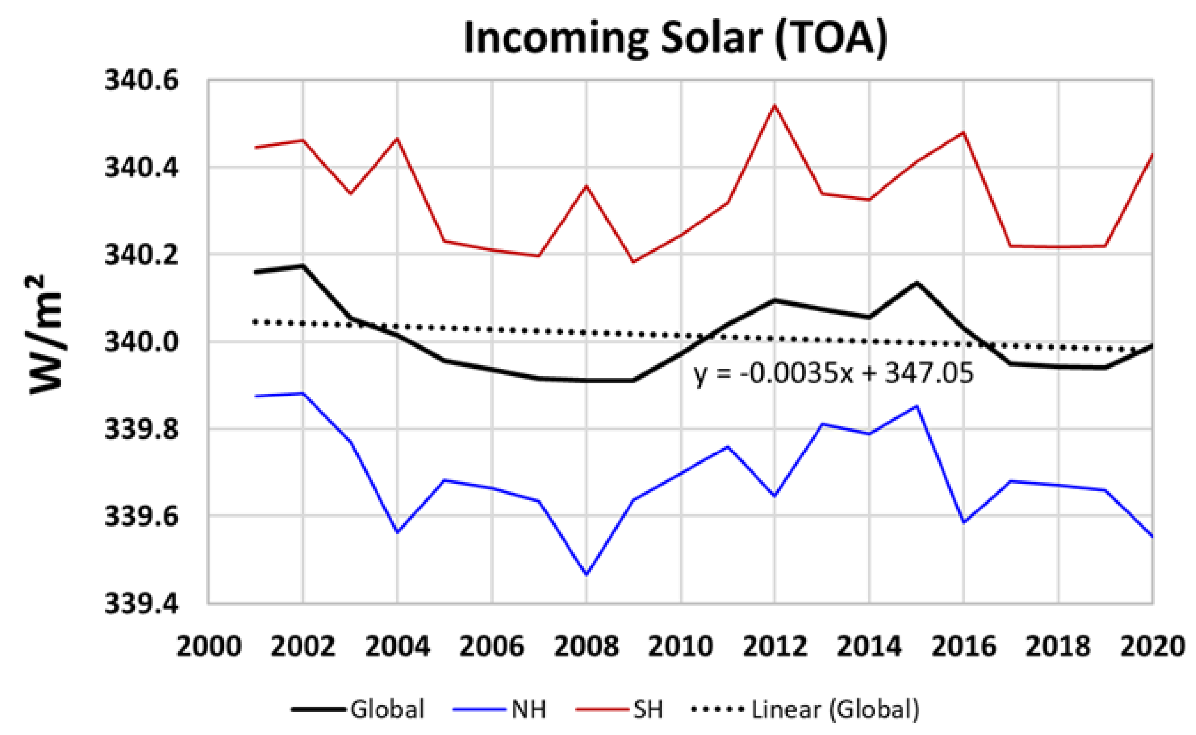
| Inc. Solar Flux in-TOA Global | 340.05 | 0.04 | −0.0035 | 0.0032 | −0.03 | 92 |
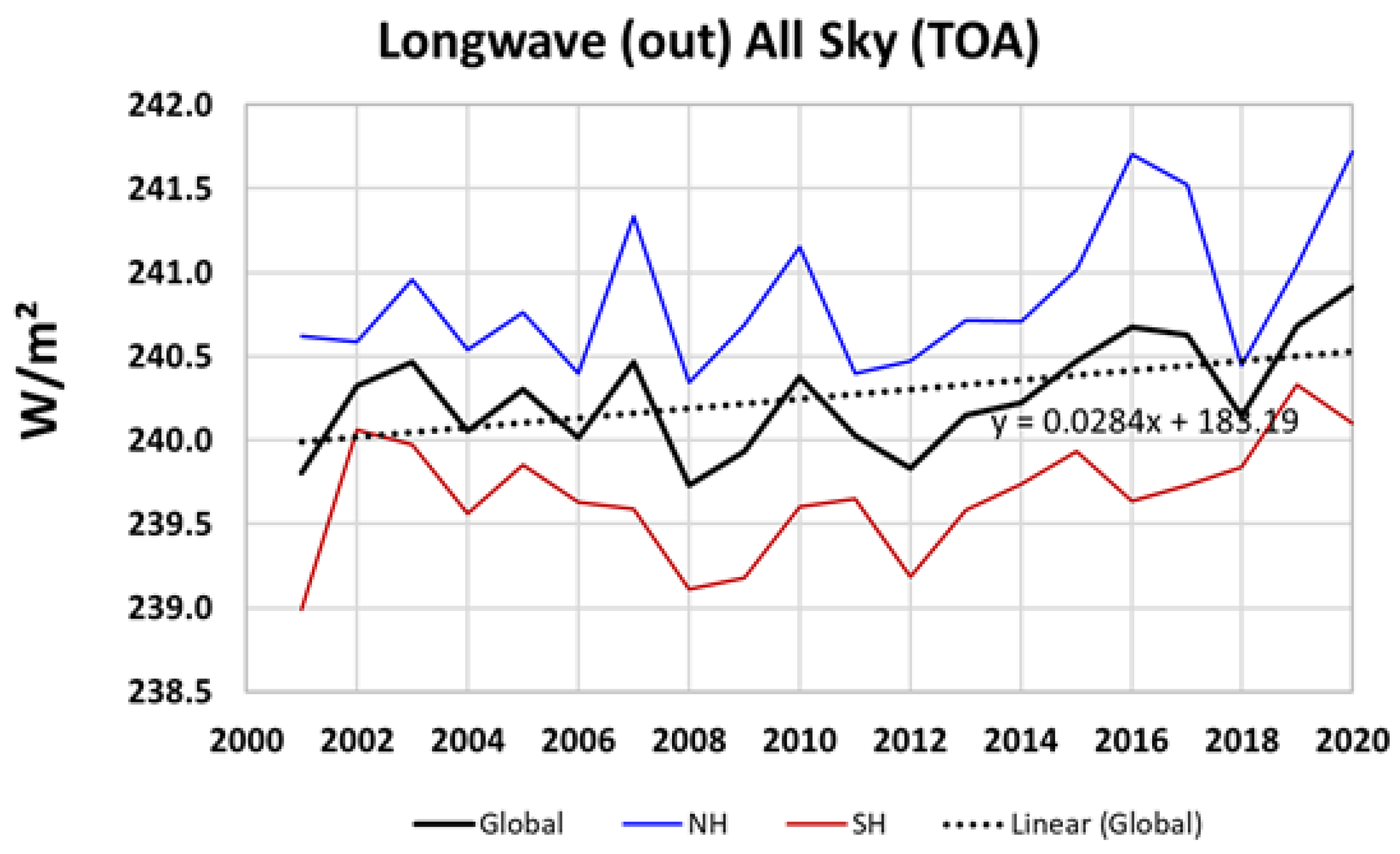
| LW Flux out-All Sky-TOA Global | 239.99 | 0.12 | 0.0284 | 0.0112 | 0.28 | 39 |
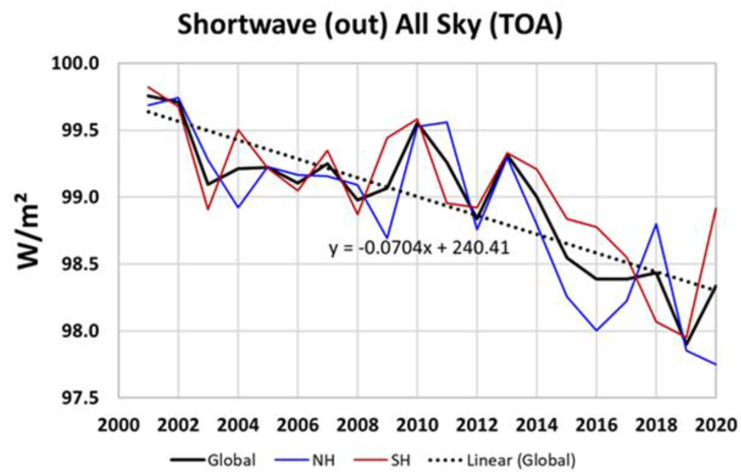
| SW Flux out-All Sky-TOA Global | 99.64 | 0.12 | −0.0704 | 0.0107 | −0.70 | 15 |
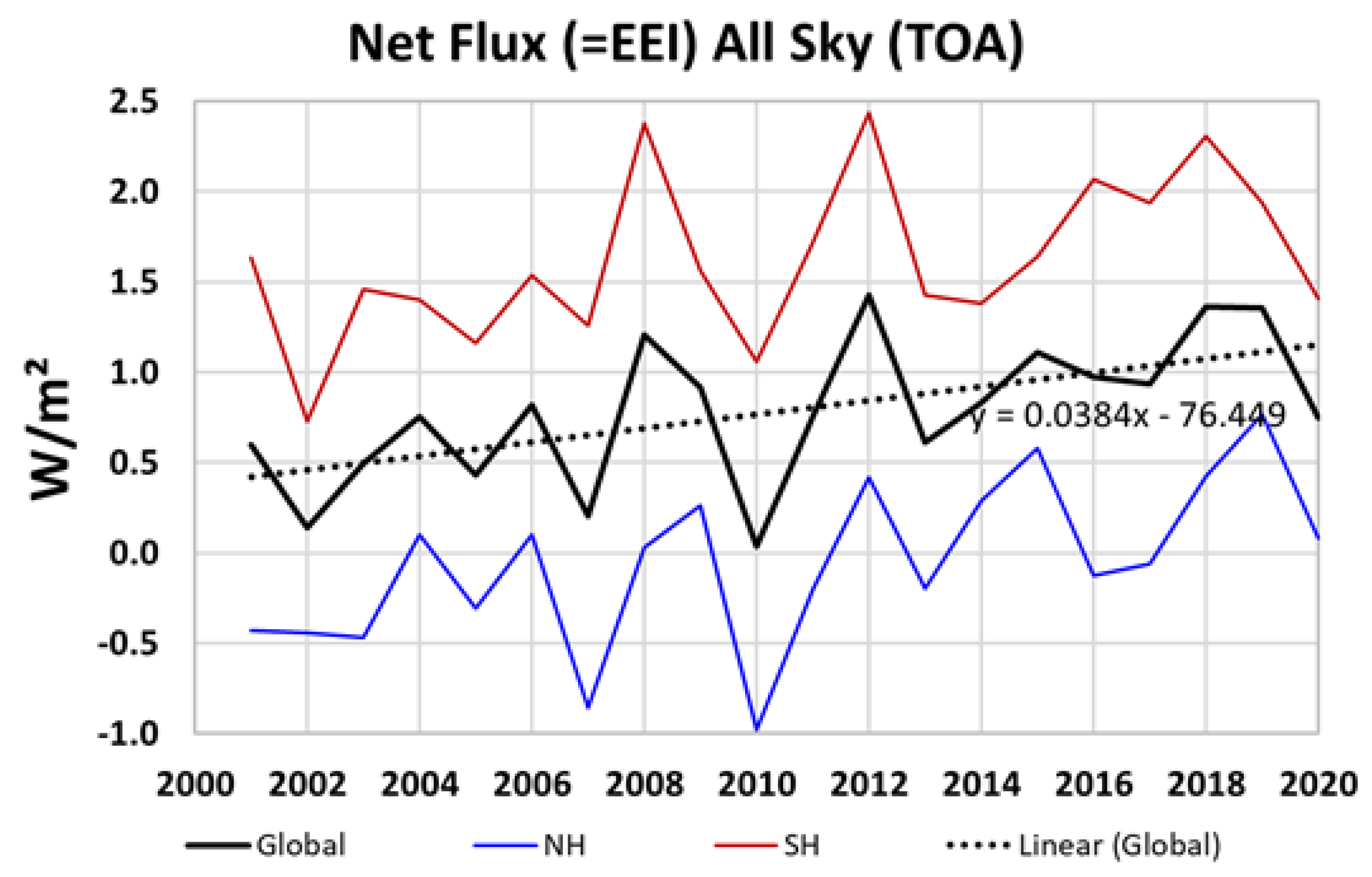
| Net Flux-All Sky-TOA Global | 0.42 | 0.14 | 0.0384 | 0.0130 | 0.38 | 34 |
| LW Flux out-Clear Sky-TOA Global | 268.14 | 0.11 | 0.0044 | 0.0102 | 0.04 | 229 |
| SW Flux out-Clear Sky-TOA Global | 53.61 | 0.07 | −0.0372 | 0.0066 | −0.37 | 18 |
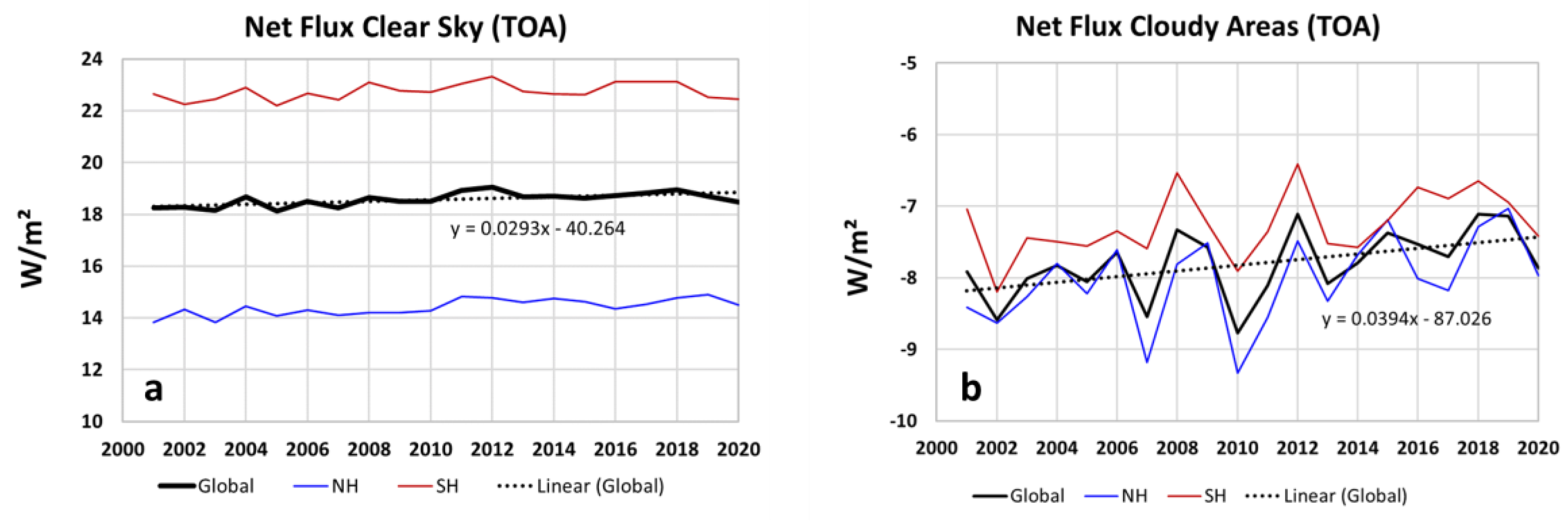
| Net Flux-Clear Sky-TOA Global | 18.30 | 0.09 | 0.0293 | 0.0080 | 0.29 | 27 |
| LW Flux out-Cloudy Areas-TOA Global | 226.45 | 0.15 | 0.0346 | 0.0134 | 0.35 | 39 |
| SW Flux out-Cloudy Areas-TOA Global | 121.77 | 0.16 | −0.0775 | 0.0142 | −0.78 | 18 |
| Net Flux-Cloudy Areas-TOA Global | −8.18 | 0.19 | 0.0394 | 0.0167 | 0.39 | 42 |
| Inc. Solar Flux in-TOA NH | 339.74 | 0.05 | −0.0048 | 0.0043 | −0.05 | 90 |
| LW Flux out-All Sky-TOA NH | 240.53 | 0.17 | 0.0344 | 0.0153 | 0.34 | 45 |
| SW Flux out-All Sky-TOA NH | 99.66 | 0.16 | −0.0813 | 0.0145 | −0.81 | 18 |
| Net Flux-All Sky-TOA NH | −0.45 | 0.17 | 0.0421 | 0.0151 | 0.42 | 36 |
| LW Flux out-Clear Sky-TOA NH | 268.87 | 0.14 | 0.0174 | 0.0129 | 0.17 | 74 |
| SW Flux out-Clear Sky-TOA NH | 56.83 | 0.10 | −0.0616 | 0.0086 | −0.62 | 14 |
| Net Flux-Clear Sky-TOA NH | 14.04 | 0.09 | 0.0393 | 0.0084 | 0.39 | 21 |
| LW Flux out-Cloudy Areas-TOA NH | 224.88 | 0.18 | 0.0469 | 0.0164 | 0.47 | 35 |
| SW Flux out-Cloudy Areas-TOA NH | 123.31 | 0.23 | −0.0969 | 0.0209 | −0.97 | 22 |
| Net Flux-Cloudy Areas-TOA NH | −8.45 | 0.25 | 0.0452 | 0.0221 | 0.45 | 49 |
| Inc. Solar Flux in-TOA SH | 340.35 | 0.05 | −0.0022 | 0.0045 | −0.02 | 203 |
| LW Flux out-All Sky-TOA SH | 239.45 | 0.14 | 0.0224 | 0.0128 | 0.22 | 57 |
| SW Flux out-All Sky-TOA SH | 99.61 | 0.15 | −0.0594 | 0.0134 | −0.59 | 22 |
| Net Flux-All Sky-TOA SH | 1.29 | 0.18 | 0.0348 | 0.0158 | 0.35 | 45 |
| LW Flux out-Clear Sky-TOA SH | 267.41 | 0.11 | −0.0085 | 0.0100 | −0.09 | 118 |
| SW Flux out-Clear Sky-TOA SH | 50.38 | 0.11 | −0.0129 | 0.0095 | −0.13 | 74 |
| Net Flux-Clear Sky-TOA SH | 22.56 | 0.13 | 0.0192 | 0.0118 | 0.19 | 61 |
| LW Flux out-Cloudy Areas-TOA SH | 227.82 | 0.17 | 0.0231 | 0.0154 | 0.23 | 67 |
| SW Flux out-Cloudy Areas-TOA SH | 120.09 | 0.12 | −0.0572 | 0.0111 | −0.57 | 19 |
| Net Flux-Cloudy Areas-TOA SH | −7.56 | 0.18 | 0.0319 | 0.0165 | 0.32 | 52 |
| Quantity | p-Value (Slope) | CI Low (Slope) | CI High (Slope) | ∆ CI (Slope) | R2 | Fig. |
|---|---|---|---|---|---|---|
| Unit | 1 | W/m2 a | W/m2 a | W/m2 a | 1 | - |
| Inc. Solar Flux in-TOA Global | 0.2937 | −0.010 | 0.003 | 0.014 | 0.06 | 1 |
| LW Flux out-All Sky-TOA Global | 0.0204 | 0.005 | 0.052 | 0.047 | 0.26 | 2 |
| SW Flux out-All Sky-TOA Global | 0.0000 | −0.093 | −0.048 | 0.045 | 0.71 | 3 |
| Net Flux-All Sky-TOA Global | 0.0086 | 0.011 | 0.066 | 0.055 | 0.33 | 4 |
| LW Flux out-Clear Sky-TOA Global | 0.6674 | −0.017 | 0.026 | 0.043 | 0.01 | 6 |
| SW Flux out-Clear Sky-TOA Global | 0.0000 | −0.051 | −0.023 | 0.028 | 0.64 | 5 |
| Net Flux-Clear Sky-TOA Global | 0.0019 | 0.012 | 0.046 | 0.034 | 0.42 | 8 |
| LW Flux out-Cloudy Areas-TOA Global | 0.0190 | 0.006 | 0.063 | 0.056 | 0.27 | 6 |
| SW Flux out-Cloudy Areas-TOA Global | 0.0000 | −0.107 | −0.048 | 0.059 | 0.62 | 5 |
| Net Flux-Cloudy Areas-TOA Global | 0.0299 | 0.004 | 0.075 | 0.070 | 0.24 | 8 |
| Inc. Solar Flux in-TOA NH | 0.2835 | −0.014 | 0.004 | 0.018 | 0.06 | 1 |
| LW Flux out-All Sky-TOA NH | 0.0378 | 0.002 | 0.067 | 0.064 | 0.22 | 2 |
| SW Flux out-All Sky-TOA NH | 0.0000 | −0.112 | −0.051 | 0.061 | 0.64 | 3 |
| Net Flux-All Sky-TOA NH | 0.0119 | 0.010 | 0.074 | 0.063 | 0.30 | 4 |
| LW Flux out-Clear Sky-TOA NH | 0.1943 | −0.010 | 0.045 | 0.054 | 0.09 | 6 |
| SW Flux out-Clear Sky-TOA NH | 0.0000 | −0.080 | −0.044 | 0.036 | 0.74 | 5 |
| Net Flux-Clear Sky-TOA NH | 0.0002 | 0.022 | 0.057 | 0.035 | 0.55 | 8 |
| LW Flux out-Cloudy Areas-TOA NH | 0.0104 | 0.012 | 0.081 | 0.069 | 0.31 | 6 |
| SW Flux out-Cloudy Areas-TOA NH | 0.0002 | −0.141 | −0.053 | 0.088 | 0.54 | 5 |
| Net Flux-Cloudy Areas-TOA NH | 0.0553 | −0.001 | 0.092 | 0.093 | 0.19 | 8 |
| Inc. Solar Flux in- -TOA SH | 0.6275 | −0.012 | 0.007 | 0.019 | 0.01 | 1 |
| LW Flux out-All Sky-TOA SH | 0.0962 | −0.004 | 0.049 | 0.054 | 0.15 | 2 |
| SW Flux out-All Sky-TOA SH | 0.0003 | −0.088 | −0.031 | 0.056 | 0.52 | 3 |
| Net Flux-All Sky-TOA SH | 0.0410 | 0.002 | 0.068 | 0.066 | 0.21 | 4 |
| LW Flux out-Clear Sky-TOA SH | 0.4062 | −0.030 | 0.013 | 0.042 | 0.04 | 6 |
| SW Flux out-Clear Sky-TOA SH | 0.1932 | −0.033 | 0.007 | 0.040 | 0.09 | 5 |
| Net Flux-Clear Sky-TOA SH | 0.1209 | −0.006 | 0.044 | 0.050 | 0.13 | 8 |
| LW Flux out-Cloudy Areas-TOA SH | 0.1521 | −0.009 | 0.055 | 0.065 | 0.11 | 6 |
| SW Flux out-Cloudy Areas-TOA SH | 0.0001 | −0.080 | −0.034 | 0.047 | 0.60 | 5 |
| Net Flux-Cloudy Areas-TOA SH | 0.0693 | −0.003 | 0.067 | 0.070 | 0.17 | 8 |
| Quantity | Intercept | Error of Intercept | Slope | Error Slope | Trend | Rel. Error |
|---|---|---|---|---|---|---|
| Unit | W/m2 | W/m2 | W/m2 a | W/m2 a | W/m2 dec | % |
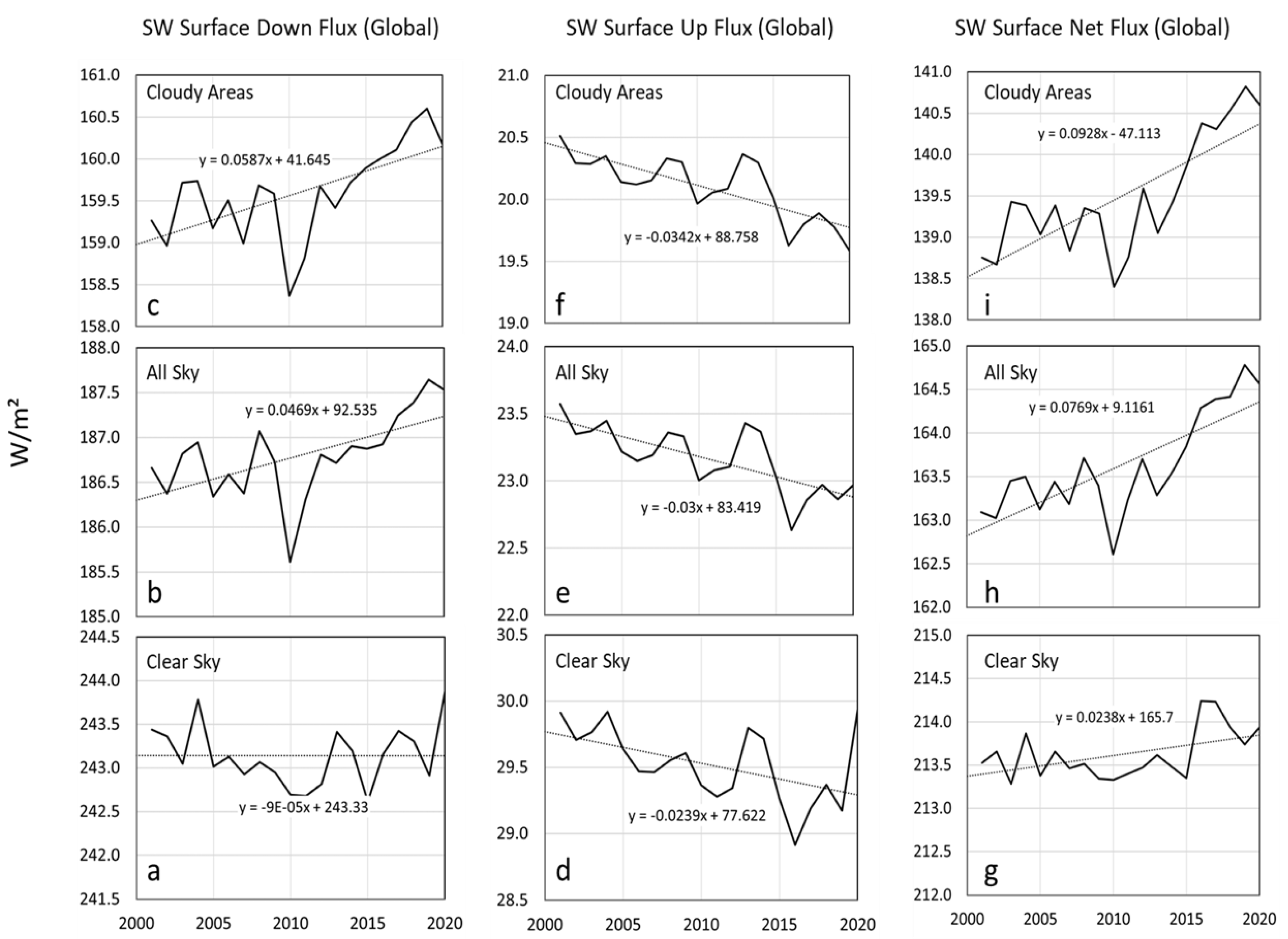
| SW Flux Down-All Sky-Surface Global | 186.35 | 0.17 | 0.047 | 0.015 | 0.47 | 32 |
| SW Flux Down-Clear Sky-Surface Global | 243.14 | 0.15 | 0.000 | 0.014 | 0.00 | 14723 |
| SW Flux Up-All Sky-Surface Global | 23.45 | 0.07 | −0.030 | 0.006 | −0.30 | 22 |
| SW Flux Up-Clear Sky-Surface Global | 29.75 | 0.11 | −0.024 | 0.010 | −0.24 | 41 |
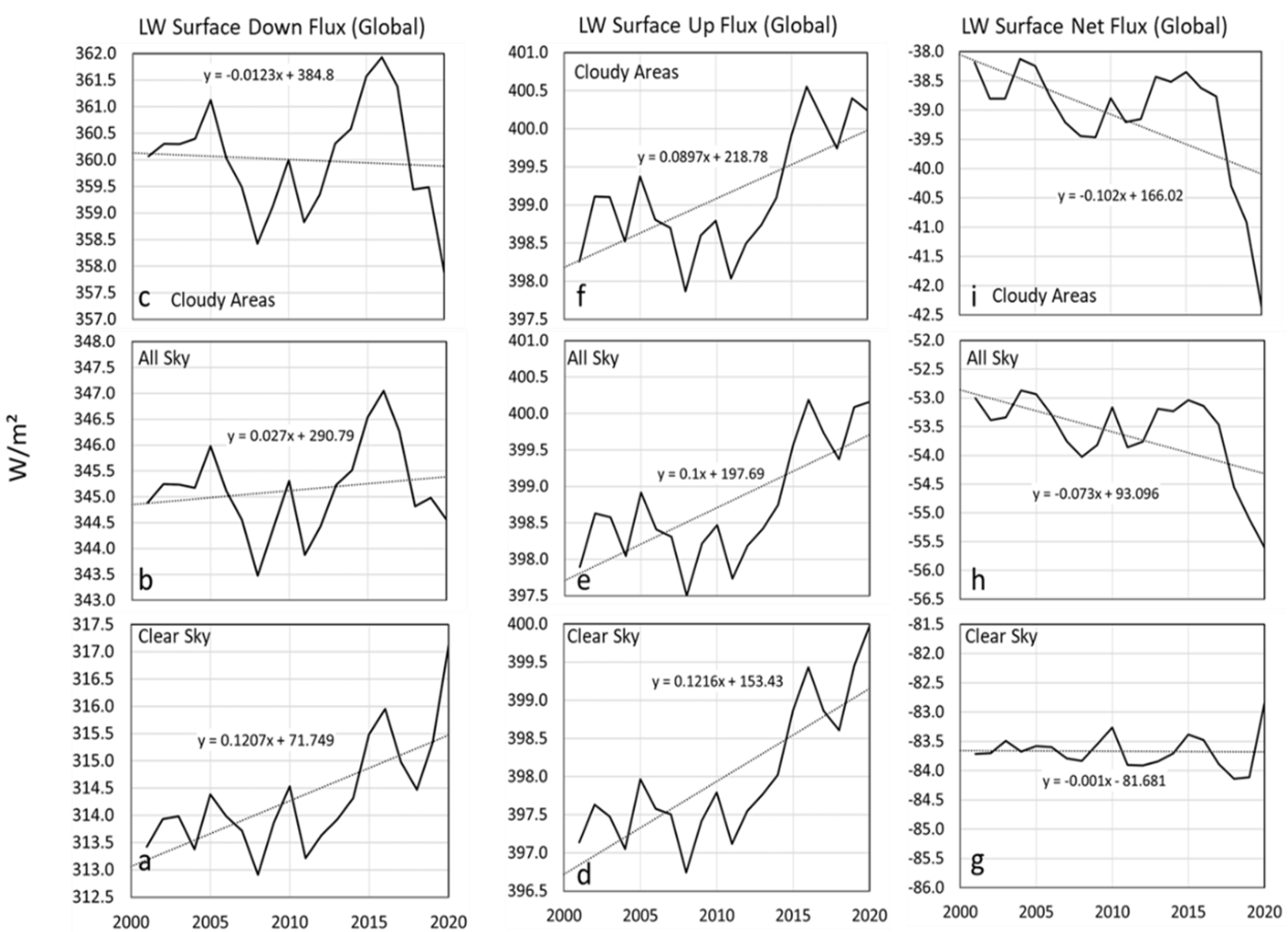
| LW Flux Down-All Sky-Surface Global | 344.88 | 0.37 | 0.027 | 0.034 | 0.27 | 125 |
| LW Flux Down-Clear Sky-Surface Global | 313.18 | 0.32 | 0.121 | 0.029 | 1.21 | 24 |
| LW Flux Up-All Sky-Surface Global | 397.81 | 0.25 | 0.100 | 0.023 | 1.00 | 23 |
| LW Flux Up-Clear Sky-Surface Global | 396.84 | 0.24 | 0.122 | 0.022 | 1.22 | 18 |
| SW Flux Down-Cloudy Areas-Surface Global | 159.04 | 0.19 | 0.059 | 0.017 | 0.59 | 29 |
| SW Flux Up-Cloudy Areas-Surface Global | 20.42 | 0.07 | −0.034 | 0.006 | −0.34 | 19 |
| LW Flux Down-Cloudy Areas-Surface Global | 360.12 | 0.46 | −0.012 | 0.041 | −0.12 | 335 |
| LW Flux Up-Cloudy Areas-Surface Global | 398.27 | 0.26 | 0.090 | 0.024 | 0.90 | 27 |
| SW Flux Net-All Sky-Surface Global | 162.90 | 0.16 | 0.077 | 0.015 | 0.77 | 19 |
| SW Flux Net-Clear Sky-Surface Global | 213.39 | 0.11 | 0.024 | 0.010 | 0.24 | 42 |
| SW Flux Net-Cloudy Areas-Surface Global | 138.61 | 0.20 | 0.093 | 0.018 | 0.93 | 19 |
| LW Flux Net-All Sky-Surface Global | −52.93 | 0.26 | −0.073 | 0.023 | −0.73 | 32 |
| LW Flux Net-Clear Sky-Surface Global | −83.66 | 0.13 | −0.001 | 0.012 | −0.01 | 1188 |
| LW Flux Net-Cloudy Areas-Surface Global | −38.15 | 0.37 | −0.102 | 0.033 | −1.02 | 33 |
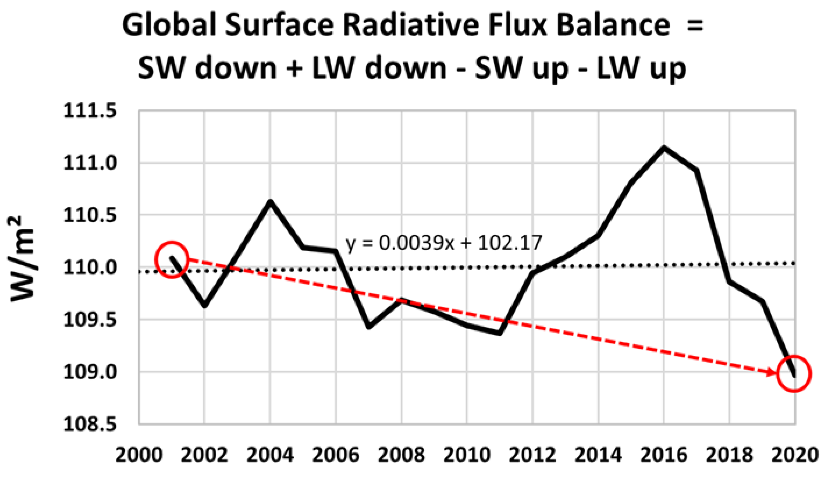
| LW + SW-All Sky-Surface Global | 109.96 | 0.25 | 0.004 | 0.022 | 0.04 | 579 |
| LW + SW-Clear Sky-Surface Global | 129.73 | 0.16 | 0.023 | 0.015 | 0.23 | 65 |
| LW + SW-Cloudy Areas-Surface Global | 100.46 | 0.37 | −0.009 | 0.034 | −0.09 | 364 |
| Quantity | p-Value (SLOPE) | CI Low (slope) | CI High (Slope) | ∆ CI (Slope) | R2 | Fig. |
|---|---|---|---|---|---|---|
| Unit | 1 | W/m2 a | W/m2 a | W/m2 a | 1 | - |
| SW Flux Down-All Sky-Surface Global | 0.0064 | 0.015 | 0.079 | 0.064 | 0.35 | 10 |
| SW Flux Down-Clear Sky-Surface Global | 0.9947 | −0.029 | 0.029 | 0.057 | 0.00 | 10 |
| SW Flux Up-All Sky-Surface Global | 0.0002 | −0.044 | −0.016 | 0.027 | 0.54 | 10 |
| SW Flux Up-Clear Sky-Surface Global | 0.0246 | −0.044 | −0.003 | 0.041 | 0.25 | 10 |
| LW Flux Down-All Sky-Surface Global | 0.4327 | −0.044 | 0.098 | 0.142 | 0.03 | 11 |
| LW Flux Down-Clear Sky-Surface Global | 0.0006 | 0.059 | 0.182 | 0.123 | 0.49 | 11 |
| LW Flux Up-All Sky-Surface Global | 0.0004 | 0.052 | 0.148 | 0.096 | 0.52 | 11 |
| LW Flux Up-Clear Sky-Surface Global | 0.0000 | 0.076 | 0.167 | 0.091 | 0.64 | 11 |
| SW Flux Down-Cloudy Areas-Surface Global | 0.0032 | 0.022 | 0.095 | 0.073 | 0.39 | 10 |
| SW Flux Up-Cloudy Areas-Surface Global | 0.0000 | −0.048 | −0.021 | 0.027 | 0.61 | 10 |
| LW Flux Down-Cloudy Areas-Surface Global | 0.7685 | −0.099 | 0.074 | 0.173 | 0.00 | 11 |
| LW Flux Up-Cloudy Areas-Surface Global | 0.0014 | 0.040 | 0.140 | 0.100 | 0.44 | 11 |
| SW Flux Net-All Sky-Surface Global | 0.0001 | 0.046 | 0.107 | 0.061 | 0.61 | 10 |
| SW Flux Net-Clear Sky-Surface Global | 0.0290 | 0.003 | 0.045 | 0.042 | 0.24 | 10 |
| SW Flux Net-Cloudy Areas-Surface Global | 0.0001 | 0.055 | 0.131 | 0.076 | 0.60 | 10 |
| LW Flux Net-All Sky-Surface Global | 0.0059 | −0.122 | −0.024 | 0.098 | 0.35 | 11 |
| LW Flux Net-Clear Sky-Surface Global | 0.9339 | −0.026 | 0.024 | 0.049 | 0.00 | 11 |
| LW Flux Net-Cloudy Areas-Surface Global | 0.0067 | −0.172 | −0.032 | 0.140 | 0.34 | 11 |
| LW + SW -All Sky-Surface Global | 0.8647 | −0.043 | 0.051 | 0.094 | 0.00 | 12 |
| LW + SW -Clear Sky-Surface Global | 0.1405 | −0.008 | 0.054 | 0.062 | 0.12 | - |
| LW + SW -Cloudy Areas-Surface Global | 0.7865 | −0.080 | 0.061 | 0.141 | 0.00 | - |
References
- Hansen, J.; Nazarenko, L.; Ruedy, R.; Sato, M.; Willis, J.; Del Genio, A.; Koch, D.; Lacis, A.; Lo, K.; Menon, S.; et al. Earth’s energy imbalance: Confirmation and implications. Science 2005, 308, 1431–1435. [Google Scholar] [CrossRef] [PubMed]
- Hansen, J.; Sato, M.; Kharecha, P.; von Schuckmann, K. Earth’s energy imbalance and implications. Atmos. Chem. Phys. 2011, 11, 13421–13449. [Google Scholar] [CrossRef]
- Trenberth, K.E.; Fasullo, J.T.; Balmaseda, M.A. Earth’s Energy Imbalance. J. Clim. 2014, 27, 3129–3144. [Google Scholar] [CrossRef]
- Dewitte, S.; Clerbaux, N. Measurement of the Earth Radiation Budget at the Top of the Atmosphere—A Review. Remote Sens. 2017, 9, 1143. [Google Scholar] [CrossRef]
- Kato, S.; Rose, F.G.; Rutan, D.A.; Thorsen, T.; Loeb, N.G.; Doelling, D.R.; Huang, X.; Smith, W.L.; Su, W.; Ham, S.-H. Surface Irradiances of Edition 4.0 Clouds and the Earth’s Radiant Energy System (CERES) Energy Balanced and Filled (EBAF) Data Product. J. Clim. 2018, 31, 4501–4527. [Google Scholar] [CrossRef]
- Loeb, N.G.; Doelling, D.R.; Wang, H.; Su, W.; Nguyen, C.; Corbett, J.G.; Liang, L.; Mitrescu, C.; Rose, F.G.; Kato, S. Clouds and the Earth’s Radiant Energy System (CERES) Energy Balanced and Filled (EBAF) Top-of-Atmosphere (TOA) Edition-4.0 Data Product. J. Clim. 2018, 31, 895–918. [Google Scholar] [CrossRef]
- Levitus, S.; Antonov, J.I.; Boyer, T.P.; Baranova, O.K.; Garcia, H.E.; Locarnini, R.A.; Mishonov, A.V.; Reagan, J.R.; Seidov, D.; Yarosh, E.S.; et al. World ocean heat content and thermosteric sea level change (0–2000 m), 1955–2010. Geophys. Res. Lett. 2012, 39. [Google Scholar] [CrossRef]
- Abraham, J.P.; Baringer, M.; Bindoff, N.; Boyer, T.; Cheng, L.; Church, J.A.; Conroy, J.L.; Domingues, C.M.; Fasullo, J.; Gilson, J.; et al. A review of global ocean temperature observations: Implications for ocean heat content estimates and climate change. Rev. Geophys. 2013, 51, 450–483. [Google Scholar] [CrossRef]
- Cheng, L.; Trenberth, K.E.; Fasullo, J.; Boyer, T.; Abraham, J.; Zhu, J. Improved estimates of ocean heat content from 1960 to 2015. Sci. Adv. 2017, 3, e1601545. [Google Scholar] [CrossRef]
- Cheng, L.; Zhu, J.; Abraham, J.; Trenberth, K.E.; Fasullo, J.T.; Zhang, B.; Yu, F.; Wan, L.; Chen, X.; Song, X. 2018 Continues Record Global Ocean Warming. Adv. Atmos. Sci. 2019, 36, 249–252. [Google Scholar] [CrossRef]
- Gebbie, G.; Huybers, P. The Little Ice Age and 20th-century deep Pacific cooling. Science 2019, 363, 70–74. [Google Scholar] [CrossRef]
- Meyssignac, B.; Boyer, T.; Zhao, Z.; Hakuba, M.Z.; Landerer, F.W.; Stammer, D.; Köhl, A.; Kato, S.; L’Ecuyer, T.; Ablain, M.; et al. Meas-uring Global Ocean Heat Content to Estimate the Earth Energy Imbalance. Front. Mar. Sci. 2019, 6, 432. [Google Scholar] [CrossRef]
- Von Schuckmann, K.; Cheng, L.; Palmer, M.D.; Hansen, J.; Tassone, C.; Aich, V.; Adusumilli, S.; Beltrami, H.; Boyer, T.; Cuesta-Valero, F.J.; et al. Heat stored in the Earth system: Where does the energy go? Earth Syst. Sci. Data 2020, 12, 2013–2041. [Google Scholar] [CrossRef]
- Loeb, N.G.; Johnson, G.C.; Thorsen, T.J.; Lyman, J.M.; Rose, F.G.; Kato, S. Satellite and Ocean Data Reveal Marked In-crease in Earth’s Heating Rate. Geophys. Res. Lett. 2021, 48, e2021GL093047. [Google Scholar] [CrossRef]
- Dewitte, S.; Clerbaux, N.; Cornelis, J. Decadal Changes of the Reflected Solar Radiation and the Earth Energy Imbalance. Remote Sens. 2019, 11, 663. [Google Scholar] [CrossRef]
- Loeb, N.; Thorsen, T.; Norris, J.; Wang, H.; Su, W. Changes in Earth’s Energy Budget during and after the “Pause” in Global Warming: An Observational Perspective. Climate 2018, 6, 62. [Google Scholar] [CrossRef]
- Wong, T.; Stackhouse Jr, P.W.; Kratz, D.P.; Sawaengphokhai, P.; Wilber, A.C.; Gupta, S.K.; Loeb, N.G. State of the Climate in 2019. Bull. Am. Meteorol. Soc. 2020, 101, S66–S69. [Google Scholar]
- Ollila, A. The Pause End and Major Temperature Impacts during Super El Niños are Due to Shortwave Radiation Anomalies. Phys. Sci. Int. J. 2020, 1–20. [Google Scholar] [CrossRef]
- Stephens, G.L. Cloud Feedbacks in the Climate System: A Critical Review. J. Clim. 2005, 18, 237–273. [Google Scholar] [CrossRef]
- Karlsson, K.-G.; Anttila, K.; Trentmann, J.; Stengel, M.; Solodovnik, I.; Meirink, J.F.; Devasthale, A.; Kothe, S.; Jääskeläinen, E.; Sedlar, J.; et al. CLARA-A2.1: CM SAF CLoud, Albedo and Surface RAdiation Dataset from AVHRR Data—Edition 2.1; EUMETSAT: Darmstadt, Germany, 2020. [Google Scholar] [CrossRef]
- Hartmann, D.L.; Ceppi, P. Trends in the CERES Dataset, 2000–2013: The Effects of Sea Ice and Jet Shifts and Comparison to Climate Models. J. Clim. 2014, 27, 2444–2456. [Google Scholar] [CrossRef]
- Svensmark, H. FORCEMAJEURE—The Sun’s Role in Climate Change; The Global Warming Policy Foundation: London, UK, 2019; ISBN 978-0-9931190-9-5. [Google Scholar]
- Shaviv, N.J. On climate response to changes in the cosmic ray flux and radiative budget. J. Geophys. Res. Space Phys. 2005, 110. [Google Scholar] [CrossRef]
- Roemmich, D.; A Church, J.; Gilson, J.; Monselesan, D.; Sutton, P.; Wijffels, S. Unabated planetary warming and its ocean structure since 2006. Nat. Clim. Chang. 2015, 5, 240–245. [Google Scholar] [CrossRef]
- Baggenstos, D.; Häberli, M.; Schmitt, J.; Shackleton, S.A.; Birner, B.; Severinghaus, J.P.; Kellerhals, T.; Fischer, H. Earth’s radiative imbalance from the Last Glacial Maximum to the present. Proc. Natl. Acad. Sci. USA 2019, 116, 14881–14886. [Google Scholar] [CrossRef] [PubMed]
- Allan, R.P.; Liu, C.; Loeb, N.G.; Palmer, M.D.; Roberts, M.; Smith, D.; Vidale, P.-L. Changes in global net radiative imbalance 1985–2012. Geophys. Res. Lett. 2014, 41, 5588–5597. [Google Scholar] [CrossRef]
- Wild, M. Global dimming and brightening: A review. J. Geophys. Res. Space Phys. 2009, 114, 114. [Google Scholar] [CrossRef]
- Liu, C.; Allan, R.P.; Mayer, M.; Hyder, P.; Loeb, N.G.; Roberts, C.; Valdivieso, M.; Edwards, J.M.; Vidale, P.-L. Evaluation of satellite and reanalysis-based global net surface energy flux and uncertainty estimates. J. Geophys. Res. Atmos. 2017, 122, 6250–6272. [Google Scholar] [CrossRef]
- Su, W.; Liang, L.; Wang, H.; Eitzen, Z.A. Uncertainties in CERES Top-of-Atmosphere Fluxes Caused by Chang-es in Accompanying Imager. Remote Sens. 2020, 12, 2040. [Google Scholar] [CrossRef]
- Johnson, G.C.; Lyman, J.M.; Loeb, N.G. Improving estimates of Earth’s energy imbalance. Nat. Clim. Chang. 2016, 6, 639–640. [Google Scholar] [CrossRef]
- Chylek, P.; Klett, J.D.; Lesins, G.; Dubey, M.K.; Hengartner, N. The Atlantic Multidecadal Oscillation as a dominant factor of oceanic influence on climate. Geophys. Res. Lett. 2014, 41, 1689–1697. [Google Scholar] [CrossRef]
- Kravtsov, S.; Grimm, C.; Gu, S. Global-scale multidecadal variability missing in state-of-the-art climate models. Npj Clim. Atmos. Sci. 2018, 1, 34. [Google Scholar] [CrossRef]
- Zhou, J.; Tung, K.-K. Deducing Multidecadal Anthropogenic Global Warming Trends Using Multiple Regression Analysis. J. Atmos. Sci. 2013, 70, 3–8. [Google Scholar] [CrossRef]
- Chen, J.; Carlson, B.E.; Del Genio, A.D. Evidence for Strengthening of the Tropical General Circulation in the 1990s. Science 2002, 295, 838–841. [Google Scholar] [CrossRef] [PubMed]
- Wielicki, B.A.; Wong, T.; Allan, R.P.; Slingo, A.; Kiehl, J.T.; Soden, B.J.; Gordon, C.T.; Miller, A.J.; Yang, S.-K.; Randall, D.A.; et al. Evidence for large decadal variability in the tropical mean radiative en-ergy budget. Science 2002, 295, 841–844. [Google Scholar] [CrossRef] [PubMed]
- Kubar, T.L.; Jiang, J.H. Net Cloud Thinning, Low-Level Cloud Diminishment, and Hadley Circulation Weak-ening of Precipitating Clouds with Tropical West Pacific SST Using MISR and Other Satellite and Reanalysis Data. Remote Sens. 2019, 11, 1250. [Google Scholar] [CrossRef]
- Del Genio, A.D.; Wolf, A.B. The Temperature Dependence of the Liquid Water Path of Low Clouds in the Southern Great Plains. J. Clim. 2000, 13, 3465–3486. [Google Scholar] [CrossRef]
- Gordon, N.D.; Klein, S.A. Low-cloud optical depth feedback in climate models. J. Geophys. Res. Atmos. 2014, 119, 6052–6065. [Google Scholar] [CrossRef]


Publisher’s Note: MDPI stays neutral with regard to jurisdictional claims in published maps and institutional affiliations. |
© 2021 by the authors. Licensee MDPI, Basel, Switzerland. This article is an open access article distributed under the terms and conditions of the Creative Commons Attribution (CC BY) license (https://creativecommons.org/licenses/by/4.0/).
Share and Cite
Dübal, H.-R.; Vahrenholt, F. Radiative Energy Flux Variation from 2001–2020. Atmosphere 2021, 12, 1297. https://doi.org/10.3390/atmos12101297
Dübal H-R, Vahrenholt F. Radiative Energy Flux Variation from 2001–2020. Atmosphere. 2021; 12(10):1297. https://doi.org/10.3390/atmos12101297
Chicago/Turabian StyleDübal, Hans-Rolf, and Fritz Vahrenholt. 2021. "Radiative Energy Flux Variation from 2001–2020" Atmosphere 12, no. 10: 1297. https://doi.org/10.3390/atmos12101297
APA StyleDübal, H.-R., & Vahrenholt, F. (2021). Radiative Energy Flux Variation from 2001–2020. Atmosphere, 12(10), 1297. https://doi.org/10.3390/atmos12101297