A Study on Synoptic Conditions Leading to the Extreme Rainfall in Taiwan during 10–12 June 2012

Abstract

During 10–12 June 2012, heavy rainfall occurred three days in a row in southern and central Taiwan, with daily rainfall maxima exceeding 500 mm on each day. In the Mei-yu season (May–June) during 1993–2000, only two other rainfall events had a comparable amount and duration, but this case was the only one that occurred well before the arrival of the Mei-yu front. The synoptic conditions and their evolution leading to this unique event are thus important and are the foci of this study. Our analysis indicates that the 10–12 June 2012 event in Taiwan was caused by the strong and persistent west-southwesterly low-level jet (LLJ) that transported warm, moist, and unstable air from upstream and then impinged on the island. The LLJ developed due to the enhanced horizontal pressure (or height) gradient when the pressure at low-levels fell significantly (by ~8 hPa) in South China (north of the jet) during 8–10 June, but the subtropical high to the southeast maintained its strength. Further, through a diagnosis using the pressure tendency equation, it is found that both warm air advection and the dynamic effects (column divergence and transport of mass by vertical motion) contributed to the pressure fall in South China. The warm air advection occurred in the southern part of a large-scale confluent pattern in China, and the persistent west-southwesterly flow through deep layer (mainly above 800 hPa) in South China transported warmer and less dense air into the region from lower latitudes. On the other hand, South China was also located under the diffluent zone in the northeastern quadrant of the South Asian upper-level anticyclone, which strengthened during 5–10 June and provided divergence aloft, which exceeded the low-level convergence and upward transport of mass (at a fixed height) into the column by vertical motion on 9 June. As a result, the dynamic effects also contributed to the pressure fall, although secondary to the warm air advection. The destabilization process in South China during 8–10 June was also helpful to increase convective activity and upper-level divergence.

1. Introduction

In early summer, during the seasonal transition from the cold dry northeasterly winter monsoon to the warm moist southwesterly summer monsoon, slow-moving fronts often form between the weakening continental Siberia high pressure system and the subtropical high over the western Pacific in many parts of East Asia [1]. These fronts bring a rainy season called the Mei-yu season around May–June in Taiwan and South China [2,3,4,5], and later in the season in Central China, Japan, and Korea [1,3,4] (cf. Figure 1). During this season in Taiwan, heavy rainfall often occur [5,6]. Typically, the Mei-yu front appear as a long belt of stratiform clouds extending thousands of kilometer on satellite imageries, with severe organized convection embedded inside, e.g., [7,8]. Chen and Chi [9] studied the relationship between Mei-yu fronts and rainfall in Taiwan and concluded that the rainfall in northern Taiwan can occur anywhere from 400 km south (ahead) of the front to 300 km north (behind it), and that in southern Taiwan can take place from 500 km south to 200 km north of the front. Thus, when a Mei-yu front approaches, nowhere in Taiwan is without the potential of heavy rainfall [9].

Many previous case studies have shown that heavy rainfall during the Mei-yu season in Taiwan are caused by organized mesoscale convective systems (MCSs), which form in favorable environments associated with the front and under sufficient mesoscale forcing [10,11,12,13,14]. One such feature commonly seen is the low-level jet (LLJ), which transports moisture toward the frontal zone [2,5,9] and may result from an enhanced horizontal pressure gradient across a front that exhibits appreciable baroclinicity through geostrophic adjustment process [5,15]. In other cases, the front near Taiwan may have a quasi-equivalent barotropic structure and be initially weak and shallow (e.g., [16]). As found by Chen et al. [17,18,19], the deep convection along and near the front can lead to cross-frontal convergence, and thus frontogenesis, at low levels through a mechanism similar to the Conditional Instability of the Second Kind (also [20]). In these cases, LLJs can also form south of the front in the lower branch of the cross-frontal transverse circulation through Coriolis torque, and in turn help to supply moisture and support the MCSs. Regardless the mechanism of LLJ development, once formed upstream from Taiwan, these MCSs can move over land with the environmental flow and subsequently produce heavy rainfall.

Chien and Hung [21] examined the climatological relationship between southwesterly flow and the rainfall in Taiwan. They found that when the low-level southwesterly flow is persistent, there often exists an anomalous low pressure system in South China, and this low contributes to a stronger wind speed and helps the convection to move into Taiwan from upstream areas (cf. Figure 1). When the LLJ has its source from the Bay of Bangle, its abundant moisture often also promote heavy rainfall in Taiwan (e.g., [22]). Many of the above studies show that heavy rainfall can occur in Taiwan when the Mei-yu front moves close, and the development and maintenance of the MCSs that lead to heavy rainfall are often closely linked to the southwesterly flow, the LLJs, and their moisture supply.

During 10–15 June 2012, widespread heavy rainfall occurred in Taiwan under the influence of an approaching Mei-yu front. The mountain interior, northern, and western Taiwan were among the regions mostly affected, as flooding and landslides took place in many areas. This was also the first time in the Mei-yu season in Taiwan that the Central Emergency Operation Center (EMOC) was established during the event to mitigate its weather hazards. In total, the event caused losses up to NTD 550 million in agriculture (~USD 20 million), 136 landslides and floods at 181 locations (source: National Center for Disaster Reduction, Global Disaster Event Book; https://den.ncdr.nat.gov.tw/1132/1188/1204/2339/2366, accessed on 24 June 2021). An early survey by the authors (

Table 1. Mei-yu heavy rainfall events (in May–June) that reached a peak daily rainfall amount of ≥350 mm for at least three days in a row during 1993–2020.

Year and Month	Date	No. of Gauges ≥350 mm	Time of Front to Reach Northern Taiwan
2005, June	12	10	0600 UTC 12 June 2005
	13	4
	14	8
	15	2
2006, June	8	1	1200 UTC 8 June 2006
	9	35
	10	7
2012, June	10	13	0600 UTC 12 June 2012
	11	15
	12	14

) shows that only three Mei-yu events (in May–June) reached a peak rainfall amount of ≥350 mm three days in a row during 1993–2020: 12–15 June 2005, 8–10 June 2006, and 10–12 June 2012. The last event is the present case. It was unique in that the Mei-yu front was still quite far from Taiwan in 10 and much of 11 June, whereas heavy rainfall took place when the front had already approached Taiwan in the first two events. Such interesting aspects will be shown shortly.

For the present event, Wang et al. [23] investigated the extreme rainfall over the Taipei Metropolitan Area in northern Taiwan (510 mm in 12 h) from late 11 to early 12 June 2012 using a cloud-resolving model. In their simulation, even with high resolution, the model could not reproduce the pre-frontal squall line that caused the first several hours of rainfall (due to high nonlinearity of the system). However, the same simulation successfully captured the rainband across northern Taiwan that was responsible for rainfall during the subsequent hours (peaking at 311 mm). Moreover, pre-frontal (except near the end), this second rainband formed along a low-level convergence zone arising due to the blocking effect of Taiwan’s topography on southwesterly flow. Inside the rainband, back-building behavior was observed, and both dynamic and thermodynamic effects associated with the developing cells to promote such a behavior, which were examined and discussed in [23]. Nevertheless, the synoptic pattern and the mechanisms and factors involved to lead to this unique event in Taiwan, with heavy rainfall over three consecutive days, are barely studied in the literature (e.g., [24]). To fill this gap in our knowledge, the goal of the present study therefore is to answer the question why heavy rainfall occurred in southern Taiwan well before the arrival of the surface Mei-yu front? To achieve this goal, the data used and our methodology are described in Section 2, and synoptic conditions are analyzed in Section 3. In Section 4, the pressure tendency equation is employed to further shed light on the important mechanisms involved. Section 5 provides our discussion on the findings, and finally the conclusion is given in Section 6.

2. Data and Methodology

2.1. Data

The data utilized in this study include the following: (1) Surface weather charts every 6 h (at 0000, 0600, 1200, and 1800 UTC) in May–June of 2005, 2006, and 2012 from the Japan Meteorological Agency (JMA), (2) European Center for Medium-range Weather Forecasts (ECMWF) global reanalysis (ERA-Interim) at 6-h intervals [25], on a 1° × 1° latitude/longitude grid at 36 pressure (p) levels, (3) the gridded Tropical Rainfall Measuring Mission (TRMM) data from National Aeronautics and Space Administration (NASA), USA (0.25° × 0.25° and every 3 h; [26]), and (4) rain-gauge data during Mei-yu season of 1993–2020 from a dense network operated and maintained by the Central Weather Bureau (CWB) in Taiwan [27]. The JMA weather charts and ERA-Interim are for synoptic analysis and diagnosis, while the latter dataset include all basic variables such as geopotential height, temperature, horizontal wind components, humidity, vertical motion, relative vorticity, horizontal divergence, and surface pressure, etc. The CWB gauge data are for the analysis of local rainfall in Taiwan [27]. From 1993 to 2000, the total number of gauges gradually increased. To avoid potential bias toward later events due to unequal sites, only those with records ≥80% of the total period were used (235 sites), and the results are already shown in Table 1. For rainfall over upstream and larger areas, TRMM data are used.

2.2. Methodology and the Pressure Tendency Equation

As will be shown later in Section 3, during the present case, the horizontal pressure gradient at low-levels strengthened to the south of the Mei-yu front, causing the LLJ to intensify, largely in response to considerable pressure fall over South China. Thus, the pressure tendency equation is employed to diagnose this pressure fall in Section 4. This equation is derived by integrating the hydrostatic equation dp = −ρ g dz, where ρ is air density, g is gravitational acceleration, and z is height, respectively, from a fixed height h to the top of the atmosphere, then take the partial derivative with respective to time (t) and use the continuity equation to get:

$$\frac{\partial p\left(h\right)}{\partial t}=-g{\int }_h^{\infty }\rho \left(\nabla ·\stackrel{\rightharpoonup }{V}\right)dz-g{\int }_h^{\infty }\left(\stackrel{\rightharpoonup }{V}·\nabla \rho \right)dz+g{\left(\rho w\right)}_h$$

(1)

where ∇ = (∂/∂x) i + (∂/∂y) j is the horizontal gradient operator, while i and j are the unit vectors in x and y direction, respectively, $\stackrel{\rightharpoonup }{V}$ = u i + v j is the horizontal wind vector, and w = dz/dt is the vertical velocity. From Equation (1), one sees that the pressure tendency at any given height h on the left hand side is contributed by three terms on the right hand side: total column-integrated net convergence (at and above h), total column-integrated net density advection, and upward transport of air mass at h from below. From the ideal gas law, it is clear that the positive density advection corresponds to cold air advection, so the three terms on the right hand side will simply be referred to as the convergence/divergence effect, temperature advection effect, and vertical motion effect (or term), respectively. While it might not be apparent, any warming/cooling effect other than the advection would be implicitly included in the convergence/divergence term, since temperature changes affect thickness and pressure through hydrostatic response. For example, persistent latent heating would lead to pressure rise and divergence aloft, and subsequently pressure drop at low levels. The ERA-Interim dataset is used for this calculation, for the domain shown in Figure 1 (red box). The height of h is chosen to be that at 950 hPa to avoid the influence of the hilly topography in South China (cf. Figure 1), while the top level is set at 150 hPa near the tropopause [28,29]. This level also showed limited variation in height, much smaller than those at low levels, during our case period. In practice, the convergence/divergence term is one order of magnitude larger than the tendency and advection terms, and cannot be computed with enough accuracy. Therefore, it is estimated as the residual of the three other terms, and as a result it is always nearly cancelled (balanced) by the vertical motion effect, as required to yield the correct pressure tendency values. For the same reason, no attempt is made to further partition the convergence/divergence effect into those from different sources, e.g., adiabatic and diabatic effects.

It is well-known that the semi-diurnal pressure tide is quite pronounced in subtropical regions such as South China, so its effects need to be removed from the terms in Equation (1) in order to reveal the signals at longer time scales. For this purpose, ERA-Interim data over a longer period from 0000 UTC 5 to 1800 UTC 16 June 2012 (12 days) are averaged to obtain the mean and averaged departures from this mean at each time of 0000, 0600, 1200, and 1800 UTC, respectively. Then, these departure values are subtracted from the original time series data based on the local time to remove the semi-diurnal tide. In cases where diurnal variations, instead of semi-diurnal ones, need to be removed (not limited to p), the same procedure is used.

3. Analysis on Synoptic Evolution

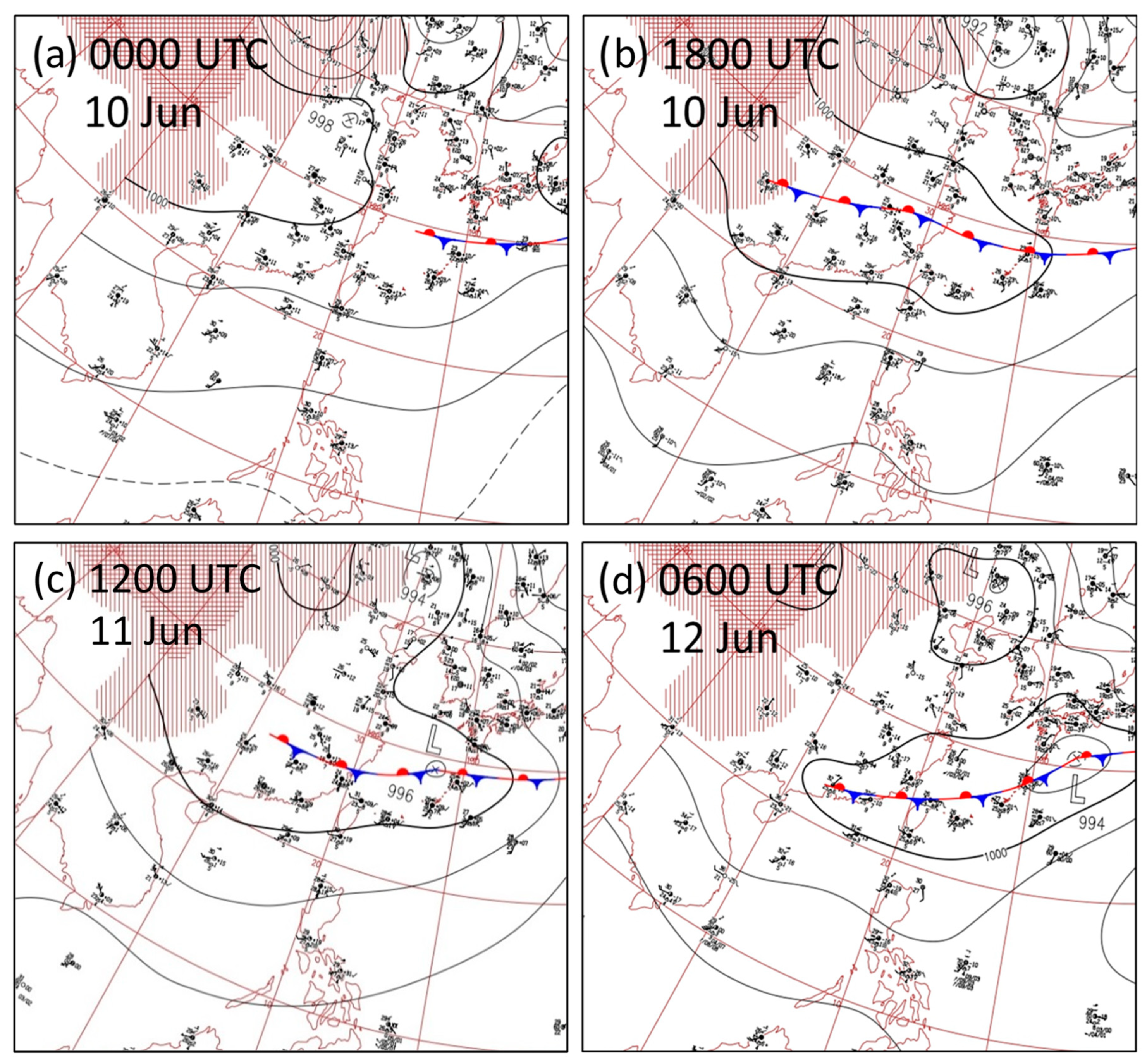
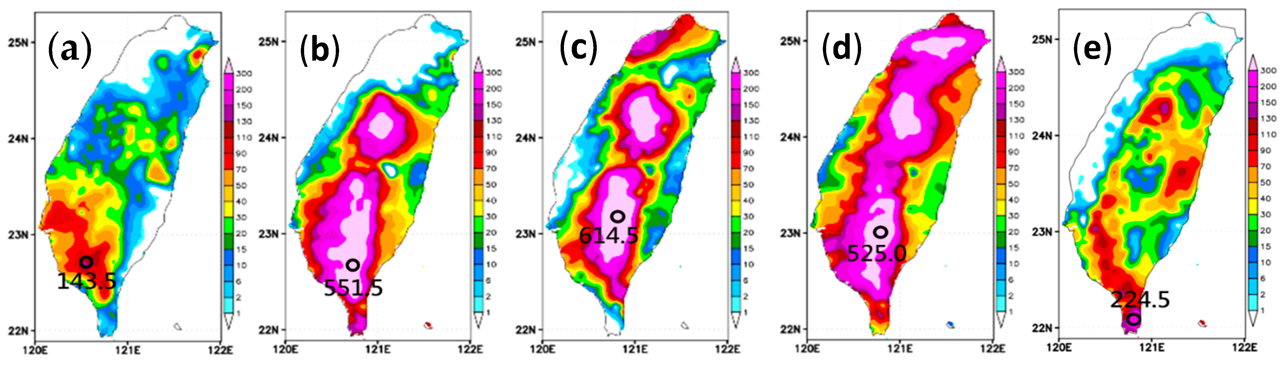
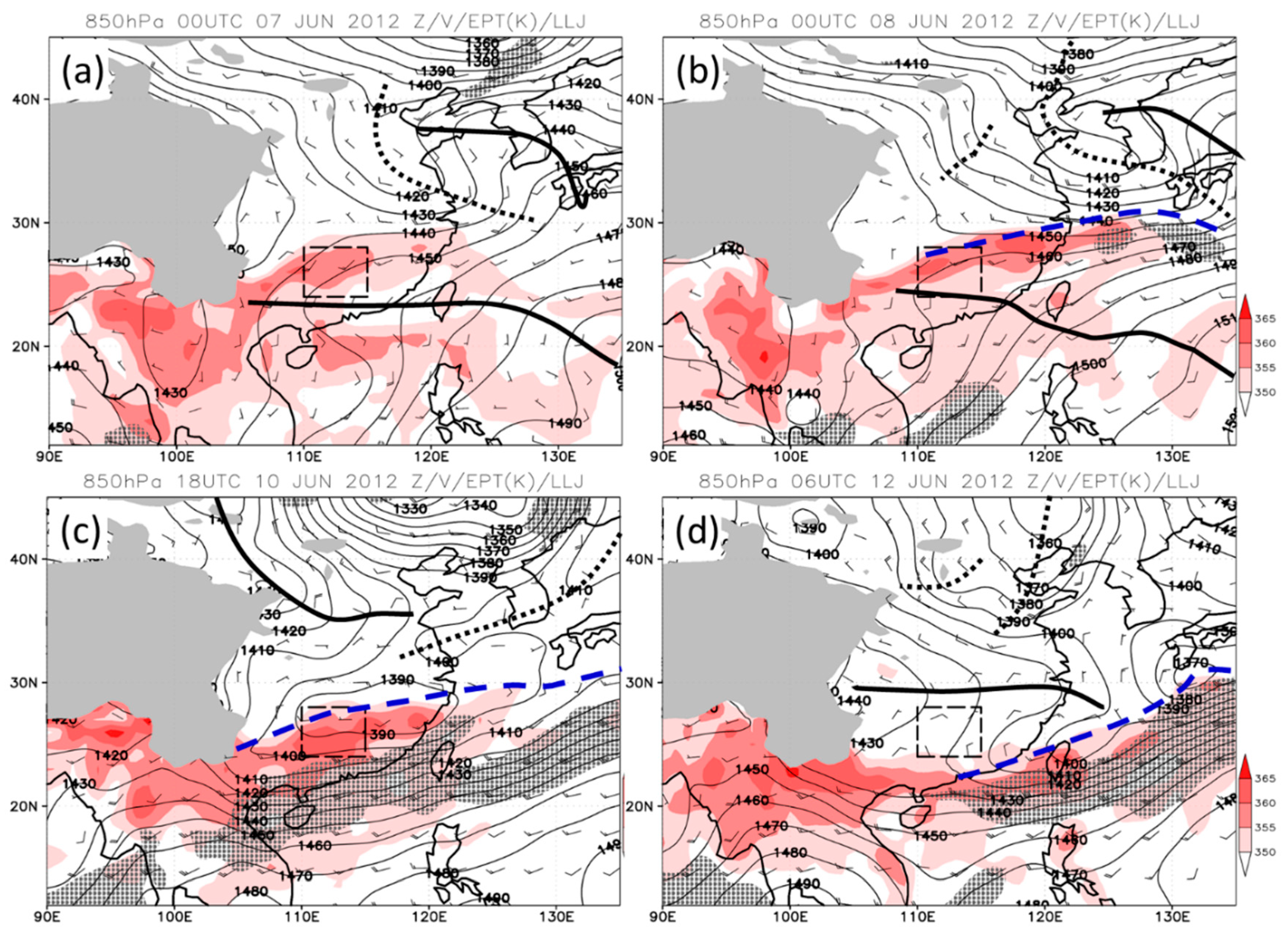
3.1. Position of Mei-yu Front during Heavy Rainfall

The JMA surface weather maps at selected times during the event are presented in Figure 2. At 0000 UTC 10 June (Figure 2a), an east-west oriented front was located over the East China Sea and south of Japan and moving eastward. With generally lower pressure over China and higher pressure toward the south and southeast, southwesterly flow prevailed near Taiwan. A second front appeared near 28°–29° N at 1800 UTC 10 June and extended all the way from southwestern China to the western North Pacific (Figure 2b), and remained quite far (>300 km) from Taiwan until 1200 UTC 11 June (Figure 2c), when it started to move southward. It reached northern Taiwan at 0600 UTC 12 June (Figure 2d), as mentioned (cf. Table 1), and quickly swept through much of the island on the same day (through 0000 UTC 13 June, not shown).

Figure 3 presents the spatial distribution of daily rainfall in Taiwan from 9 to 13 June 2012. On 9 June, considerable amounts of rainfall (peaking at 143.5 mm) was already received in southwestern Taiwan (Figure 3a). However, the rainfall increased dramatically during the three following days on 10–12 June, not only in southwestern plains but mainly in island interiors and reaching a maximum of 551.5, 614.5, and 525 mm, respectively (Figure 3b–d). While the extreme rainfall in northern Taiwan over 11–12 June was mainly from two pre-frontal rainbands as reviewed earlier [23] and obviously occurred closer to the front, those rainfall regions in central and southern Taiwan took place far south of the front, especially near the rainfall centers (all in southern Taiwan) during 10–11 June. Thus, compared to the other two events given in Table 1, the present case is unique in its own right that such extreme rainfall occurred over a lengthy period well to the south of the front and is worthy of detailed examination. After the surface front had moved south, the rainfall reduced on 13 June, but a peak amount of 224.5 mm still occurred at the southernmost part of Taiwan (Figure 3e).

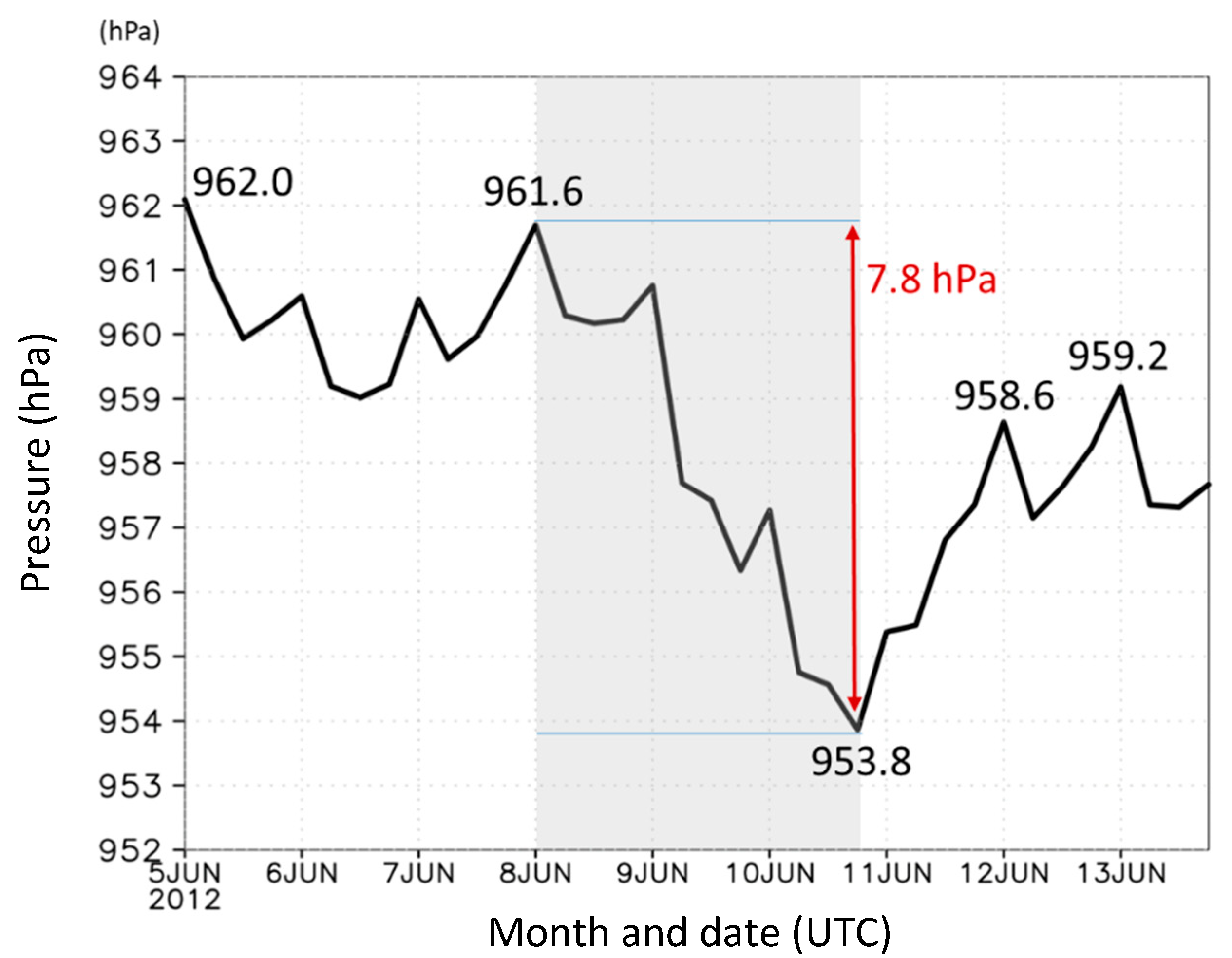
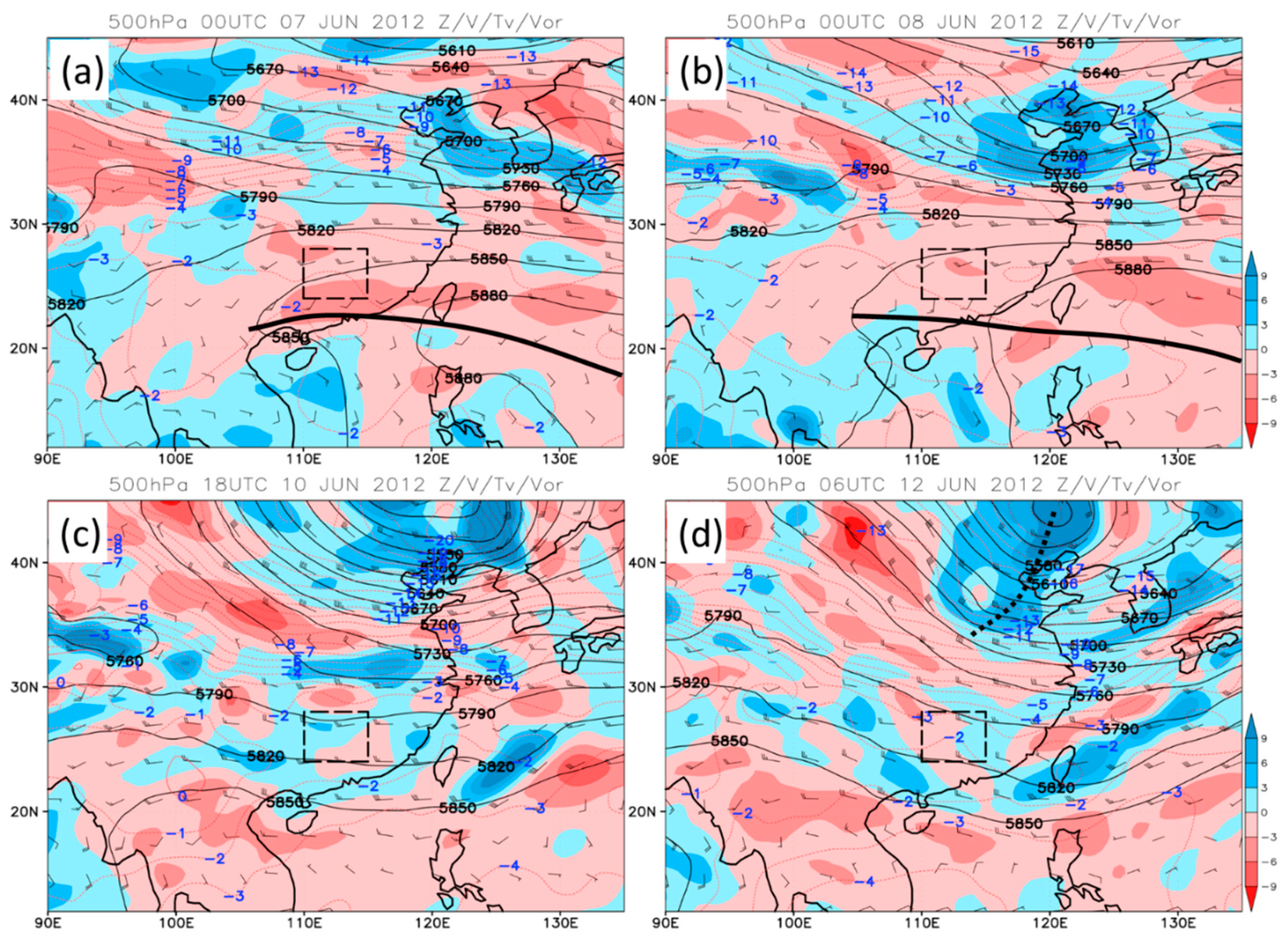
3.2. Pressure Fall in South China and Synoptic Evolution

Concurrent with the development of the Mei-yu front depicted in Figure 2, large areas in South China experienced considerable pressure fall at low levels. The time series of surface pressure (Figure 4) averaged over the rectangular area of 24°–28° N, 110°–115° E (red box in Figure 1) shows some decrease in value and recovery during 5–7 June, then significant drop from 961.6 to 953.8 hPa from 0000 UTC 8 to 1800 UTC 10 June (by 7.8 hPa). Afterwards, the areal-mean surface pressure in South China rose again to 959.2 hPa at 0000 UTC 13 June 2012 (Figure 4). Based on Figure 4, the period from 0000 UTC 8 to 1800 UTC 10 June is defined as the period of pressure fall, and its cause will be diagnosed using the pressure tendency equation later in Section 4.

The low-level synoptic weather conditions at 850 hPa at selected times from before to after the pressure fall (in South China) are shown in Figure 5. Before the event at 0000 UTC 7 June (Figure 5a), the ridge of the subtropical high (STH) extended from the southeast into Taiwan, then westward farther into China roughly along 23° N. North of this ridge, southwesterly flow prevailed over much of South China with relatively high values of equivalent potential temperature (θ_e; over 350 K). North of the Yangtze River Valley (YRV, along about 30 °N), northwesterly flow existed over much of Central China, thus forming a region of confluence roughly near and along the YRV (Figure 5a). This basic confluent pattern remained at 0000 UTC 8 June when a surface front (blue dashed line) moved through South China and the East China Sea (Figure 5b). At an elongated zone immediately south of the front, higher θ_e values also existed at 850 hPa. While the ridge position of the STH changed little, the horizontal gradients of geopotential height near Taiwan had started to strengthen with increased wind speed. By 1800 UTC 10 June when a second front developed in South China (Figure 5c), a corresponding low with a closed geopotential height contour also appeared and the contours continued to tighten along a zone roughly 500–1000 km south of the front. In agreement with this, a LLJ had formed at this time, with strong west-southwesterly winds ≥12.5 m s⁻¹ (stippled) extending from northern Vietnam to Taiwan and areas farther east. North of the Mei-yu front in Central China, a ridge had developed near 35° N and the winds turned into northeasterly at 850 hPa (Figure 5c). From Figure 5b to Figure 5c, the mean geopotential height in South China (dashed box) fell from about 1460 to 1390 gpm, but only about half the amount at the periphery of the STH, thus the height contours became tighter at low levels during the pressure fall period (in South China) of almost 3 days.

Later around 1200 UTC 11 June, the front started to move south more rapidly as discussed. At 0600 UTC 12 June, the surface front reached northern Taiwan and the area to its south continued to possess higher θ_e values, likely reflecting more abundant moisture. In Figure 5d, the ridge behind the front also moved south into the YRV (Figure 5d), leading to a pressure rise in South China by about 5 hPa (cf. Figure 4). The LLJ also moved south and east, but the winds speed was still strong near southern Taiwan and regions farther east (Figure 5d). Clearly, the strong west-southwesterly LLJ with high θ_e values was impinging on Taiwan and its steep topography during 10–12 June to cause the heavy rainfall. Based on several previous studies, the synoptic environment and abundant moisture near and ahead of the front were both favorable for heavy rainfall in Taiwan [11,30,31].

At 500 hPa in the middle-upper troposphere, a similar confluent flow pattern existed in Central and South China during 7–8 June 2012 (Figure 6a,b), with the STH in the WNP and a deepening trough around 120° E from part of Central to North China. The ridge line from STH still extended to regions just south of Taiwan, and west-southwesterly flow prevailing in much of South China. The trough in North China further deepened to form a closed low center near 45° N around 1800 UTC 10 June (Figure 6c), and continued to extend southward afterwards (Figure 6d). In response to this deepening low/trough system, the prevailing flow turned into westerly in Figure 6c and further to west-northwesterly in Figure 6d. Accompanying this southward extension of the trough from the north (and the retreat of the STH ridge), the relative vorticity in South China turned from negative (controlled by the STH) to slightly positive (associated with the trough) from 7–8 to 11–12 June (Figure 6).

In the upper troposphere at 200 hPa, an upper-level jet (ULJ) with wind speeds over 100 kts appeared near 38° N over North China at 0000 UTC 7 June (Figure 7a), along the region with tighter geopotential height contours as expected. In South China, northwesterly flow existed as part of the clockwise circulation associated with the South Asian upper-level anticyclone, and some convection also appeared. At 0000 UTC 8 June (Figure 7b), the ULJ extended eastward but remained north of about 35° N, while the upper-level anticyclone appeared to strengthen with its center near 23° N, 113° E and the ridge line right across southern Taiwan. At this time, convection over South China, the northern South China Sea (SCS), and Indochina peninsula all seem to increase. At 1800 UTC 10 June (Figure 7c), the low/trough system at higher latitudes also amplified at 200 hPa and extended southward, and the ULJ also moved slightly south into Central China. Likely linked to this, the center of the South Asian upper-level anticyclone moved westward and the 200-hPa flow in South China turned from west-northwesterly into westerly instead (Figure 7c). Later on, at 0600 UTC 12 June (Figure 7d), the trough to the north continued to deepen and the 200-hPa ULJ could almost reach the YRV at this time. The ridge also reestablished and remained just south of Taiwan (and thus only retreated slightly), and the TRMM data also indicated intense rainfall along and near the surface Me-yu front (Figure 7d). Of course, in Taiwan, heavy rainfall had already occurred for more than 2 days by this time (cf. Figure 3).

In Figure 8, the time series of areal-averaged geopotential height over the same box in South China (as used for Figure 4) at several different p-levels from the lower to upper troposphere are shown. First, at 925 hPa (blue, Figure 8a), the curve has a tendency very similar to that of surface p in Figure 4, as expected since the two levels are close to each other. The drop in geopotential height at the 925 hPa level from 0000 UTC 8 to 1800 UTC 10 June (shaded background) is over 70 gpm. Comparable values are also obtained for the 850 (red) and 700 hPa levels (black), with some increase before 8 June and a certain level of rebound on and after 11 June. At 500 hPa (blue, Figure 8b), a decrease of nearly 60 gpm was observed during the pressure drop period, but only about 40 and less than 20 gpm at 300 and 200 hPa, respectively. At 150 hPa, the drop was only 9.95 gpm, fitted to be the top level for integration in Equation (1). This result indicates that the pressure drop (or equivalently, height drop of p-levels) in South China in the present case occurred through deep layers, and was not limited to only the lower troposphere. After 1800 UTC 10 June, some recovery in geopotential height also took place at 500 hPa, but the values continued to decrease in upper levels at 300 and 200 hPa (Figure 8b).

As shown in Figure 5, when the low-level pressure decreased in South China during 8–10 June, the horizontal pressure (or height) gradients strengthened in northern SCS and near Taiwan, so the LLJ intensified in response. Figure 9 shows the horizontal winds averaged over the region upstream from Taiwan (19°–22° N, 115°–119° E; blue box in Figure 1) at three levels of 925, 850, and 700 hPa, respectively. Again, prior to the pressure drop period, the low-level winds in this area were most southerly (Figure 9). During the pressure drop period, the winds turned into west-southwesterly and the speeds also increased considerably, from below 10 m s⁻¹ to close to 15 m s⁻¹ at the three levels (Figure 9). Afterward during the pressure rebound period, the westerly low-level winds reached maxima of about 18 m s⁻¹ on 11 June, then the speed gradually decreased. As the Mei-yu front swept through Taiwan on 12 June, the LLJ also moved south (cf. Figure 5d) and the heavy rainfall in Taiwan gradually diminished (cf. Figure 3 and Figure 5c,d). In addition to [11,30,31], our analysis on the relationship of LLJ and heavy rainfall in Taiwan in this event is also in agreement with [18,19,32,33].

4. Diagnosis of Low-Level Pressure Tendency

In this section, the pressure fall in South China is diagnosed using the pressure tendency equation to further shed light on this important process that led to the LLJ intensification and heavy rainfall in Taiwan. Following the method described in Section 2.2, time series of the four terms in Equation (1), also averaged among all grid points inside the same box in South China (cf. Figure 1) using the ERA-Interim data, are presented in Figure 10. The original local tendency term (red curve, Figure 10a) contains clear diurnal signals using the 6-hourly data, with negative tendency (falling p) at 0600 UTC and positive tendency (rising p) at 1800 UTC (using the cubic spline function for differentiation), corresponding to the frequent local minima at 1200 UTC and maxima at 0000 UTC observable in Figure 3 and Figure 8a. After the removal of the mean diurnal cycle (gray), which has an amplitude of about ±0.8 hPa per 6 h, the black curve is left with the variations at longer time scales and therefore is referred to as the synoptic-scale signals (Figure 10a). Prior to the pressure fall period, this synoptic effect exhibited small negative to small positive tendencies, then persistent and evident negative tendencies during the fall period (0000 UTC 8 to 1800 UTC 10 June), reaching almost −1.2 hPa per 6 h. Afterwards, strong positive tendency (near +1.4 hPa per 6 h) appeared on 11 June and corresponded to the pressure rebound. So, the synoptic tendency term well reflects the pressure variations near the surface (cf. Figure 3 and Figure 8a) over the period of 5–13 June 2012.

The column-integrated total convergence term is shown in Figure 10b, and its original series (red) stayed mostly on the negative side until after the pressure fall but also contained mainly semi-diurnal signals with an amplitude of about ±2.5 hPa per 6 h. As mentioned, this term is much larger than the tendency term, so the scale on the vertical axis in Figure 10b is five times of that in Figure 10a. As a result, the semi-diurnal signals associated with the convergence term have a larger amplitude than the diurnal ones in Figure 10a. Without the semi-diurnal signals, the synoptic variations of the convergence term was mostly negative and contributed to the pressure fall, especially from late 8 to early 11 June, (Figure 10b). During the pressure fall period, the peak values of this term (synoptic variation) near 0600 UTC 9 and 1200 UTC 10 June were about −6 and nearly −9 hPa per 6 h, respectively. The density (or temperature) advection term is shown in Figure 10c, and it also exhibited diurnal signals but with much smaller amplitude (only about ±0.1 hPa per 6 h). Thus, its original and synoptic signals resemble each other, are highly similar and also contributed toward pressure fall during the fall period, with a peak contribution of about −0.8 hPa per 6 h at 1200 UTC 10 June (Figure 10c). Before the fall period, this term was also negative and even stronger, and its maximum effect was about −1.3 hPa per 6 h near 1200 UTC 5 June. Finally, the vertical motion term (Figure 10d) was nearly opposite to that of the convergence term, and its associated semi-diurnal signals were also almost mirror those of the convergence term. As mentioned, these two larger terms almost cancel each other out, and thus the vertical motion term contributed to pressure rise from 5 to 11 June, i.e., transport mass into the air column from below through rising motion in South China.

Since the column-integrated effect of convergence and vertical motion term were nearly opposite to each other, it is not ideal to examine them separately because it is difficult to tell which term had a slightly stronger effect and exceeded the other one. Therefore, the sum of these two terms are plotted in Figure 11 (blue bars, with semi-diurnal signals removed) and compared with the synoptic signals of the tendency (black curve) and temperature advection (red bars) terms. In this figure, the tendency term is the difference of the other two terms, since Equation (1) is now reduced to a total of only three terms. It is seen that the net dynamical effect (convergence plus vertical motion) contributed to pressure fall near the surface in South China mainly during the entire day of 9 June, with values of about −0.7 hPa per 6 h from 0000 to 1200 UTC. At other times during the pressure drop period, its contribution was nearly zero or slightly negative, and thus it was mainly the temperature advection term to cause the pressure fall (Figure 11). Before the drop period, the dynamical effect (toward p rise) counteracted the thermal advection effect (toward p fall, also cf. Figure 10c), and was weaker than the latter before but stronger after 1800 UTC 6 June. Thus, slight p drop occurred before 1800 UTC 6 June and recovered afterwards in both Figure 4 and Figure 11. During the rebound period on 11 June, the dynamical term also contributed more toward the pressure rise than the thermal advection term, but the other way around later on toward and during 12 June. In summary, the temperature advection term contributed positively toward pressure fall both before and during the pressure fall period, although it was weaker in the latter period. The dynamic term, on the other hand, changed from positive prior to the fall period to near zero to negative values during the fall period, and thus also contributed toward the pressure fall, particularly on 9 June (on the second day of the fall period). As a result, the tendency term was also the most negative and the low-level pressure exhibited the largest drop on 9 June (Figure 4, Figure 8a, and Figure 11).

5. Discussion

5.1. Temperature Advection

From Figure 11, it is seen that the entire column over South China exhibited positive net thermal advection, i.e., warm air advection, to contribute toward the pressure fall for a lengthy period from 5 to 10 June 2012 (six days). To further understand the more detailed structure and distribution of this thermal effect, the time-height vertical cross-section of the horizontal advection of virtual temperature (T_v), again averaged over the red box in Figure 1, is constructed and shown in Figure 12. Here, virtual temperature is used because it includes the effect of water vapor on air density and thus is better tied to density advection compared to temperature alone. In Figure 12, one can see that before and during the pressure drop period, from 0000 UTC 5 to 1800 UTC 10 June, warm air advection existed throughout more or less the entire troposphere in South China, as the prevailing flow there was mainly southwesterly to westerly. Near the surface and at low levels, however, some cold air advection appeared from 1200 UTC 6 to 10 June, with a maximum depth to about 750 hPa on 8 June (Figure 12). The warm air advection was the strongest on 5 June, over 2 × 10⁻⁵ K s⁻¹ through much of the troposphere, before the pressure fall period. During the fall period, the warm air advection became weaker and the near-surface cold air advection also counteracted part of its warming effect, and therefore the net contribution decreased but still toward pressure fall (cf. Figure 11). After the pressure fall in South China had ended at 1800 UTC 10 June, the Mei-yu front moved south and the low-level southwesterly winds were replaced by northerly winds behind the front (also cf. Figure 5d), while the flow further aloft also turned into stronger northwesterly (cf. Figure 6d and Figure 7d), cold air advection appeared during 11–13 June throughout much of the troposphere in South China instead. This contributed toward the pressure rise (rebound) after the drop period. The virtual temperature advection in Figure 12 can be separated into two components by geostrophic wind and ageostrophic wind, and it turned out that the former component was consistently the primary one, and the ageostrophic winds were weak and had only minor effect in thermal advection (figure not shown). In other words, before and during the pressure drop period, the persistent west-southwesterly to westerly flow, largely in geostrophic balance, in the southern portion of the confluence pattern in South China advected warmer air from lower latitudes and thus contributed toward the pressure drop.

5.2. Thermodynamic Structure and Stability

Before the dynamic terms including the convergence and vertical motion effects are further discussed, it is appropriate to first examine the thermodynamic structure and stability of the atmosphere in South China. Figure 13a shows the time-height vertical cross-sections of θ_e in South China (averaged over the red box in Figure 1). As seen, the spatially averaged θ_e values were lower in the mid-levels (near or below 345 K) and higher both at lower and upper levels. Such a structure is typical in the tropics and subtropics, and indicates potential or convective instability in the lower atmosphere (where θ_e decreases with height). In general agreement with the warm air advection, the θ_e values increased slowly through the deep layer from 5 to 10 June, and this increase was more evident below 600 hPa and could reach over 365 K near the surface on 10 June (Figure 13a). Afterwards, during the rebound period, θ_e rapidly decreased at lower and middle levels to produce a clear minimum center near 700 hPa, apparently due to the cold (and dry) advection at that time (cf. Figure 12).

In Figure 13b, the evolution of potential stability (∂θ_e/∂z) and vertical motion (ω = dp/dt) on the vertical cross-section is shown, where both variables are also areal-averaged (cf. Figure 1). Prior to and during the pressure fall period, potential instability (∂θ_e/∂z < 0) existed roughly below 550 hPa, but was the most pronounced and well developed near 850 hPa during the fall period (yellow dashed line, Figure 13b). During 5–10 June, areal-mean upward motion (stippled) typically appeared above the most unstable level and reached maximum speed at the mid-level, often slightly above the level of neutrality (∂θ_e/∂z = 0). Thus, the overall structure of vertical motion is well corresponded to the distribution of instability. In Figure 13b, the vertical motion also showed a clear diurnal cycle, with rising motion during daytime but weakening/vanishing at night, as one would expect since the vertical motion is also driven by solar heating. During 11–13 June, due to the development of the cold θ_e center (Figure 13a), potential instability still existed but was confined below 700–750 hPa (Figure 13b) but the environment became much colder after the front moved pass South China (also cf. Figure 5d). During 5–10 June, TRMM data revealed that rainfall about 4–5 mm per day occurred inside the same box in South China on each day when upward motion developed (figure not shown), but reached a peak of roughly 7 mm per 3 h at 2100 UTC 10 June (right after the end of drop period), when the rainband associated with the Mei-yu front passed through the box in Figure 1 (cf. Figure 5c and Figure 7c).

5.3. Dynamic Processes in Mass Transport

The time-height cross-section of ω as in Figure 13b and box-averaged horizontal convergence/divergence in South China are presented in Figure 14. As mentioned, rising motion (ω < 0) developed through deep layer on each day before 11 June, except on 5 June. Throughout this 6-day period, divergence appeared in the upper troposphere and maximized near 200 hPa, while convergence existed in lower to middle levels below the peak rising motion (Figure 14). Before the pressure drop period during 5–7 June (when the daily mean rising motion was more moderate), convergence was near the surface and at mid-levels. Later during the drop period from 8 to 10 June, the rising motion became stronger and extended downward, and the two convergence regions merged into one to appear below about 450–500 hPa. Meanwhile, the upper-level divergence became thicker, and its bottom extended to as low as 650 hPa on 10 June when the convergence layer was confined to below 650 hPa (Figure 14). Thus, when the upper-level divergence was more confined to a shallower depth during 5–7 June (mainly above 300–350 hPa), although it still exceeded the convergence below and produce net mass outflow from the column (cf. Figure 10b), it could not overcome the upward mass transport into the column by the vertical motion (cf. Figure 11). Thus, the dynamic effect as a whole contributed toward pressure rise in South China during this period. During the pressure fall period, on the other hand, the depth of upper-level divergence became thicker and that of low-level convergence became thinner, and the net mass outflow grew stronger to cancel out the rising motion effect (cf. Figure 10b and Figure 11). On 9 June when the net mass outflow (from convergence/divergence) exceeded the ω effect, the dynamic terms even contributed toward the pressure fall. In Figure 14, it is also apparent that the upper-level divergence near 200 hPa strengthened, and thus contributed toward the net mass outflow from the air column. During the rebound period afterwards, the air column in South China was dominated by weak sinking motion (Figure 14), consistent with the cold advection.

From the above discussion, the upper-level divergence was persistent both before and during the pressure drop period, and was also an important factor to the pressure fall besides the warm air advection, especially on 9 June. Thus, in Figure 15, the time-averaged flow and divergence patterns at 200 hPa before, during, and after the pressure fall period are presented to help diagnose the origin of the upper-level divergence. From 5–7 to 8–10 June, the center of the South Asian anticyclone was located near 105°–110° E, to the southwest or west-southwest of the rectangular box in South China, and was strengthening with increasing geopotential height values (Figure 15a,b). The area of the box in South China was inside the northeastern quadrant of the South Asian anticyclone and was dominated by strong upper-level divergence. After the pressure drop period, the South Asian anticyclone retreated westward and the divergence at 200 hPa weakened during 11–13 June (Figure 15c), when the mid-latitude trough also extended southward as discussed (cf. Figure 7d).

As seen in Figure 15a,b, divergence existed at the northeastern quadrant of the South Asian anticyclone and was above South China during 5–10 June 2012. The divergence can be further divided into two parts, from acceleration in speed along the streamline and flow diffluence, as:

$$D=\frac{\partial V}{\partial s}+\left(-V\frac{\partial \beta }{\partial n}\right)$$

(2)

where D is the horizontal divergence (D = ∂u/∂x + ∂v/∂y), V is the wind speed, s is the distance in moving direction, β is the wind direction, and n is the direction normal to flow. While Equation (2) is written in the natural coordinate system, the speed acceleration term can be computed using spatial interpolation from the ERA-Interim data, and thus the diffluence term is obtained with D already known. In Figure 15d,e, it is clear that the strong diffluence in the northeastern quadrant of the South Asian anticyclone was the main contributor to the upper-level divergence during 5–10 June, when the speed change term was mostly negative (i.e., producing convergence from deceleration along the streamline) in South China (Figure 15g,h), a common response to diffluence. During the rebound period (11–13 June) when the South Asian upper-level anticyclone moved westward, the total divergence at 200 hPa weakened as noted (Figure 15c), the diffluence term over South China also reduced but still positive (Figure 15f) while the speed change term roughly summed to zero over the entire box (Figure 15i). North of South China, clear patterns of confluence/acceleration and diffluence/deceleration were also associated with the deepening trough at mid-latitude (Figure 15d–i), but beyond the focus of our study.

In summary, the analysis in this subsection suggests that the upper-level divergence in South China during 5–10 June, at the synoptic scale, was provided by the flow diffluence in the northeastern quadrant of the South Asian anticyclone, which was at a favorable location and also strengthened during 8–10 June. As a result, the divergence aloft was sufficiently strong to produce a net outflow in mass after taking the low-level convergence into account, and further to overcome the upward mass transport by the rising motion to contribute to some pressure drop in South China on 9 June 2012, when the low-level pressure fall was the most rapid and significant.

6. Conclusions

During 10–12 June 2012, heavy rainfall occurred three days in a row in southern and central Taiwan, with daily rainfall maxima exceeding 500 mm on each day. In the Mei-yu season (May–June) during 1993–2000, only two other events had a comparable amount and duration in rainfall, but this case was the only one that the heavy rainfall took place mostly well before the arrival of the Mei-yu front. Therefore, the synoptic conditions and their evolution leading to this unique event in Taiwan are important questions, for which we seek the answers in the present study. The major findings are as the following:

(i)

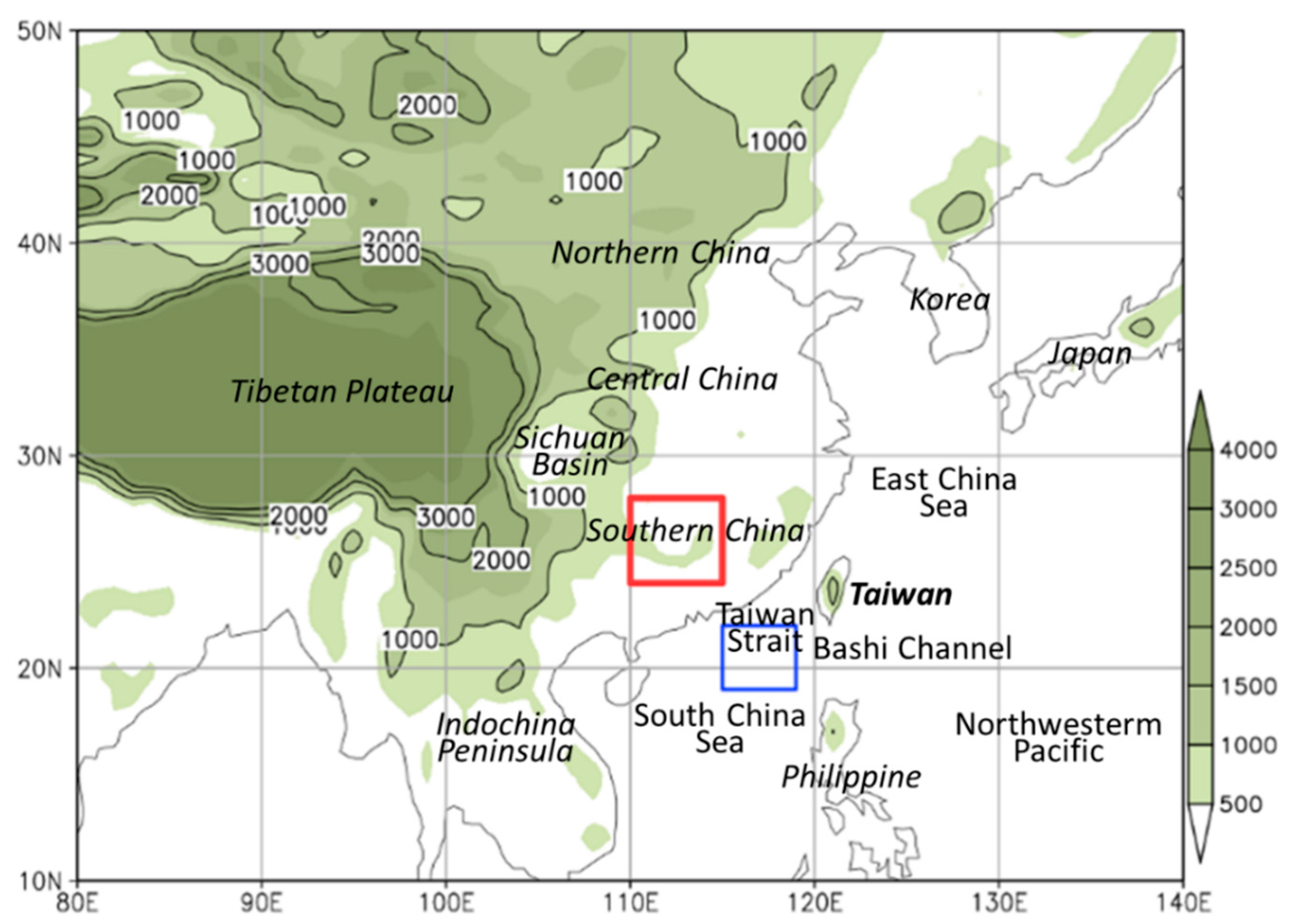
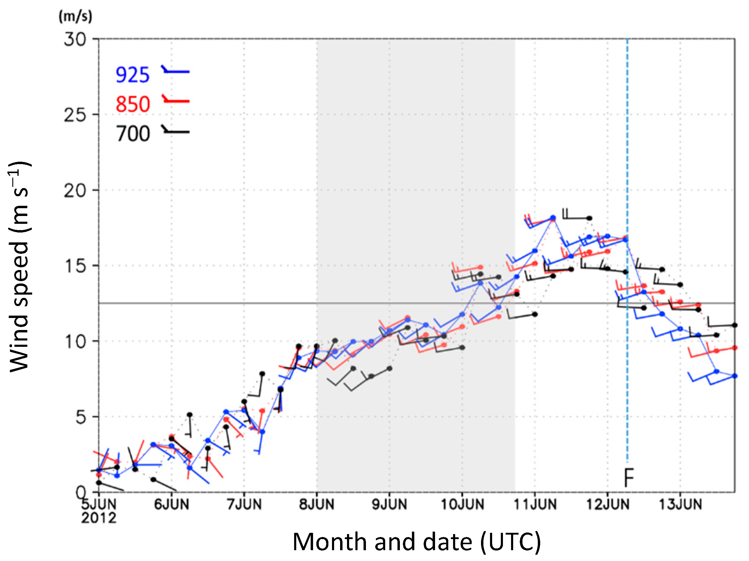
The analysis indicates that the heavy rainfall with such a long duration in Taiwan was due to a strong and persistent west-southwesterly LLJ that transported warm, moist, and unstable air from the upstream area, and then impinged on the topography of the island. The LLJ developed in response to an enhancement in the horizontal pressure (or geopotential height) gradient, when the pressure at low-levels fell significantly, by about 8 hPa, to the north of the jet in South China during a 66 h period on 8–10 June, but the STH to the southeast remained and did not retreat much.

(ii)

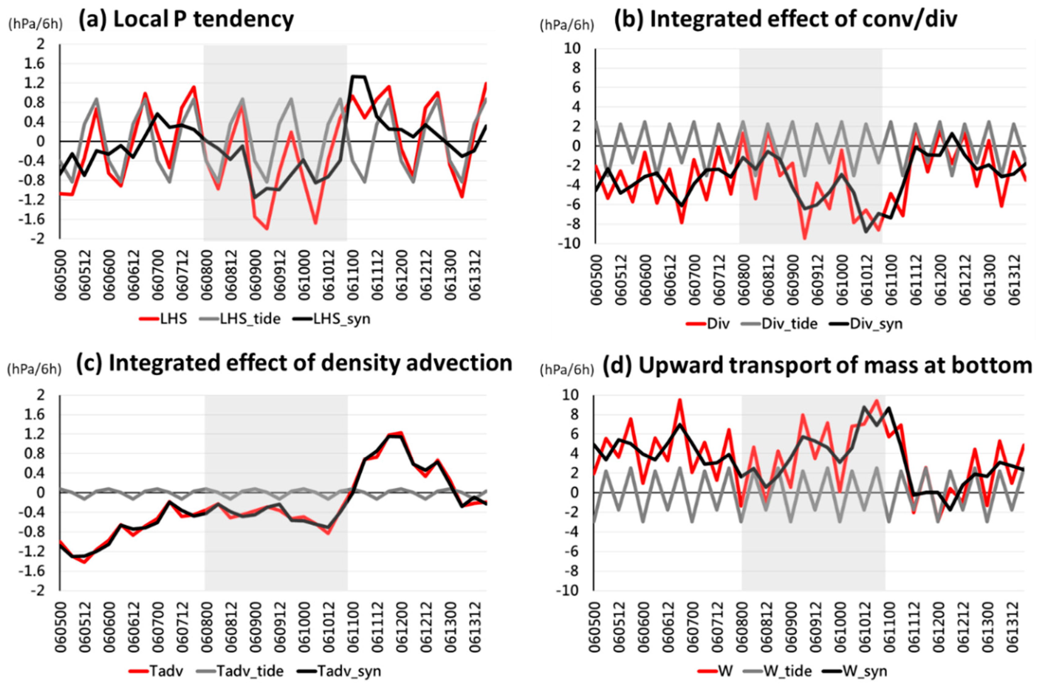
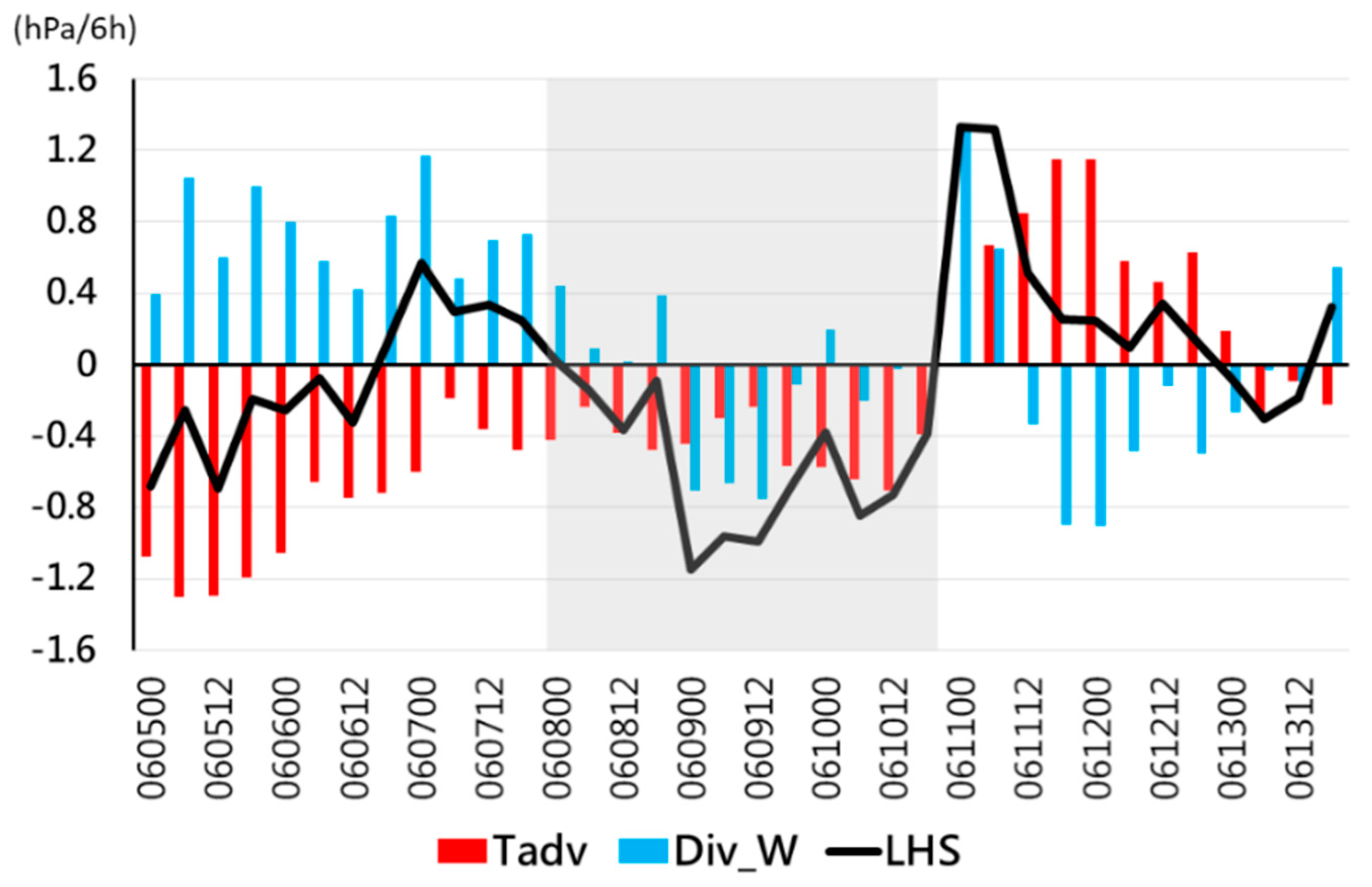
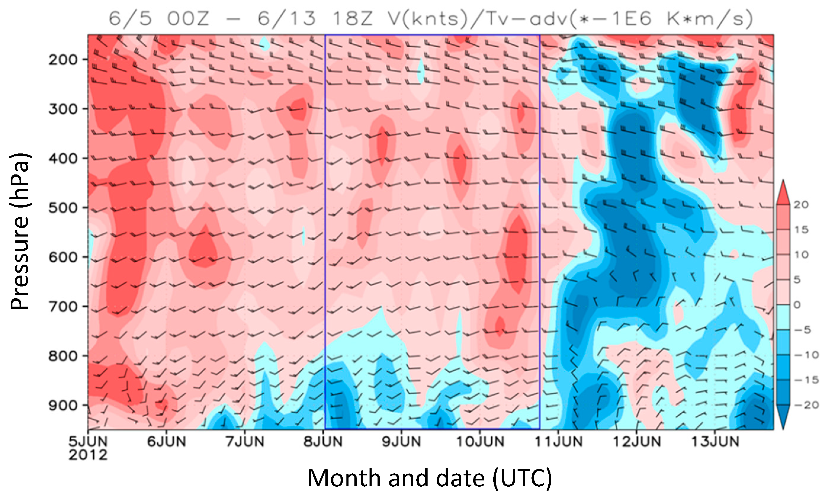
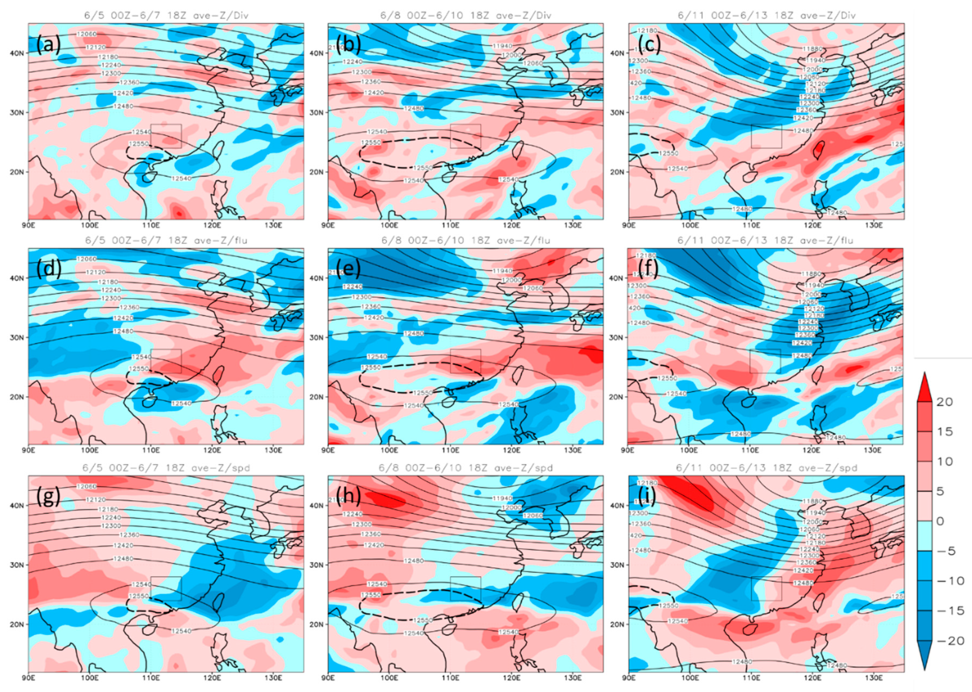
Through diagnosis using the pressure tendency equation, it is found that the persistent warm air advection through deep troposphere (mainly above 800 hPa) was a major contributor toward the pressure fall in South China during 8–10 June. From before the pressure fall period, a large-scale confluent pattern existed in China, and provided west-southwesterly flow and warm air advection in South China, thus transporting warmer and less dense air into the region from lower latitudes. While the effect of warm advection was even stronger during 5–7 June (before the fall period), it somewhat weakened during the fall period (8–10 June) but was still the main driver to pressure decrease on 8 and 10 June 2012.

(iii)

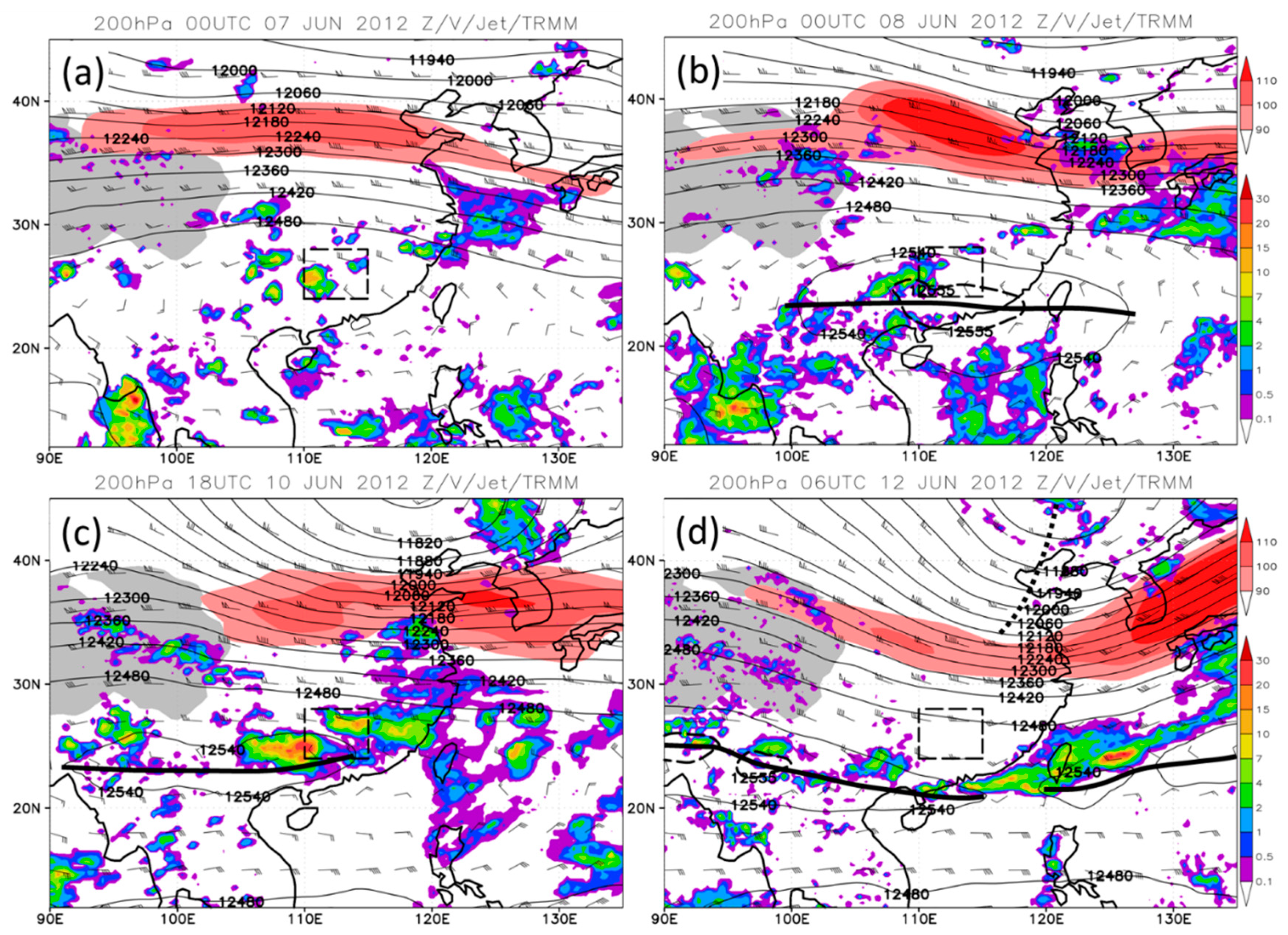
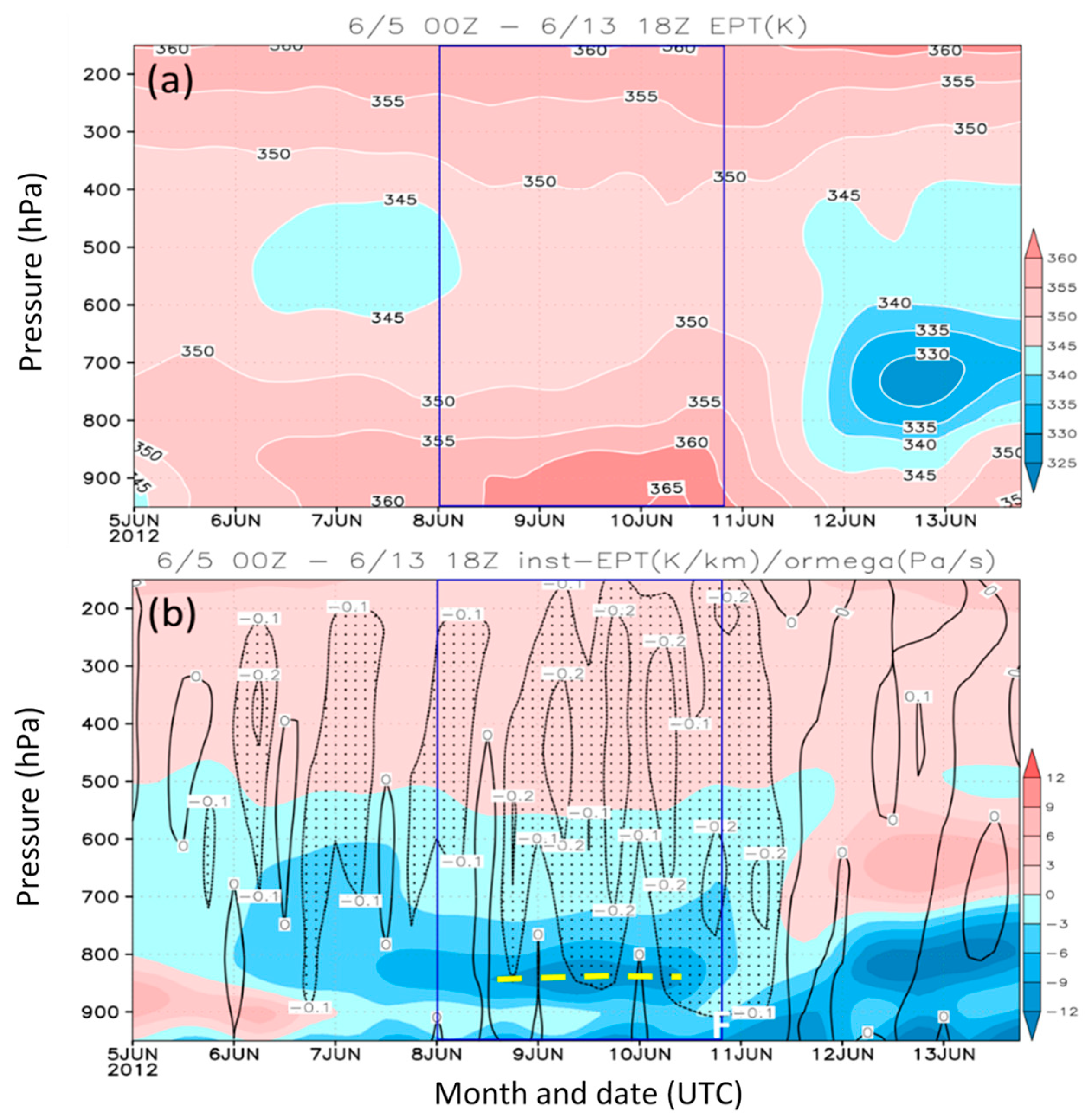
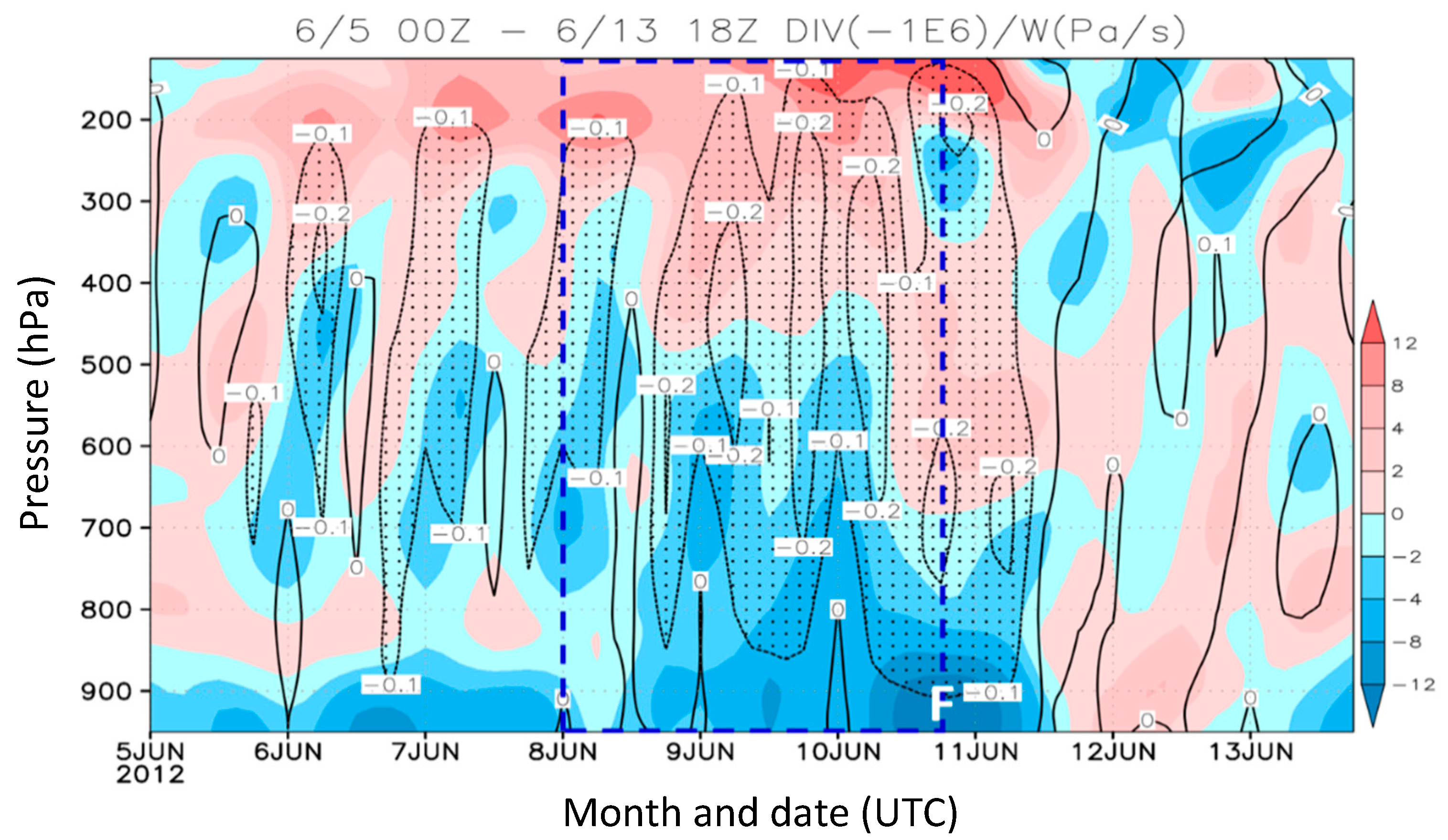
In the upper troposphere, the South Asian anticyclone had its center to the southwest of South China, and thus provided persistent upper-level divergence before and during the fall period (5–10 June), since South China was located in its northeastern quadrant with significant flow diffluence. During 5–10 June, the South Asian anticyclone and its associated divergence also strengthened, and with increased potential (or convective) instability and more vigorous convection development in South China, the divergence aloft was able to exceed low-level convergence to produce net mass outflow in the air column, and further at least cancel out the effect of rising motion (toward pressure rise) during 8–10 June. On 9 June, the two dynamic terms (convergence/divergence effect and vertical motion) in combination even contributed more than the warm air advection toward the pressure fall.

When the low-level pressure was falling in South China on 8 June, the southwesterly flow upstream of Taiwan just started to enhance (cf. Figure 5b). The synoptic conditions surrounding Taiwan was considered weak, but a surge in southwesterly flow, combined with the offshore land breeze, initiated several convective cells southwest of Taiwan near midnight that subsequently intensified and moved onshore to cause early morning rainfall [34]. After the pressure fall in South China and the development of the LLJ south of the front, heavy rainfall occurred in Taiwan three days in a row during 10–12 June (Figure 3). Of course, as the front approached northern Taiwan, two intense rainbands ahead of the front produced extreme rainfall (510 mm) in the Taipei Metropolitan Area roughly from 1200 UTC 11 to 0000 UTC 12 June [23], when the rainfall in southern Taiwan also continued (cf. Figure 3d). Interestingly, after the front moved south and across Taiwan, it retreated and moved north again during 13–14 June to cause another rainfall period in Taiwan [35]. Thus, this front lingered near Taiwan until 15 June 2012, and was certainly one of the most impactful and hazardous Mei-yu front to Taiwan in the past two decades.

References

1. Ding, Y.-H. Summer monsoon rainfalls in China. J. Meteor. Soc. Jpn. 1992, 70, 337–396. [Google Scholar] [CrossRef] [Green Version]
2. Chen, G.T.-J. Observational aspects of Mei-yu phenomena in subtropical China. J. Meteor. Soc. Jpn. 1983, 61, 306–312. [Google Scholar] [CrossRef] [Green Version]
3. Tao, S.; Chen, L. A review of recent research on the East Asian summer monsoon in China. In Monsoon Meteorology; Chang, C.-P., Krishnamurti, T.N., Eds.; Oxford University Press: Oxford, UK, 1987; pp. 60–92. [Google Scholar]
4. Lau, K.-M.; Yang, G.J.; Shen, S.H. Seasonal and intraseasonal climatology of summer monsoon rainfall over East Asia. Mon. Weather Rev. 1988, 116, 18–37. [Google Scholar] [CrossRef] [Green Version]
5. Chen, Y.-L. Some synoptic-scale aspects of surface fronts over southern China during TAMEX. Mon. Weather Rev. 1993, 121, 50–64. [Google Scholar] [CrossRef] [Green Version]
6. Chen, C.-S.; Chen, Y.-L. The Rainfall Characteristics of Taiwan. Mon. Weather Rev. 2003, 131, 1323–1341. [Google Scholar] [CrossRef]
7. Chen, G.T.-J.; Tsay, C.-Y. A synoptic case study of Mei-Yu near Taiwan. Papers Meteor. Res. 1978, 1, 25–36. [Google Scholar]
8. Chen, G.T.-J. On the moisture budget of a Mei-Yu system in southeastern Asia. Proc. Natl. Sci. Counc. 1979, 3, 24–32. [Google Scholar]
9. Chen, G.T.-J.; Chi, S.-S. On the meso-scale structure of Mei-Yu front in Taiwan. Atmos. Sci. 1978, 5, 35–47, (In Chinese with English Abstract). [Google Scholar]
10. Chen, G.T.-J.; Yu, C.-C. Role of Mei-Yu front and mesolow on the heavy rainfall events. Two cases in TAMEX Phase I (1986). Atmos. Sci. 1990, 18, 129–147, (In Chinese with English Abstract). [Google Scholar]
11. Li, J.; Chen, Y.-L.; Lee, W.-C. Analysis of a heavy rainfall event during TAMEX. Mon. Weather Rev. 1997, 125, 1060–1081. [Google Scholar] [CrossRef]
12. Chen, C.; Tao, W.-K.; Lin, P.-L.; Lai, G.S.; Tseng, S.-F.; Wang, T.-C.C. Wang. The intensification of the low-level jet during the development of mesoscale convective systems on a Mei-Yu front. Mon. Weather Rev. 1998, 126, 349–371. [Google Scholar] [CrossRef]
13. Chen, S.-J.; Kuo, Y.-H.; Wang, W.; Tao, Z.-Y.; Cuo, B. A modeling case study of heavy rainstorms along the Mei-Yu front. Mon. Weather Rev. 1998, 126, 2330–2351. [Google Scholar] [CrossRef]
14. Chen, S.-J.; Wang, W.; Lau, K.H.; Zhang, Q.H.; Chung, Y.S. Mesoscale convective systems along the Meiyu front in a numerical model. Meteor. Atmos. Phys. 2000, 75, 149–160. [Google Scholar] [CrossRef]
15. Chen, X.A.; Chen, Y.-L. 1995: Development of low-level jets during TAMEX. Mon. Weather Rev. 1995, 123, 1695–1719. [Google Scholar] [CrossRef] [Green Version]
16. Chen, G.T.-J.; Chang, C.-P. The structure and vorticity budget of an early summer monsoon trough (mei-yu) over southeastern China and Japan. Mon. Weather Rev. 1980, 108, 942–953. [Google Scholar] [CrossRef] [Green Version]
17. Chen, G.T.-J.; Wang, C.-C.; Liu, S.C.-S. Potential vorticity diagnostics of a Mei-yu front case. Mon. Weather Rev. 2003, 131, 2680–2696. [Google Scholar] [CrossRef]
18. Chen, G.T.-J.; Wang, C.-C.; Lin, L.-F. A diagnostic study of a retreating Mei-Yu front and the accompanying low-level jet formation and intensification. Mon. Weather Rev. 2006, 134, 874–896. [Google Scholar] [CrossRef]
19. Chen, G.T.-J.; Wang, C.-C.; Chang, S.-W. A diagnostic case study of Mei-yu frontogenesis and development of wavelike frontal disturbances in the subtropical environment. Mon. Weather Rev. 2008, 136, 41–61. [Google Scholar] [CrossRef]
20. Cho, H.-R.; Chen, G.T.-J. Mei-yu frontogenesis. J. Atmos. Sci. 1995, 52, 2109–2120. [Google Scholar] [CrossRef]
21. Chien, F.-C.; Hung, Y.-H. Composite and numerical studies of southwesterly flow in the Taiwan area during Mei-yu seasons. Atmos. Sci. 2010, 38, 237–267, (In Chinese with English Abstract). [Google Scholar]
22. Chen, G.T.-J. Large-scale circulations associated with the East Asian summer monsoon and the Mei-Yu over South China and Taiwan. J. Meteor. Soc. Jpn. 1994, 72, 959–983. [Google Scholar] [CrossRef] [Green Version]
23. Wang, C.-C.; Chiou, B.-K.; Chen, G.T.-J.; Kuo, H.-C.; Liu, C.-H. A numerical study of back-building process in a quasistationary rainband with extreme rainfall over northern Taiwan during 11–12 June 2012. Atmos. Chem. Phys. 2016, 16, 12359–12382. [Google Scholar] [CrossRef] [Green Version]
24. Chen, Y.-L.; Chu, Y.-J.; Chen, C.-S.; Tu, C.-C.; Teng, J.-H.; Lin, P.-L. Analysis and simulations of a heavy rainfall event over northern Taiwan during 11–12 June 2012. Mon. Weather Rev. 2018, 146, 2697–2715. [Google Scholar] [CrossRef]
25. Dee, D.P.; Uppala, S.M.; Simmons, A.J.; Berrisford, P.; Poli, P.; Kobayashi, S.; Andrae, U.; Balmaseda, M.A.; Balsamo, G.; Bauer, D.P.; et al. The ERA-Interim reanalysis: Configuration and performance of the data assimilation system. Quart. J. Roy. Meteor. Soc. 2011, 137, 553–597. [Google Scholar] [CrossRef]
26. Huffman, G.J.; Adler, R.F.; Bolvin, D.T.; Gu, G.; Nelkin, E.J.; Bowman, K.P.; Hong, Y.; Stocker, E.F.; Wolff, D.B. The TRMM Multisatellite Precipitation Analysis (TMPA): Quasi-global, multiyear, combined-Sensor precipitation estimates at fine scales. J. Hydrometeorl. 2007, 8, 38–55. [Google Scholar] [CrossRef]
27. Hsu, J. ARMTS up and running in Taiwan. Väisälä News 1998, 146, 24–26. [Google Scholar]
28. Gettelman, A.; de F Forster, P.M. A climatology of the tropical tropopause layer. J. Meteor. Soc. Jpn. 2002, 80, 911–924. [Google Scholar] [CrossRef] [Green Version]
29. Fueglistaler, S.; Dessler, A.E.; Dunkerton, T.J.; Folkins, I.; Fu, Q.; Mote, P.W. Tropical tropopause layer. Rev. Geophys. 2009, 47, RG1004. [Google Scholar] [CrossRef]
30. Chen, Y.-L.; Li, J. Large-scale conditions favorable for the development of heavy rainfall during TAMEX. Mon. Weather Rev. 1995, 123, 2978–3002. [Google Scholar] [CrossRef] [Green Version]
31. Chen, C.-S.; Chen, W.-C.; Chen, Y.-L.; Lin, P.-L.; Lai, H.-C. Investigation of orographic effects on two heavy rainfall events over southwestern Taiwan during the Mei-yu season. Atmos. Res. 2005, 73, 101–130. [Google Scholar] [CrossRef]
32. Wang, C.-C.; Hsu, J.C.-S.; Chen, G.T.-J.; Lee, D.-I. A study of two propagating heavy-rainfall episodes near Taiwan during SoWMEX/TiMREX IOP-8 in June 2008. Part I: Synoptic evolution, episode propagation, and model control simulation. Mon. Weather Rev. 2014, 142, 2619–2643. [Google Scholar] [CrossRef]
33. Wang, C.-C.; Hsu, J.C.-S.; Chen, G.T.-J.; Lee, D.-I. A study of two propagating heavy-rainfall episodes near Taiwan during SoWMEX/TiMREX IOP-8 in June 2008. Part II: Sensitivity tests on the roles of synoptic conditions and topographic effects. Mon. Weather Rev. 2014, 142, 2644–2664. [Google Scholar] [CrossRef]
34. Wang, C.-C.; Chen, G.T.-J.; Ngai, C.-H.; Tsuboki, K. Case study of a morning convective rainfall event over southwestern Taiwan in the Mei-yu season under weak synoptic conditions. J. Meteor. Soc. Jpn. 2018, 96, 461–484. [Google Scholar] [CrossRef] [Green Version]
35. Wang, C.-C.; Chen, G.T.-J.; Ho, K.-H. A diagnostic case study of mei-yu frontal retreat and associated low development near Taiwan. Mon. Weather Rev. 2016, 144, 2327–2349. [Google Scholar] [CrossRef]
Figure 1. A map and topography (m, color) in East Asia. The red box (24°–28° N, 110°–115° E) shows the region to compute pressure fall and its related diagnosis, and the blue box (19°–22° N, 115°–119° E) is the region to compute mean flow upstream of Taiwan.
Atmosphere 12 01255 g001
Figure 2. The JMA surface weather map at (a) 0000 UTC 10, (b) 1800 UTC 10, (c) 1200 UTC 11, and (d) 0600 UTC 12 June 2012, respectively. The Mei-yu front is depicted as stationary.
Atmosphere 12 01255 g002
Figure 3. Daily rainfall distribution (mm; 0000-2400 UTC) from the gauge network in Taiwan on (a) 9, (b) 10, (c) 11, (d) 12, and (e) 13 June 2012. The location and value of daily maximum in each panel are marked.
Atmosphere 12 01255 g003
Figure 4. The time series of surface pressure (hPa) in ERA-Interim data, averaged inside the red box in Figure 1, in South China from 0000 UTC 5 to 1800 UTC 13 June 2012. The shading in gray indicates the period of most significant pressure fall (by 7.8 hPa in 66 h, from 0000 UTC 8 to 1800 UTC 10 June).
Atmosphere 12 01255 g004
Figure 5. The geopotential height (gpm, contours, every 10 gpm), horizontal winds (barbs, full barb = 10 kt), equivalent potential temperature (θe, K, color), and the location of LLJ exceeding 12.5 m s1 (stippled) at 850 hPa at (a) 0000 UTC 7, (b) 0000 UTC 8, (c) 1800 UTC 10, and (d) 0600 UTC 12 June 2012 in the ERA-Interim analysis. The ridge (thick solid line), trough (dotted line), and surface frontal location (in JMA charts; blue dashed line) are marked. Gray shades indicate the topography higher than 1500 m, and the box for average in South China is also plotted (dashed box).
Atmosphere 12 01255 g005
Figure 6. The geopotential height (gpm, contours, every 30 gpm), horizontal winds (barbs, full barb = 10 kt), virtual temperature (θv, °C, red dotted isotherms with blue labels), and relative vorticity (10−5 s−1, color, scale to the right) at 500 hPa at (a) 0000 UTC 7, (b) 0000 UTC 8, (c) 1800 UTC 10, and (d) 0600 UTC 12 June 2012 in the ERA-Interim analysis. The ridge (thick solid line) and trough (dotted line) are marked where needed, and the box for average in South China is also plotted (dashed box).
Atmosphere 12 01255 g006
Figure 7. The geopotential height (gpm, contours, every 60 gpm), horizontal winds (barbs, full barb = 10 kt), and upper-level jet in excess of 90 kts (color, scale to upper right) at 200 hPa in the ERA-Interim analysis, overlaid with TRMM rainrate (mm h−1, color, scale to lower right) at (a) 0000 UTC 7, (b) 0000 UTC 8, (c) 1800 UTC 10, and (d) 0600 UTC 12 June 2012. The ridge (thick solid line) and trough (dotted line) are marked where needed. Gray shades indicate the topography higher than 3000 m, and the box for average in South China is also plotted (dashed box).
Atmosphere 12 01255 g007
Figure 8. As in Figure 4, but showing the time series of geopotential height (gpm), averaged inside the red box in Figure 1 in South China at (a) 925 (blue), 850 (red), and 700 hPa (black), and (b) 500 (blue), 300 (red), and 200 hPa (black), from 0000 UTC 5 to 1800 UTC 13 June 2012.
Atmosphere 12 01255 g008
Figure 9. The time series of horizontal winds (m s−1, barbs, full barb = 10 m s−1) in the ERA-Interim analysis at 925 (blue), 850 (red), and 700 hPa (black), respectively, averaged inside the blue box in Figure 1 in the upstream area of Taiwan, from 0000 UTC 5 to 1800 UTC 13 June 2012. The symbol “F” marks the time when the surface front reached northern Taiwan.
Atmosphere 12 01255 g009
Figure 10. (a) The low-level pressure tendency in South China (computed for the red box in Figure 1), and its three forcing terms of (b) column-integrated convergence/divergence, (c) column-integrated density (thermal) advection, and (d) mass transport by vertical motion (all in hPa per 6 h), from 0000 UTC 5 to 1800 UTC 13 June 2012. For each term, the original time series (red), its diurnal (or semi-diurnal) component (gray), and the synoptic signals (black, = red minus gray) are shown. The time in the horizontal axis is given in the format of “mmddtt” for month, date, and time (h in UTC).
Atmosphere 12 01255 g010
Figure 11. As in Figure 10, but showing the synoptic-scale signals of the pressure tendency (black), column-integrated density (thermal) advection (red bars), and the combined dynamic effect (blue bars, i.e., column-integrated convergence/divergence plus the mass transport by vertical motion. All units are in hPa per 6 h.
Atmosphere 12 01255 g011
Figure 12. Time-height cross section of virtual temperature advection (color, 10−6 K s−1) in South China from the ERA-Interim data, averaged inside the red box in Figure 1, from 0000 UTC 5 to 1800 UTC 13 June 2012. The thin blue box marks the pressure fall period in South China.
Atmosphere 12 01255 g012
Figure 13. As in Figure 12, but showing the section of (a) equivalent potential temperature (θe, K, color with white isotherms very 5 K) and (b) potential stability (∂θe/z, K km−1, color) and rising motion in ω (= dp/dt, Pa s−1, contour every 0.1 Pa s−1 and stippled for ω < −0.1 Pa s−1) in South China (red box in Figure 1), from 0000 UTC 5 to 1800 UTC 13 June 2012. The yellow dashed line in (b) marks the most unstable level.
Atmosphere 12 01255 g013
Figure 14. As in Figure 12b, but showing the divergence (D, color, 10−6 s−1) in South China, in addition to the rising motion in ω (Pa s−1, stippled for ω < −0.1 Pa s−1).
Atmosphere 12 01255 g014
Figure 15. Time-averaged geopotential height (gpm, contours, every 60 gpm, additional dashed contours where needed) and divergence (D, color, 10−6 s−1) from the ERA-Interim data at 200 hPa over (a) 0000 UTC 5 to 1800 UTC 7, (b) 0000 UTC 8 to 1800 UTC 10, and (c) 0000 UTC 11 to 1800 UTC 13 June 2012, respectively. (df) As in (ac) but for diffluence component of D. (gi) As in (ac) but for the speed divergence/convergence of D. The box for average in South China is also plotted.
Atmosphere 12 01255 g015