Abstract
Parametrization of radiation transfer through clouds is an important factor in the ability of Numerical Weather Prediction models to correctly describe the weather evolution. Here we present a practical parameterization of both liquid droplets and ice optical properties in the longwave and shortwave radiation. An advanced spectral averaging method is used to calculate the extinction coefficient, single scattering albedo, forward scattered fraction and asymmetry factor (βext, ϖ, f, g), taking into account the nonlinear effects of light attenuation in the spectral averaging. An ensemble of particle size distributions was used for the ice optical properties calculations, which enables the effective size range to be extended up to 570 μm and thus be applicable for larger hydrometeor categories such as snow, graupel, and rain. The new parameterization was applied both in the COSMO limited-area model and in ICON global model and was evaluated by using the COSMO model to simulate stratiform ice and water clouds. Numerical weather prediction models usually determine the asymmetry factor as a function of effective size. For the first time in an operational numerical weather prediction (NWP) model, the asymmetry factor is parametrized as a function of aspect ratio. The method is generalized and is available on-line to be readily applied to any optical properties dataset and spectral intervals of a wide range of radiation transfer models and applications.
Keywords:
clouds; optical properties; radiative transfer; ice particles; water droplets; NWP; climate; modeling 1. Introduction
Clouds have the main influence on the radiative fluxes in the atmosphere and on the entire atmospheric energy budget. The increase of aerosol number concentration can increase cloud droplets number concentration and retardation in their growth [1]. This effect may suppress drizzle and reduce the cloud droplet size, which would cause an increase in cloud albedo (cooling effect) [2,3]. Cloud radiative feedback (CRF), particularly of water clouds, is the dominant uncertainty for climate sensitivity [4,5].
The main goal of this work is to re-calculate the optical properties of both water droplets and ice particles enabling a simple implementation in both numerical weather prediction (NWP) and climate models (CLM). The benefit is measured by the non-hydrostatic compressible COSMO model (http://www.cosmo-model.org).
1.1. Hydrometeors Optical Properties
1.1.1. Ice Particles
The optical properties of hydrometeors calculated in radiative transfer schemes are highly important in any NWP and CLM. Usually, there is a gap between the data available in the literature based on in situ measurements and numerical methods and those used in operational models. The common difficulties are the different wavelength intervals used and the high variability in particle-size distributions (PSDs) and shape [6]. Cirrus clouds containing pure ice crystals cover roughly 20%–40% of the earth’s troposphere and are of great impact on the earth’s energy budget [6,7,8]. These clouds have a warming effect at the top of the atmosphere of approximately 5 W/m2 in the global annual average that was confirmed by numerous modeling and observational studies [9,10]. The optical properties of ice hydrometeors were for many years one of the unsolved problems of climate models. One of the main reasons for this difficulty is the various shapes of ice crystals such as plates, columns, bullet rosettes, and aggregates of these. The size range of ice particles is also much larger compared to water droplets [11]. As to date, there is no general analytical solution for the scattering and absorption of non-spherical ice particles. Nevertheless, ray scattering calculations and other models based on geometric optics can be used to calculate the single scattering optical properties of ice particles with a large range of size parameter in clouds [12,13]. Fu and Liou (1993) [11] followed the work of Takano and Liou (1989) [14] and used a light scattering program including a geometric ray-tracing program to calculate the single-particle optical properties. The mass extinction coefficient, single scattering albedo, and expansion coefficients of the phase function were calculated for 11 observed PSDs (references can be found in Fu and Liou, 1993) [11]. These authors parametrized the optical properties for 18 broadband intervals as a function of ice water content (IWC) and mean effective size, defined as:
Where D and L are the randomly oriented hexagonal particles’ width and length respectively and n(L) is the PSD. The single-particle aspect ratio D/L used here was based on observational data [15]:
Since most atmospheric ice particles are much larger than most of the solar radiation wavelengths, geometric optics approximations are sufficiently accurate to model ice particles and radiation interactions [16].
The generalized effective size () is more suitable than for ice optical properties parametrizations. This quantity is the ratio between the volume and the statistically averaged projected area () of the randomly oriented needle particle (see Equations 2.3, 3.10, and 3.11 in Fu, 1996) [11]:
The generalized effective size () can be related to the effective radius using the formula:
The size parameter (α) is defined by the particle size to wavelength ratio:
where λ is the wavelength, rva = 3V/3A is the equivalent radius for a non-spherical particle by conserving both its volume (V) and projected area (A) [17]. Ice crystals have a large variety of shapes, sizes, and complexity, which depends mainly on temperature and humidity. The volume extinction coefficient and single scattering albedo for randomly oriented hexagonal ice columns can be parameterized by the generalized effective size and the IWC [15,17]. These parametrizations can be well applied to other ice particle shapes since the IWC, along with , conserves both the projected area and volume of non-spherical ice particles which largely determine the ice particle extinction and absorption [15].
As for the asymmetry factor, ray scattering simulations for many types of ice crystals showed that it is less dependent on size rather on the aspect ratio D/L [16,18] or more generally, the effective aspect ratio [18]:
Fu (2007) [18] also showed that the asymmetry factor bulk parameterization based on the aspect ratio (AR) is less sensitive to the detailed ice shape.
Fu (1996) [15] calculated the optical properties of cirrus clouds for 28 PSDs. His work was based on both conventional geometric ray-tracing for large particles with a size parameter greater than 200 and improved geometric ray tracing by Yang and Liou (1995) [19] for smaller particles. These PSDs were taken from several in situ aircraft observation campaigns in mid-latitudes and tropical regions. The optical properties were parameterized as a function of and IWC, which for hexagonal particles is:
where ρice is the bulk ice density (0.917 g·cm−3). The parametrizations for volume extinction coefficient and single-scattering albedo were adequate for various randomly-oriented non-spherical particles although the randomly-oriented hexagonal particles were assumed. Note that horizontally oriented ice particles appear infrequently: ~ 12% in mid-latitude and near zero in the tropics (see Table 3 in Thorsen and Fu 2015 [20]).
The parameterization of the asymmetry factor as a function of is due to the dependence of the aspect ratio on the ice particle size used (i.e., Equation (2)), which might not be generally valid [18]. In infrared (IR) wavelengths, an ice particle’s absorption is the dominant effect but one cannot neglect the scattering effect [21]. Fu et al. (1998) [17] used a linear combination of Mie theory, anomalous diffraction theory (ADT), and the geometric optics method (GOM) to calculate the IR radiative properties of ice crystals and to address the wide range of size parameter. The finite-difference time-domain (FDTD) method [22] was used as a reference calculation. These authors used the same 28 PSDs as used by Fu (1996) [15] dividing the distributions into 38 discrete size bins in the range of Lmin = 1 μm to Lmax = 3 mm. The bulk optical properties were parameterized as a function of IWC and for wavelengths in the range between 3.969 μm and 100 μm. Compared to the reference results, the averaged relative error was only ~2% for the emissivity of cirrus clouds.
Yang et al. (2000) [7] published their work on the single scattering optical properties of six ice crystals habits that are usually found in in situ measurements (plate, columns, hollow column, planar and spatial bullet rosettes, and aggregates) and spectral bands in the range 0.2 μm–5 μm. They used GOM and FDTD to calculate the extinction and absorption coefficients, and the asymmetry factor and forward peak of the phase function (the latter is only significant for short wave intervals), which were parameterized as a function of effective size. In their study, they fitted the diameter of equivalent area DA and the diameter of equivalent volume Dv in terms of the maximum dimension Dmax for each crystal shape where the Dmax/Deff ratio depends on the ice particle habit.
Baum et al. (2005) [23] have investigated the bulk properties of ice particles using PSDs data taken from in situ field campaigns in five different locations over the tropics and mid-latitudes namely FIRE-I, FIRE-II, ARM, TRMM, and CRYSTAL FACE field campaigns (see their Table 1 therein). There were 1117 PSDs parameterized by fitting to a gamma distribution of the form:
The bulk characteristics of IWC and the median mass diameter Dm were represented analytically as a function of μ Λ and . To overcome the differences between calculated and in situ measured IWC for all field experiments, the size range was divided into parts and for each, a mixture of habits (droxtals, bullet rosettes, solid columns, and aggregates) was assumed. Baum et al. (2011) [24] calculated the bulk optical properties of ice cloud in the shortwave regime based on 12 thousand PSDs from both northern and southern hemisphere field campaigns containing nine habits with different roughness levels. From the comparison between their models and cloud-aerosol lidar with orthogonal polarization (CALIOP) data, they concluded that rough surface particles are best for modeling a mixture of habits that usually exist in frozen clouds. The wavelengths used were in the range of 0.4–2.24 μm in a later work [25], they expanded their results for 445 discrete wavelengths in the range 0.2–100 μm using the Yang et al. (2013) [12] data set. The latter used the Amsterdam discrete dipole approximation (ADDA), the T-matrix, and the improved geometric optics (IGOM) methods in the range of 0.4–100 μm. They included 11 ice particle habits in the size range of 2 μm to 10 mm divided into 189 size bins with three roughness levels. This publication provided the most up to date data library for the widest range of shapes, sizes, and wavelengths.
As the main goal of this work was to implement an efficient, simple, and fast scheme for NWP and CLM models, the single-particle data by Fu (1996) [15] and Fu et al. (1998) [17] was chosen as the base of our parametrizations for ice optical properties.
1.1.2. Water Droplets
The effective radius of water droplets is defined as the ratio of the third to the second moments of a droplet size distribution [26]:
There are large uncertainties in simulated cloud cover, liquid water content (LWC), droplets size distributions, and from the NWP and CLM [27]. On top of these are the uncertainties in the optical properties of these hydrometeors namely the volume extinction coefficient (βext), asymmetry factor (g), and single scattering albedo () at each cloud layer. Fortunately, LWC and are usually enough for a reasonable approximation of the cloud’s optical properties even without knowing the exact particle size distributions (PSD) in the cloud [28]. Based on the Delta-Edington approximation for vertically inhomogeneous atmosphere [29], Slingo and Schrecker (1982, SS82 hereafter) [30] calculated a 24-band parametrization for g, , and βext as a function of LWC and in the shortwave range of 0.25–4 μm. Slingo (1989) [31] used SS82 parametrizations and further developed the equations for the transmissivity, reflectivity, and absorptivity. These parametrizations were implemented into Helios, the UK Met Office global circulation model (GCM) radiation subroutine that was later replaced by the Edwards and Slingo (1996) [32] scheme. This author also made comparisons with Stephens (1984) [33] parametrization vs. aircraft observations and showed positive results. Hu and Stamnes (1993) (hereafter HS93) [28] published their work on liquid cloud optical properties based on Mie calculations. They expanded the spectral range to the longwave (LW) compared to previous works which mainly addressed the short wave (SW) of the solar radiation. Their work included computation of g, and for 74 wavelengths between 0.29–150 μm and parametrized them for three droplet size ranges: 2.5–12 µm, 12.5–30 µm, and 30–60 µm. The parametrization was defined by non-linear square fitting to the exponential functions:
where , are the fitting coefficients. HS93 also showed that for a fixed effective radius, the optical properties change only slightly (1%–2%) even under large variations in the PSD width, shape, skewness, and modality (number of modes in the distribution). Even changing the PSD from lognormal to a generalized gamma distribution with different widths showed only up to 8% differences in the optical properties of the clouds. The parameterization used was as accurate as exact Mie calculations but three orders of magnitudes faster. Later, Lindner and Li (2000) [34] calculated cloud droplets’ optical properties for 36 wavelengths in the infrared spectrum between 4 µm and 1000 μm. Based on the exact Mie calculation, they used the least square fitting technique for the bulk optical properties for particles in the size range of 2–40 μm. While HS93 fitted the optical properties to exponential functions and used three size bins, Lindner and Li (2000) [34] defined a single parametrization for the whole size range and used rational functions of the form:
Since HS93 includes both SW and LW spectral ranges, we adopted the HS93 fitting functions but used a single parametrization for the whole size range.
2. Optical Properties Parametrization
2.1. Ice Particles
Raw data for the single-particle extinction and scattering cross-sections (σext, σsca), asymmetry factor (gp), and the forward scattering δ function peak (fδ) were taken from Fu (1996) [15] and Fu et al. (1998) [17]. In this work, all particles were assumed randomly oriented hexagons particles of length L and diameter D, which are related in Equation (2). Although a more recent state-of-the-art work on a wider range of habits was available, most notably by Yang et al. (2013) [12], there were two main reasons for our choice. First, the parametrizations of the optical properties in terms of IWC, generalized effective sizes, and mean aspect ratio could be applied to ice clouds containing ice particles with complicated shapes [15,17,18] by conserving ice particle ice volume, projected area, and mean aspect ratio. For example, as shown in Fu (2007) [18], for the SW, this parameterization well reproduced the asymmetry factors of complicated ice particles such as bullet rosettes, aggregates with rough surfaces, and fractal crystals and agreed well with observations. Second, the diagnosis of the habit-mixture composition of ice particles at each grid-box containing ice was not straightforward while the computational cost could be high. Although scientifically reasoned, it was impractical for present-day operational numerical weather prediction models.
Further discussion on the bulk optical properties of cirrus clouds, shape consideration, and their effects on climate models can be found in Baran et al. (2014, 2016) [35,36].
For SW radiation, L and D were discretized in 30 non-equidistant sizes from 8.75 to 3100 µm [15]. The data covered 200 wavelengths from 0.21 to 5 µm, which we used for SW. For the thermal infrared range (LW) the particle axis ratios were the same, but the data set was extended by 10 smaller particle sizes down to L = 2 µm. There were 36 wavelengths from 3.969 µm to 100 µm [17].
The equations for the transition from single-particle data to cloud optical properties were:
where , are the volume extinction and scattering coefficients, ω is the single scattering albedo, g is the asymmetry factor, and fd is the delta fraction (gp and fδ are the single-particle asymmetry factor and delta fraction respectively). is the mass extinction coefficient. An ensemble of particles was defined with a PSD, which was assumed to follow a four-parameter modified gamma distribution MGD [37]:
where is the scale parameter and μ, υ, Λ control the shape of the distribution, is the size distribution ith moment, and is the mean particle length. A simpler gamma distribution was obtained by setting υ = 1 hence:
We composed our PSD ensemble by a systematic variation of the PSD parameters within a wide range. We changed in the range of 5–3000 μm in 500 logarithmically equidistant steps, while μ was changed from 0 to 14 in steps of 1. Λ was computed from and μ using (2.10) resulting in 7500 PSDs. Applying the described ensemble of PSDs into Equation (3) with D(L) from Equation (2), resulted in a range of 5–600 µm in the generalized effective size (). The aspect ratio AR was computed using Formula 5 and results were in the range of 0.22–1.0. In the NWP model (i.e., COSMO), and AR could be evaluated from the mass-size relation used by the cloud microphysics scheme, for example, m = αLb where m is the particle mass. See Smith et al. (2016) [38] for further discussion on the issue.
The technique of spectral averaging over wide bands, representative for typical ice water paths (IWP) encountered in NWP-models, depends on the parameter one desires to compute. For , the physically appropriate definition equation for spectral averaging would be as follows:
where is the wavelength, is the Planck’s function for an appropriate radiation source temperature, is a certain probability density function (PDF) of the vertical model layer thickness , is the IWC PDF, and IWC Δz is the ice water path (IWP). Nevertheless, Equation (26) was not practical because of the unclear definition of the “mean” ice water path . Instead, we propose to first separately average over wavelength and then average the result over and . The first step is:
For numerical quadrature (integration), we employed the trapezoidal rule on the non-equidistant original wavelength discretization of the single-particle scattering data. The second step based on this result is:
For quadrature, we used an equidistant discretization of IWC and Δz with constant increments ΔIWC and Δ(Δz) and also employed the trapezoidal rule:
The IWC PDF was defined as a triangular function in the interval:
where:
The level thickness function was defined as a uniform distribution in the range [ΔZmin. ΔZmax]:
where:
For our purposes = 1 gm−3, ΔIWC = 0.01 gm−3, ΔZmin = 100 m, ΔZmax = 600 m and Δ(Δz) = 10 m were chosen. For the single scattering albedo calculation we used the same numerical method as in (27) but the following formula:
The same is done for the asymmetry factor using the formula:
The formula for the forward peak is similar to (34).
We parametrized as a function of and by fitting rational functions division using the Padé approximation form:
where can be or and are fitting coefficients. This approximation is a common practice for these parametrizations [39] and requires a non-linear fitting algorithm like Levenberg-Marquardt. It is very flexible and can reproduce nearly any asymptotic behavior if N and M are chosen adequately. If, an asymptotic convergence to a constant for results. If , the function converges to 0. We tried many other fitting functions, also the ones available in previous publications, but the mentioned method led to the best results for all spectral intervals. For , we chose, for and , we defined while for we put. The reasoning for choosing the AR and not as the fitting parameter for both the asymmetry factor and delta function is thoroughly discussed by Fu (2007) [18]. For simplicity reasons we used also for the LW intervals since scattering is less important in the thermal spectrum and we assumed the radiation model would not be sensitive to the difference between and . Another reason for choosing was the lack of confidence in the extrapolation of the fitting functions of for particles larger than the largest calculated point ( in the LW regime. Unlike the asymmetry factor, both the extinction coefficient and the single scattering albedo fits can be safely extrapolated to particles larger than that in the entire spectral range. These parametrization fits were applied to the eight spectral bands of the COSMO model radiation scheme (Ritter and Geleyn, 1992—RG92 thereafter) [40]. An example of the parametrization fit for three spectral intervals: 0.25–0.7 μm (SW), 1.53–4.64 μm (SW) and 20–104 μm (LW) can be seen in Figure 1. We could see had an exponential decrease as a function of size in the SW, while in the LW intervals, a peak was seen around an effective size of 30 μm. A single scattering albedo of 1 for the entire range of particle sizes in the 0.25–0.7 μm (SW) interval meant that 100% of extinction was due to scattering. For longer wavelengths, this amount was decreasing adding more absorption contribution to the extinction. A similar peak in single scattering albedo was seen in the LW as was seen in the curve. As for the asymmetry factor, we could see an almost linear decrease as a function AR which was a surprisingly simple description for an ensemble of 7500 PDFs and a very large range of particle sizes. Contours of the optical properties parametrizations can be seen in Figure 2. The extinction efficiency in this plot is calculated using the relation:
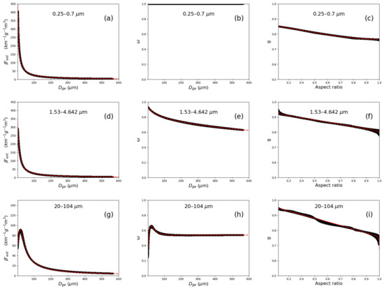
Figure 1.
Parametrizations for (a,d,g), single scattering albedo (b,e,h), and asymmetry factor (c,f,i) of hexagonal ice particles. The upper, middle, and lower rows refer to wavelengths of 0.25–0.7 μm (SW) (a–c), 1.53–4.64 µm (SW) (d–f), and 20–104 μm (LW) (g–i), intervals respectively. The black line is composed of 7500 individual points, each represents a different particle-size distribution (PSD), and the red dashed line denotes the parametrization fit model. Notice the scale difference between (a,d,g).
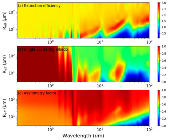
Figure 2.
Contours of the (a) extinction efficiency, (b) single-scattering albedo, and (c) asymmetry factor of hexagonal ice particles as a function of effective radius and wavelength. The extinction efficiency is calculated using Equation (36).
The asymmetry factor presented in Figure 1 and Figure 2 were calculated for particles with smooth surfaces, where the forward scattered peak (delta fraction) was large because of the plane-parallel surfaces of the ice particles. However, real particles might have rough surfaces, where there is more diffuse scattering. Therefore, an asymmetry factor for rough surfaces was defined as [18]:
The results for and for the 0.25–0.7 µm and 1.53–4.64 µm spectral intervals are shown in Figure 3. We note here that was calculated following the same methodology applied for but using Equation (37). Although the differences between and were less than + 3% for the spectral intervals selected in this work, a small but important difference will be presented in the results section. We assumed here that the scattering in the LW was less important (although not negligible) and that uncertainties in its asymmetry factor would not significantly affect the radiative energy budget.
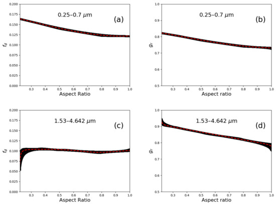
Figure 3.
Parametrizations for delta fraction (a,c) and rough surface particle asymmetry factor (b,d). The upper and lower rows refer to wavelengths of 0.25–0.7 µm (a,b) and 1.53–4.642 µm (c,d) intervals respectively. The black line is composed of 7500 individual points, each represents a different PSD, and the red dashed line denotes the parametrization fit model.
In the original RG92-formulation, the scattering phase function is approximated by the so-called δ-Eddington approximation, which is a sum of a general two-term Legendre-polynomial expansion of the phase function plus a delta-forward peak, weighted by the forward scattered fraction [41]. This approximation was “tuned” to the original phase function by matching , which is the first moment of the phase function, and by requiring that , which follows from the matching of the second moment of the phase function with that of the Greenstein function.
For ice particles in the visible spectral range, we changed the RG92 formulation in a way that was an independent free parameter [18]:
For rough surfaces particles and:
For smooth surfaces, for which a directly transmitted fraction is added (plane-parallel surfaces). We did, however, limit f so that it could not be larger than.
2.2. Liquid Droplets
For the quasi-spherical water droplets parametrization, we defined the effective radius as:
This definition is motivated by the large-size limit where is directly proportional to:
Where the geometric cross-section of a spherical droplet, LWC is the liquid water content, are the number concentration and bulk density of water, respectively. The constant coefficients depend on the constant mass-size-relation parameters and the size distribution parameters.
Based on Mie calculations performed by HS93 with a few typing corrections in the original tables, and using the spectral averaging technique described in the previous section, we applied the calculation to the 8 RG92 wavelength bands. While for ice particles we had the raw single-particle data for certain wavelengths, here we employed the original fit functions as a function of for discrete equidistant values. The same choices for and as was chosen for ice, were used here. We used the same fitting ansatz as for ice using formula (34) but chose for while for and we defined . The three size sub-ranges of fitting used by HS93 were replaced with one formula that fit all ranges and was valid in the range 2.5 µm → ∞. An example of the parametrization fit can be seen in Figure 4. A full map of the optical properties in all sizes and wavelengths can be seen in Figure 5.
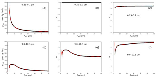
Figure 4.
Parametrizations for volume extinction coefficient divided by the liquid water content (LWC) (a,d), single scattering albedo (b,e), and asymmetry factor (c,f). The upper and lower rows refer to wavelengths of 0.25–0.7 µm (SW) (a–c) and 9.0–10.3 µm (LW)(d–f) intervals respectively. The black line is composed of HS93 original data spectrally averaged for our wavelength intervals and the red dashed line denotes the parametrization fit model. As can be seen from the plots, the fit is invalid for an effective radius smaller than 2.5 µm. These fits showed the correct asymptotic behavior up to 7000 µm (not shown here).
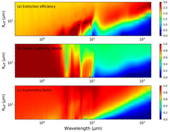
Figure 5.
Contours of the extinction efficiency (a), single-scattering albedo (b), and asymmetry factor (c) of liquid droplets as a function of effective radius and wavelength. The extinction coefficient was calculated using Equation (36) but replacing solid ice density with liquid water density (997 kg·m−3).
3. Model Description
The optical properties parametrizations obtained in Section 2 were implemented in two NWP models COSMO [42,43,44,45,46] and ICON [47,48]. In the next section, the sensitivity tests are performed using the COSMO model. Hence, a more detailed description of this model is provided below. COSMO is based on the primitive thermo-hydrodynamic equations that describe non-hydrostatic compressible flow in a moist atmosphere. The model uses a rotated geographical Arakawa C-grid and generalized terrain-following height coordinates with a Lorenz vertical staggering method. Its vertical extension reaches 23.5 km (about 30 hPa) with 60 model levels in the atmosphere. It uses a two-time-level integration scheme based on the Runge–Kutta method of third order for the prediction of the three Cartesian wind components u, v, and w, the pressure perturbation p′ from a hydrostatic base state and the temperature perturbation T′. A fifth-order upwind scheme is used for their horizontal advection. The default version of the COSMO model uses 1-moment bulk microphysical parameterization. In addition to the mass fraction of water vapor, the microphysical prognostic variables are liquid water contents of cloud water and rain, and ice water contents of cloud ice, snow, and graupel. As shown in Section 2, the parametrizations of the optical properties require the knowledge of the effective radius of cloud water and rain , and of the generalized effective size of cloud ice, snow, and graupel . in (2.28) and [17,49] can be approximated using the ratio of water content to the number concentration using the form where depends on the constant mass-size-relation parameters and the size distribution parameters. Some parametrizations of considers both temperature and IWC for . However, the number concentration of the hydrometeors is not predicted by the model and needs to be diagnosed. In our new implementation, the number concentration of liquid hydrometeors was a tuning parameter, while the number concentration of solid hydrometeors was parametrized as a function of temperature (following Cooper, 1986 [50] for cloud ice and Field et al., 2005 [51] for snow). The default COSMO model RG92 optical properties parametrizations are based on Mie calculations by Stephens (1989) [52] and the parametrizations proposed by Slingo and Schrecker (1982) [30] for water clouds. For ice hydrometeors, only a parametrization based on IWC only is implemented (COSMO internal documentation). In the following section, we analyze the effect of the new optical properties parametrizations on the radiation transfer and demonstrate the important role of particle sizes and .
4. Sensitivity Analysis
In this section, we examine the impact of the new optical properties parametrizations on the radiation transfer and compare it with the default COSMO RG92 scheme under different cloudiness situations. For this purpose, we have utilized the idealized version of the COSMO model [53] to simulate radiation transfer through two types of clouds: warm stratus and cirrus. The characteristics of the simulated clouds are summarized in Table 1.

Table 1.
Simulated clouds in an idealized COSMO version. Seven simulations of warm stratus of different widths and 3 simulations of cirrus of different widths were performed. For each experiment, the cloud heights and temperatures of cloud base and cloud top are mentioned, respectively.
In order to analyze the effect of clouds’ width and microphysical properties on the radiation transfer, seven simulations of warm stratus and three simulations of cirrus were performed. These simulations were intended to test the radiation transfer parametrizations only, and not to mimic real weather events or observation campaigns. However, the variety of simulated conditions (Table 1), together with various pollution conditions (described below), properly represented the expected effect of the new parametrization in real weather events. The implementation of new parametrizations generally influenced the shortwave downwelling solar radiation (or global radiation hereafter) both directly and indirectly. The change in radiative heating lead to a different evolution of the simulated cloud, which in turn influenced the radiation transfer. For simplification, we ignored this feedback mechanism and removed the radiative heating term in the equation for temperature tendency. All the idealized COSMO simulations were performed for 6 hours while the solar zenith angle was fixed to 30°. The domain was chosen to be 100 × 100 km2 with a flat and uniform lower boundary surface and periodic boundary conditions and a horizontal resolution of 0.025° (~2.5 km). Both deep and shallow convection Tiedtke-type schemes were switched off. Each simulation was initiated with vertical profiles of temperature and humidity suitable for stratiform cloud formation at the chosen heights (Table 1). During the run period, the simulated clouds slightly changed due to evaporation, particle sedimentation, and other processes. However, they continuously covered the entire simulation domain homogeneously. For each simulation, the output fields (global radiation, total water path, etc.) at 5 min steps were averaged over the domain. Ignoring the first 50 min stabilization period, we obtained 51 values for each field for each simulation. Figure 6a compares the global radiation of RG92 and new parametrization for the seven experiments of warm stratus (see Table 1). The global radiation is shown versus the liquid water path (which is combined from seven experiments, 51 points each). Obviously, the global radiation was smaller for thicker clouds. One could see that in the new version, the clouds were optically thinner than in RG92. The global radiation difference was larger for thicker clouds, reaching 20%.

Figure 6.
(a) Global radiation versus liquid water path for 7 experiments of warm stratus assuming droplet number concentration of 500 cm−3. The clear sky reference is marked by a black dot. The default COSMO radiation scheme RG92 (blue dots) and the new scheme (red dots) are presented. (b) Global radiation (red dots) in the new scheme versus cloud-averaged droplets effective radius for experiment 5 of warm stratus (see Table 1) marked by the dashed circle. The red dots from left to right correspond to cloud droplets number concentrations of 1000, 500, 200, 100, 50, 10 . The range of variation in global radiation due to change in effective radius is marked by dashed lines.
As explained in Section 3, the new scheme parametrized the effect of cloud water number concentration on the effective radius, which influenced the optical properties and the global radiation. Thus, for the warm stratus of experiment 5 (see Table 1), six more runs were performed with various number concentrations. Figure 6b shows the effect of cloud water number concentration on global radiation in the new scheme. In contrast to RG92 where the effective radius was not dependent on number concentration, the new scheme showed a significant effect of number concentration and effective radius on the global radiation. Having the same liquid water path, a pristine cloud (number concentration of 10 cm−3) may double the global radiation compared to a polluted one (number concentration of 1000 cm−3). The immense effect on the cloud optical depth due to cloud number concentration variations was thoroughly discussed by Lu and Seinfeld (2005) [54].
Similar to the warm stratus presented in Figure 6a, Figure 7a shows the global radiation versus ice water path for the three experiments of cirrus (see Table 1). In addition to the default RG92 (blue dots), four more versions of the new parametrization are presented (see Section 2.1 for details): the first assumes rough ice particles surfaces (red dots), the second is similar to the first but adding snow particles into consideration (lime green), the third is similar to the second but assuming smooth surfaces (magenta), and the last is similar to the previous but using the forward scattered fraction approximation of instead of the Fu (2007) [18] formulas 37 and 38 (cyan). Obviously, the global radiation was smaller for thicker clouds. In contrast to the warm stratus, the cirrus cloud in the new versions was optically thicker than in RG92. The largest difference from RG92 occurred when assuming rough ice particles and considering snow effects on radiation, where the effect on the global radiation reached 15% (for thick cirrus—experiment 3). Note that considering snow significantly reduced the global radiation (from red to lime green). Note also that the assumption of smooth surfaces made the clouds optically thinner (from lime green to magenta and cyan), and that there was no significant effect of the different assumptions for the forward scattered fraction (cyan and magenta).
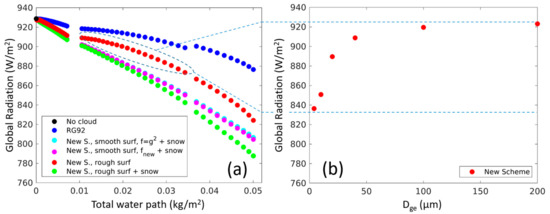
Figure 7.
(a) Global radiation versus ice water path for 3 experiments of cirrus. The clear sky reference is marked by a black dot. In blue dots the default COSMO radiation scheme RG92, red dots represent simulation which assumes rough ice particles surfaces and ignoring snow particles, lime green dots is the result when snow particles are considered, the same but assuming smooth surfaces are in magenta and the last, in cyan, is similar to the previous but using the forward scattered fraction approximation of instead of the Fu (2007) [18] formulas. (b) Global radiation in the third version of the new scheme (red dots) versus cloud-averaged ice particles effective diameter for experiment 2 of cirrus (see Table 1) marked by the dashed circle. The range of variation in global radiation due to change in ice particles effective diameter is marked by dashed lines.
As explained in Section 3, the new scheme parametrized the influence of ice effective diameter on the optical properties and the global radiation. As mentioned, itself was calculated in the model from the ice water content and the number concentration that was a function of temperature. In order to highlight the sensitivity of global radiation to , we implemented an option to artificially determine the constant value at all cloudy grid points. Thus, for the cirrus of experiment 2 (see Table 1), six more runs were performed with various values between 5 and 200 microns. The new version with the assumption of rough needles ignoring the snow effect (red dots in Figure 7a) was chosen for these runs. Figure 7b shows the influence of on the global radiation in the new scheme. In contrast to RG92 where was not introduced, the new scheme showed a significant effect of on global radiation. Having the same ice water path, a cirrus cloud with large particles (an effective diameter of 200 microns) could yield 10% higher global radiation than an identical cloud with small particles (effective diameter of 5 microns).
The important quantity for climate applications is the net heating/cooling effect of the clouds. Usually, during the daytime, the SW incoming radiation heats the atmosphere, which is then cooled down via LW outgoing radiation during night time. We cannot discuss this quantity here since our 6-hour long simulations assumed a fixed solar zenith angle of 30°. However, we can check the effect of the new scheme on the net radiation at the top-of-atmosphere (incoming minus outgoing). Figure 8 presents the net top-of-atmosphere radiation difference between the new scheme and RG92 versus liquid water path for seven experiments of warm stratus (Figure 8a) versus liquid water path for three experiments of cirrus (Figure 8b). Positive (negative) values indicated the warming (cooling) effect by the new scheme with respect to RG92. In Figure 8b, the differences (with respect to RG92) were calculated for the same four versions of the new scheme as described in Figure 7. One could see that the new scheme had a warming effect with respect to RG92 for warm stratus, and a cooling effect for cirrus. Generally, these effects were enhanced (in absolute values) for optically thicker clouds. Note that the assumptions regarding the roughness of the ice particle surfaces were of similar importance to the snow for the net radiation (compare cyan, magenta, and green dots in Figure 8b). It was nicely seen that the consideration of snow enhanced the net cooling, which could be explained by an increase in the cloud albedo.
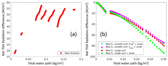
Figure 8.
(a) Net (incoming minus outgoing) top-of-atmosphere (TOA) radiation difference between the new scheme and RG92, versus liquid water path for 7 experiments of warm stratus. Positive values indicate the warming effect of the new scheme with respect to RG92. (b) Net top-of-atmosphere radiation difference between the 4 versions of the new scheme and RG92, versus liquid water path for 3 experiments of cirrus (color details are in the capture of Figure 7a). Negative values indicate the cooling effect of the new scheme with respect to RG92.
5. Real Cases Evaluation
In this section, we compare the default and the new schemes using numerical weather prediction (NWP) simulations with fully interactive radiation. We utilized the convection-permitting configuration of the COSMO model over the eastern Mediterranean (domain 25–39 E/26–36 N) with 2.5 km horizontal resolution and 60 vertical levels reaching 23.5 km. The simulations were initialized and driven by the Integrated Forecast System (IFS) of the European Centre for Medium-Range Weather Forecasts (ECMWF). For each of the COSMO versions, we performed 5 months (July–November 2019) of 78 hours simulations twice a day. Hourly forecasted global radiation was verified against 17 automatic radiation stations over Israel in cloudy conditions. Only cloudy events with observed and simulated cloud cover above 95% were selected for global radiation verification. For observations, the cloudiness products from CMSAF (https://www.cmsaf.eu) were used. The verification was performed for low and high cloudiness situations, separately, as defined by the CMSAF cloud type algorithm. We have assumed that during the verification period high clouds are composed mainly of solid particles and low clouds from liquid droplets. As proof, we have used the simulations to retrieve the temperatures at the cloudy layers which correspond to the observed clouds. Indeed, the temperatures in high cloudiness situations were below −19 °C, while the temperatures in low cloudiness situations were above 6 °C. Figure 9 shows the results of the separate verification for low cloudiness (Figure 9a,b) and high cloudiness (Figure 9c,d). Figure 9a,c show the distribution of the error (bias) having a bin width of 50 W/m2. A positive error meant model overestimation. Figure 9b,d show the mean diurnal cycle of the global radiation in both observations (black), the default COSMO RG92 version (blue), and the new version (red). In the idealized simulations presented in Section 4, the global radiation by the two COSMO versions was compared in identical cloudiness conditions. In real case simulations with cloudy conditions, having the same 3D cloud cover, water content and particle effective radius in various model versions and reality are hardly achievable. Therefore, the verification conclusions regarding radiation transfer through clouds may be drawn only statistically based on many events, yet assuming that there are no biases in the forecasts of cloudiness depth. In order to reduce the noise originating in comparing the global radiation in cases of significantly different cloud depths, we ignored the events where the global radiation absolute error was above 200 W/m2 due to cloud thickness differences (see Figure 9). Panels a and b show that the new version, having the updated clouds optical properties, reduced the mean bias from −7.1 to + 3 W/m2. In agreement with Figure 6, the new version resulted in slightly higher global radiation. However, the improvement was not statistically significant. The improvement was much more evident for high cloudiness, where the new version reduced the global radiation overestimation from 15.5 to 1.2 W/m2. The reduction in the global radiation by the new version was as expected from idealized COSMO runs (Figure 7) not only due to the change in ice optical properties parametrization but also due to the inclusion of snow in the radiation transfer scheme.
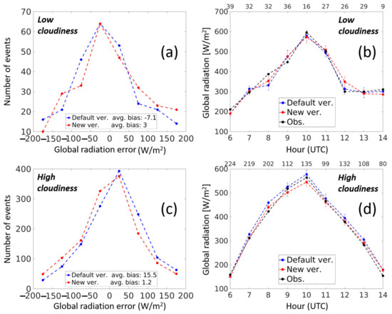
Figure 9.
Hourly global radiation verification for low cloudiness (a,b) and high cloudiness (c,d) during the period July–November 2019. Panels (a,c) show the distribution of the bias (model minus observation). Panels (b,d) show the mean diurnal cycle of the global radiation in both observations (black), the default COSMO RG92 version (blue), and the new version (red). During the verification period, each of the COSMO versions was simulated twice a day with 78 hours lead-time and verified against 17 automatic radiation stations over Israel.
6. Conclusions
In this study, we re-calculate liquid water droplets and ice particles’ optical properties in clouds using former works available in the literature regarding these hydrometeors. For water droplets, a unified and general mathematical formulation was used for both the short wave and long wave regimes. For ice particles, thousands of generalized gamma distributions were assumed to simulate a broad range of ice clouds. An advanced spectral integration method was introduced offering more practical use in NWP and climate models.
Sensitivity analysis using COSMO ideal framework to simulate stratus water clouds showed a small impact of optical properties parametrization on clouds optical thickness and as expected, the 5 months of real COSMO simulations have indicated a relatively small improvement of the new scheme compared to the default parameterization. Nevertheless, a much greater effect on the results was obtained for variation in the effective radius. This emphasizes the advantage of implementing a realistic cloud number concentration calculation. A possible solution could be to use prognostic aerosols in cloud formation schemes. The same argument holds for the ice particles’ effective size and the need for precise simulations of nucleation processes in cirrus clouds. As for ice clouds, we showed a much greater impact of the new ice particles’ optical properties parametrizations on radiation. We also showed that both the inclusion of snow particles and the smooth/rough surface assumptions can have a significant effect on the net surface radiation of a few tens of W/m2. The calculation of the energy balance of the Earth is strongly dependent on ice and water optical properties and the hydrometeor’s effective size. The large (> 50 W/m2) uncertainties can be critical in any climate model but maybe masked out due to the partial cloud cover of the Earth or by cancelation effects such as between liquid and ice particles as demonstrated in our work. A web application for ice and liquid hydrometeors optical properties parametrizations based on this work was created and available for the public on the COSMO webpage (www.cosmo-model.org/content/tasks/operational/ims/cloudOptics/default.htm).
Author Contributions
Conceptualization, U.B., Q.F., and H.B.M.; methodology, U.B., H.B.M.; software, H.B.M., P.K, U.B. and Q.F.; validation, P.K.; formal analysis, H.B.M., U.B. and Q.F.; investigation, H.B.M., U.B., P.K. and Q.F.; data curation, H.B.M.; writing—original draft preparation, H.B.M. and P.K.; writing—review and editing, Q.F. and Y.L.; visualization, H.B.M. and P.K.; supervision, U.B. and Y.L.; project administration, H.B.M. All authors have read and agreed to the published version of the manuscript.
Funding
This research received no external funding.
Data Availability Statement
The data presented in this study are available on request from the corresponding author. The data are not publicly available due to memory size limits. The reader may refer to the online cloud optics web-application mentioned at the end of the manuscript for further details.
Acknowledgments
This study was performed within the Testing and Tuning of the Revised Cloud Radiation Coupling T2(RC)2 priority project in the COSMO consortium. We thank Theodore Andreadis for creating and maintaining the COSMO web application for cloud optics and Robin Hogan for fruitful discussions and data comparisons.
Conflicts of Interest
The authors declare no conflict of interest.
References
- Khain, A.P.; Pinsky, M. Physical Processes in Clouds and Cloud Modeling; Cambridge University Press (CUP): Cambridge, UK, 2018; p. 642. [Google Scholar]
- Twomey, S. The Influence of Pollution on the Shortwave Albedo of Clouds. J. Atmos. Sci. 1997, 34, 1149–1152. [Google Scholar] [CrossRef]
- Rosenfeld, D. Aerosol-Cloud Interactions Control of Earth Radiation and Latent Heat Release Budgets. Space Sci. Rev. 2007, 125, 149–157. [Google Scholar] [CrossRef]
- Soden, B.J.; Held, I.M.; Colman, R.; Shell, K.M.; Kiehl, J.T.; Shields, C.A. Quantifying climate feedbacks using ra-diative kernels. J. Clim. 2008, 21, 3504–3520. [Google Scholar] [CrossRef]
- Stocker, T.F.; Qin, D.; Plattner, G.K.; Tignor, M.M.; Allen, S.K.; Boschung, J.; Nauels, A.; Xia, Y.; Bex, V.; Midgley, P.M. Climate Change 2013: The Physical Science Basis. Contribution of Working Group I to the fifth Assessment Report of IPCC the Intergovernmental Panel on Climate Change. Available online: https://www.ipcc.ch/site/assets/uploads/2017/09/WG1AR5_Frontmatter_FINAL.pdf (accessed on 6 January 2021).
- Yang, P.; Liou, K.N.; Wyser, K.; Mitchell, D. Parameterization of the scattering and absorption properties of in-dividual ice crystals. J. Geophys. Res. 2000, 105, 4699–4718. [Google Scholar] [CrossRef]
- Rossow, W.B.; Schiffer, R.A. Advances in understanding clouds from ISCCP. Bull. Amer. Meteorol. Soc. 1999, 80, 2261–2288. [Google Scholar] [CrossRef]
- Sassen, K.; Wang, Z.; Liu, D. Global Distribution of Cirrus Clouds from CloudSat/Cloud-Aerosol Lidar and Infra-red Pathfinder Satellite Observations (CALIPSO) Measurements. Available online: https://agupubs.onlinelibrary.wiley.com/doi/full/10.1029/2008JD009972 (accessed on 6 January 2021).
- Gasparini, B.; Lohmann, U. Why cirrus cloud seeding cannot substantially cool the planet. J. Geophys. Res. Atmos. 2016, 121, 4877–4893. [Google Scholar] [CrossRef]
- Gruber, S.; Blahak, U.; Haenel, F.; Kottmeier, C.; Leisner, T.; Muskatel, H.; Storelvmo, T.; Vogel, B. A Process Study on Thinning of Arctic Winter Cirrus Clouds With High-Resolution ICON-ART Simulations. J. Geophys. Res. Atmos. 2019, 124, 5860–5888. [Google Scholar] [CrossRef]
- Fu, Q.; Liou, K.N. Parameterization of the Radiative Properties of Cirrus Clouds. J. Atmos. Sci. 1993, 50, 2008–2025. [Google Scholar] [CrossRef]
- Yang, P.; Bi, L.; Baum, B.A.; Liou, K.-N.; Kattawar, G.W.; Mishchenko, M.I.; Cole, B. Spectrally Consistent Scattering, Absorption, and Polarization Properties of Atmospheric Ice Crystals at Wavelengths from 0.2 to 100 μm. J. Atmos. Sci. 2013, 70, 330–347. [Google Scholar] [CrossRef]
- Yang, P.; Ding, J.; Panetta, R.L.; Liou, K.N.; Kattawar, G.W.; Mishchenko, M. On the Convergence of Numer-ical Computations for Both Exact and Approximate Solutions for Electromagnetic Scattering by Nonspherical Dielectric Particles. Electromagn. Waves 2019, 164, 27–61. [Google Scholar] [CrossRef]
- Takano, Y.; Liou, K.-N. Solar Radiative Transfer in Cirrus Clouds. Part I: Single-Scattering and Optical Properties of Hexagonal Ice Crystals. J. Atmos. Sci. 1989, 46, 3–19. [Google Scholar] [CrossRef]
- Fu, Q. An Accurate Parameterization of the Solar Radiative Properties of Cirrus Clouds for Climate Models. J. Clim. 1996, 9, 2058–2082. [Google Scholar] [CrossRef]
- Macke, A.; Mueller, J.; Raschke, E. Single Scattering Properties of Atmospheric Ice Crystals. J. Atmos. Sci. 1996, 53, 2813–2825. [Google Scholar] [CrossRef]
- Fu, Q.; Yang, P.; Sun, W.B. An Accurate Parameterization of the Infrared Radiative Properties of Cirrus Clouds for Climate Models. J. Clim. 1998, 11, 2223–2237. [Google Scholar] [CrossRef]
- Fu, Q. A New Parameterization of an Asymmetry Factor of Cirrus Clouds for Climate Models. J. Atmos. Sci. 2007, 64, 4140–4150. [Google Scholar] [CrossRef]
- Yang, P.; Liou, K.N. Light scattering by hexagonal ice crystals: Comparison of finite-difference time domain and geometric optics models. J. Opt. Soc. Am. A 1995, 12, 162–176. [Google Scholar] [CrossRef]
- Thorsen, T.J.; Fu, Q. Automated Retrieval of Cloud and Aerosol Properties from the ARM Raman Lidar. Part II Extinction. J. Atmos. Ocean. Technol. 2015, 32, 1999–2023. [Google Scholar] [CrossRef]
- Fu, Q.; Liou, K.N.; Cribb, M.C.; Charlock, T.P.; Grossman, A. Multiple Scattering Parameterization in Thermal Infrared Radiative Transfer. J. Atmos. Sci. 1997, 54, 2799–2812. [Google Scholar] [CrossRef]
- Yang, P.; Liou, K.N. Finite-difference time domain method for light scattering by small ice crystals in three-dimensional space. J. Opt. Soc. Am. A 1996, 13, 2072–2085. [Google Scholar] [CrossRef]
- Baum, B.A.; Heymsfield, A.J.; Yang, P.; Bedka, S.T. Bulk Scattering Properties for the Remote Sensing of Ice Clouds. Part I: Microphysical Data and Models. J. Appl. Meteorol. 2005, 44, 1885–1895. [Google Scholar] [CrossRef]
- Baum, B.A.; Yang, P.; Heymsfield, A.J.; Schmitt, C.G.; Xie, Y.; Bansemer, A.; Hu, Y.; Zhang, Z.-B. Improvements in Shortwave Bulk Scattering and Absorption Models for the Remote Sensing of Ice Clouds. J. Appl. Meteorol. Clim. 2011, 50, 1037–1056. [Google Scholar] [CrossRef]
- Baum, B.A.; Yang, P.; Heymsfield, A.J.; Bansemer, A.; Cole, B.H.; Merrelli, A.; Schmitt, C.; Wang, C. Ice cloud single-scattering property models with the full phase matrix at wavelengths from 0.2 to 100 µm. J. Quant. Spectrosc. Radiat. Transf. 2014, 146, 123–139. [Google Scholar] [CrossRef]
- Hansen, J.E.; Travis, L.D. Light scattering in planetary atmospheres. Space Sci. Rev. 1974, 16, 527–610. [Google Scholar] [CrossRef]
- Khain, P.; Heiblum, R.; Blahak, U.; Levi, Y.; Muskatel, H.; Vadislavsky, E.; Altaratz, O.; Koren, I.; Dagan, G.; Shpund, J.; et al. Parameterization of Vertical Profiles of Governing Microphysical Parameters of Shallow Cumulus Cloud Ensembles Using LES with Bin Microphysics. J. Atmos. Sci. 2019, 76, 533–560. [Google Scholar] [CrossRef]
- Hu, Y.X.; Stamnes, K. An Accurate Parameterization of the Radiative Properties of Water Clouds Suitable for Use in Climate Models. J. Clim. 1993, 6, 728–742. [Google Scholar] [CrossRef]
- Wiscombe, W.J. The Delta-Eddington Approximation for a Vertically Inhomogeneous Atmosphere; NCAR Technical Note NCAR/TN-121+STR; NCAR: Boulder, CO, USA, 1977. [Google Scholar]
- Slingo, A.; Schrecker, H.M. On the shortwave radiative properties of stratiform water clouds. Q. J. R. Meteorol. Soc. 1982, 108, 407–426. [Google Scholar] [CrossRef]
- Slingo, A. A GCM Parameterization for the Shortwave Radiative Properties of Water Clouds. J. Atmos. Sci. 1989, 46, 1419–1427. [Google Scholar] [CrossRef]
- Edwards, J.M.; Slingo, A. Studies with a flexible new radiation code. I: Choosing a configuration for a large-scale model. Q. J. R. Meteorol. Soc. 1996, 122, 689–719. [Google Scholar] [CrossRef]
- Stephens, G.L. The Parameterization of Radiation for Numerical Weather Prediction and Climate Models. Mon. Weather. Rev. 1984, 112, 826–867. [Google Scholar] [CrossRef]
- Lindner, T.H.; Li, J. Parameterization of the Optical Properties for Water Clouds in the Infrared. J. Clim. 2000, 13, 1797–1805. [Google Scholar] [CrossRef]
- Baran, A.J.; Hill, P.; Furtado, K.; Field, P.; Manners, J. A Coupled Cloud Physics–Radiation Parameterization of the Bulk Optical Properties of Cirrus and Its Impact on the Met Office Unified Model Global Atmosphere 5.0 Configuration. J. Clim. 2014, 27, 7725–7752. [Google Scholar] [CrossRef]
- Baran, A.J.; Hill, P.; Walters, D.; Hardiman, S.C.; Furtado, K.; Field, P.R.; Manners, J. The Impact of Two Coupled Cirrus Microphysics–Radiation Parameterizations on the Temperature and Specific Humidity Biases in the Tropical Tropopause Layer in a Climate Model. J. Clim. 2016, 29, 5299–5316. [Google Scholar] [CrossRef]
- Petty, G.W.; Huang, W. The Modified Gamma Size Distribution Applied to Inhomogeneous and Non-spherical Particles: Key Relationships and Conversions. J. Atmos. Sci. 2011, 68, 1460–1473. [Google Scholar] [CrossRef]
- Smith, H.R.; Baran, A.J.; Hesse, E.; Hill, P.G.; Connolly, P.J.; Webb, A. Using laboratory and field measurements to constrain a single habit shortwave optical parameterization for cirrus. Atmos. Res. 2016, 180, 226–240. [Google Scholar] [CrossRef]
- Hogan, R.J.; Bozzo, A. A Flexible and Efficient Radiation Scheme for the ECMWF Model. J. Adv. Model. Earth Syst. 2018, 10, 1990–2008. [Google Scholar] [CrossRef]
- Ritter, B.; Geleyn, J. A Comprehensive Radiation Scheme for Numerical Weather Prediction Models with Potential Applications in Climate Simulations. Mon. Weather Rev. 1992, 120, 303–325. [Google Scholar] [CrossRef]
- Joseph, J.H.; Wiscombe, W.J.; Weinman, J.A. The Delta-Eddington Approximation for Radiative Flux Transfer. J. Atmos. Sci. 1976, 33, 2452–2459. [Google Scholar] [CrossRef]
- Steppeler, J.; Doms, G.; Schattler, U.; Bitzer, H.W.; Gassmann, A.; Damrath, U.; Gregoric, G. Meso gamma scale forecasts by nonhydrostatic model LM. Meteorol. Atmos. Phys. 2003, 82, 75–96. [Google Scholar] [CrossRef]
- Baldauf, M.; Seifert, A.; Förstner, J.; Majewski, D.; Raschendorfer, M.; Reinhardt, T. Operational convective-scale numer-ical weather prediction with the COSMO model: Description and sensitivities. Mon. Weather Rev. 2011, 139, 3887–3905. [Google Scholar] [CrossRef]
- Doms, G.; Foerstner, J.; Heise, E.; Herzog, H.J.; Mironov, D.; Raschendorfer, M.; Reinhardt, T.; Ritter, B.; Schrodin, R.; Schulz, J.P.; et al. A Description of the Nonhydrostatic Regional COSMO Model, part 2: Physical Parameterization. Available online: http://www.cosmo-model.org (accessed on 6 January 2021).
- Kunz, M.; Blahak, U.; Handwerker, J.; Schmidberger, M.; Punge, H.J.; Mohr, S.; Fluck, E.; Bedka, K.M. The severe hailstorm in southwest Germany on 28 July 2013: Characteristics, impacts and meteorological conditions. Q. J. R. Meteorol. Soc. 2018, 144, 231–250. [Google Scholar] [CrossRef]
- Khain, P.; Levi, Y.; Muskatel, H.; Shtivelman, A.; Vadislavsky, E.; Stav, N. Effect of shallow convection parametrization on cloud resolving NWP forecasts over the Eastern Mediterranean. Atmos. Res. 2021, 247, 105213. [Google Scholar] [CrossRef]
- Zängl, G.; Reinert, D.; Ripodas, P.; Baldauf, M. The ICON (ICOsahedral Non-hydrostatic) modelling frame-work of DWD and MPI-M: Description of the non-hydrostatic dynamical core. Q. J. R. Meteorol. Soc. 2015, 141, 563–579. [Google Scholar] [CrossRef]
- Giorgetta, M.A.; Brokopf, R.; Crueger, T.; Esch, M.; Fiedler, S.; Helmert, J.; Hohenegger, C.; Kornblueh, L.; Köhler, M.; Manzini, E.; et al. ICON-A, the Atmosphere Component of the ICON Earth System Model: I. Model Description. J. Adv. Model. Earth Syst. 2018, 10, 1613–1637. [Google Scholar] [CrossRef]
- Key, J.R.; Yang, P.; Baum, B.A.; Nasiri, S.L. Parameterization of shortwave ice cloud optical properties for various particle habits. J. Geophys. Res. Space Phys. 2002, 107. [Google Scholar] [CrossRef]
- Braham, R.R.; Cooper, W.A.; Cotton, W.R.; Elliot, R.D.; Flueck, J.A.; Fritsch, J.M.; Gagin, A.; Grant, L.O.; Heymsfield, A.J.; Hill, G.E.; et al. Precipitation Enhancement—A Scientific Challenge. Precip. Enhanc. Sci. Chall. 1986, 29–32. [Google Scholar] [CrossRef]
- Field, P.R.; Hogan, R.J.; Brown, P.R.A.; Illingworth, A.J.; Choularton, T.; Cotton, R.J. Parametrization of ice-particle size distributions for mid-latitude stratiform cloud. Q. J. R. Meteorol. Soc. 2005, 131, 1997–2017. [Google Scholar] [CrossRef]
- Stephens, G.L. Optical properties of eight water cloud types. In CSIRO: Division of Atmospheric Physics; Tech. Report 36; CSIRO: Canberra, Australia, 1979. [Google Scholar]
- Blahak, U. Simulating Idealized Cases with theCOSMO-Model. Manual, Consortium for Small Scale Modelling. Available online: http://www.cosmo-model.org/content/model/documentation/core/artifdocu.pdf (accessed on 6 January 2021).
- Lu, M.-L.; Seinfeld, J.H. Study of the Aerosol Indirect Effect by Large-Eddy Simulation of Marine Stratocumulus. J. Atmos. Sci. 2005, 62, 3909–3932. [Google Scholar] [CrossRef]
Publisher’s Note: MDPI stays neutral with regard to jurisdictional claims in published maps and institutional affiliations. |
© 2021 by the authors. Licensee MDPI, Basel, Switzerland. This article is an open access article distributed under the terms and conditions of the Creative Commons Attribution (CC BY) license (http://creativecommons.org/licenses/by/4.0/).