Article

A Novel Hybrid Machine Learning Method (OR-ELM-AR) Used in Forecast of PM2.5 Concentrations and Its Forecast Performance Evaluation

1
School of Economics, Shanghai University, Shanghai 200444, China
2
School of Environmental and Chemical Engineering, Shanghai University, Shanghai 200444, China
3
Key Laboratory of Organic Compound Pollution Control Engineering, Shanghai University, Shanghai 200444, China
4
The Joint Graduate School of Energy and Environment, King Mongkut’s University of Technology Thonburi, Bangkok 10140, Thailand
5
Center of Excellence on Energy Technology and Environment, Ministry of Higher Education, Science, Research and Innovation, Bangkok 10140, Thailand
*
Authors to whom correspondence should be addressed.
Atmosphere 2021, 12(1), 78; https://doi.org/10.3390/atmos12010078
Submission received: 27 November 2020 / Revised: 31 December 2020 / Accepted: 2 January 2021 / Published: 6 January 2021
(This article belongs to the Special Issue Air Quality Management)

Abstract

:
Accurate forecast of PM2.5 pollution is highly needed for the timely prevention of haze pollution in many cities suffered from frequent haze pollution. In this work, an online recurrent extreme learning machine (OR-ELM) technique with online data update was used in the forecast of PM2.5 pollution for the first time, and a hybrid model (OR-ELM-AR) by combining autoregressive (AR) model was proposed to enhance its forecast ability to capture the variations of hourly PM2.5 concentration. Evaluation of forecast performances in terms of pollution levels, forecast times, spatial distributions were conducted over the Yangtze River Delta (YRD) region, China. Results indicated that the OR-ELM-AR model could quickly respond to short-term changes and had better forecast performance. Therefore, the OR-ELM-AR model is a promising tool for air pollution forecast of supporting the government to take urgent actions to reduce the frequency and severity of haze pollution in cities or regions.

Graphical Abstract

1. Introduction

With rapid urbanization and economic development, China has confronted severe haze pollution, with surface concentrations of fine particulate matter (PM2.5) exceeding air quality standards in recent decades [1,2,3,4]. A high concentration of PM2.5 not only affects people’s daily life and health but also exhibits negative impacts on the social economy and climate change [5,6,7]. Therefore, it is essential to predict PM2.5 concentration accurately in advance so that the government could make decisions and take effective emergency control measures timely to reduce pollution levels in advance and thus to protect public health. However, the accurate forecast of hourly PM2.5 concentration is still a great challenge due to the complexity of its formation mechanisms of PM2.5 [4,8,9,10]. Variations of PM2.5 concentration usually depends on changes in emission and meteorological condition [2,10]. Furthermore, PM2.5 was highly nonlinear related to them, as many studies reported [7,11].
In recent years, researchers have made substantial contributions to the prediction of PM2.5 concentrations by machine-learning methods [8,12,13]. The forecasting models based on machine learning techniques are generally divided into two categories, namely offline models and online models [14]. Offline models can be further divided into two subcategories, including the single models and hybrid models. Single models mainly include linear regression models, gray models, Bayesian, support vector machines, neural networks, as well as other algorithms-led artificial intelligence methods. In many studies [7], linear models, such as the autoregressive integrated moving average model (ARIMA) and mixed logistic regression (MLR), were used to predict the concentration of PM2.5 and PM10. If the PM2.5 concentration sequence is linear, the forecast results of ARIMA and MLR will be more reliable and interpretative [15]. However, temporal variations of particulate matters are highly nonlinear, non-stationary and irregular sequences in real situations. The limitation of linear models is that their predictions rely too much on the linear mapping capability. Compared with linear models, nonlinear models are better at predicting extreme concentrations [6]. As a typical kind of nonlinear model, artificial intelligence algorithms, such as an artificial neural network (ANN), are widely used to predict particle concentration [8,13,16,17]. However, nonlinear models have their own limitations. For example, they are easy to cause local optimization and overfitting problems [18]. In order to improve the forecast performance of the model, increasing researchers have tried to use hybrid models in recent years [6,19,20]. Most hybrid models are composed of linear models and nonlinear models [19,21]. With the development of hybrid models, the idea of “decomposition and aggregation” is gradually applied to the prediction in time-series cases [22] as a supplement to the deterministic models and statistical models. Studies have shown that the “decomposition-collection” method, as part of the hybrid models, can greatly improve the accuracy of PM2.5 prediction [13,20].
However, time-series data of PM2.5 concentration arrives in the form of data streams, and the distribution of data changes over time [23,24]. Online learning models with incremental update capability should be more suitable for predicting PM2.5 concentration because of the nonlinear and non-stationary time-series of PM2.5 data. The online sequential extreme learning machine (OS-ELM) is an emerging online learning algorithm proposed by [25]. This model was used to predict a particular matter in the atmosphere and achieved a better forecast performance than the ELM algorithm [26]. However, OS-ELM has two obvious shortcomings. One is that the input weight cannot be adjusted; the other is that the cyclic neural network cannot be trained. Park and Kim (2017) overcame the shortcomings of OS-ELM by adding the auto-encoding with normalization and feedback input for the recurrent neural network (RNN) structure, and an online recurrent extreme learning machine (OR-ELM) was proposed to forecast New-York city taxi passenger count [14]. Their results showed that OR-ELM could rapidly adapt to the pattern change, and the forecast error was minimized compared with OS-ELM and other online-sequential learning algorithms [14]. The OR-ELM model has shown to be a promising tool to capture nonlinear and non-stationary time-series features with rapid update capability. However, the OR-ELM model has not been used in hourly PM2.5 prediction so far.
In this work, the OR-ELM model was applied to forecast PM2.5 concentrations for the first time. In addition, the hybrid model of OR-ELM-AR was proposed by coupling with the autoregressive (AR) model based on the OR-ELM model in order to deeply explore information from its residuals. The performance evaluations were conducted by comparison with observed data based on different time periods and pollution levels. There were seven criteria, including mean error (bias), mean absolute error (MAE), root-mean-squared error (RMSE), index of agreement (IOA), fractional bias (FBIAS), fractional error (FERROR) and correlation (R), which were used to evaluate the forecast performance. Spatial forecast performance was also examined through 41 prefecture-level cities over the Yangtze River Delta (YRD) region, which is one of the heavy PM2.5 polluted regions in China in recent decades. To better understand the forecast performance of OR-ELM-AR, LSTM, OS-ELM and OR-ELM models were employed to compare with the forecast performance of OR-ELM-AR.

2. Methods and Data Source

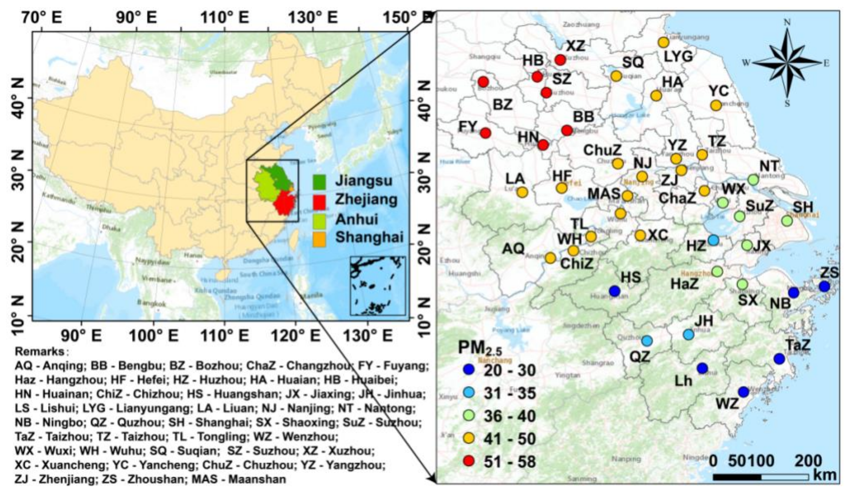
2.1. Study Domain and Data Source

As one of the most densely populated regions, the YRD region, located in eastern China, has a population of over 150 million, accounting for 11% of the total population in China. It is also one of the most economically developed regions in China. The YRD region consists of Shanghai Municipality and three provinces, covering 41 prefecture-level cities, as shown in Figure 1. Nanjing, Hangzhou and Hefei are the capital cities of Jiangsu, Zhejiang and Anhui Provinces, respectively. Data of observed hourly PM2.5 concentrations can be obtained from the China Urban Air Quality Real-Time Publishing Platform (http://106.37.208.233:20035/), which was supported by the Ministry of Ecology and Environment of the People’s Republic of China (MEEP). The instrument operation and management, data quality assurance and quality control of these data are all performed in strict compliance with NAAQS guidelines (GB 3095-2012).
The training data we used in this study are the data of hourly PM2.5 concentrations, which were continuously observed in every city from 2017/1/1 00:00 to 2019/12/31 23:00. For each city, after training using past 200 samples of PM2.5 concentration, the models were established to predict the PM2.5 concentrations at the next 1st to 6th hour. There are 26,280 samples, which involve data of hourly PM2.5 concentrations at one city during this time period, which were used to be the training data for the forecast in the same city. Missing data accounts for 0.6% of the whole series. The period of consecutive missing data in Huangshan city was 12 h. Because of the best air quality with low concentrations of PM2.5 in Huangshan city compared with other cities in the YRD region, the effect of missing data is negligible. Missing data were filled with data of previous hours in the time-series.

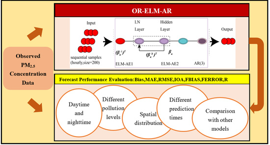
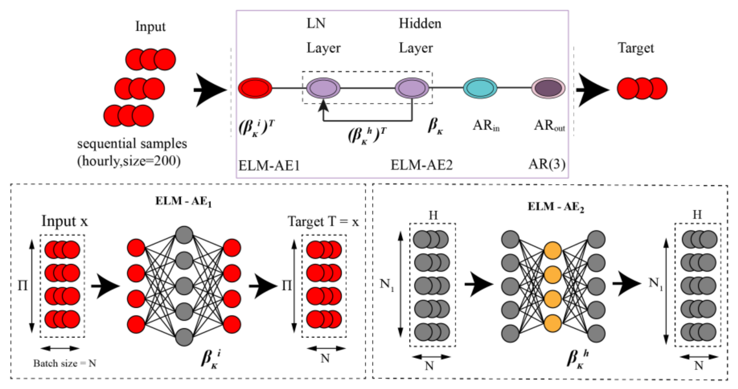
2.2. Model Framework of OR-ELM-AR and Forecasting Process

Based on the OR-ELM model [14], a hybrid model combining an online sequential extreme learning machine with the AR model (OR-ELM-AR) was developed in this study, as illustrated by Figure 2. It consists of three neural networks and a link with the AR model. The core of OR-ELM-AR is a recurrent neural network (RNN) for the prediction, extended by an AR model to deeply explore information from its residuals. Two single-hidden layer feed-forward neural networks (ELM-auto-encoder, ELM-AE), referred to as ELM-AE1 and ELM-AE2, were designed to learn RNN′s input weights and hidden weights, respectively. All the observed data were separated into two parts, namely the training dataset and the test dataset. Samples in the training dataset were input to the model as a batch of size 200 sequentially, with one complex function generated from the training process. This function was used to forecast the PM2.5 concentration during the time period of the test dataset. The forecast performance can be evaluated by comparison of the forecast concentrations and the observed concentrations in the test dataset with the help of several metrics.
The training process of the OR-ELM-AR model consists of three stages, as follows:
Stage 1: initialization phase:
The initial input weights and hidden weights were randomly assigned with a mean-zero and a standard deviation of one. The initial output weights were set by fully online initialization method: β 0 = 0 ,   P 0 = I C 1 , where I is a unit diagonal matrix, and C is a constant.
Stage 2: an online learning phase
The main algorithm was to learn sequential data by recursive least-squares method (RLS). The output weight is as follows:
β t + 1 = RLS ( A , Z , λ )
the definition of RLS is as follows:
W t + 1 = f n o r m A
β t + 1 = β t + P t + 1 W t + 1 T Z W t + 1 β t
P t + 1 = 1 λ P t P t W t + 1 T ( λ 2 + λ W t + 1 P t W t + 1 T ) 1 W t + 1 P t
where A is an input weight matrix, and W is an output weight matrix. N o r m   · is the normalization method, which is called layer normalization (LN) and is applied to avoid degradation problems. The regret factor λ enables the algorithm to continually forget the outdated data and adapt to new patterns. If λ   =   1 , there is no regret.
Once the training samples were updated, the input weights were updated correspondingly and the hidden weight successively by RLS in which the regret factor is included and the hidden weight A t is used, as follows:
Update   the   input   weight :   A i   =   A t + 1 i T X t + 1
β t + 1 i   =   RLS ( A i , X t + 1 , λ )
Update   the   hidden   weight :   A h = A t + 1 h T W t
β t + 1 h = RLS ( A h ,   W t , λ )
Update   the   output   weight :   A = A t + 1 X t + 1 + β t + 1 h T W t
β t + 1 = RLS ( A ,   Y t + 1 , 1 )
Stage 3: autoregression phase
According to Equation (11), residuals y t are extracted from the forecast results of OR-ELM, and autoregression was conducted to generate new residuals y t + 1 , as shown in Equation (12). Finally, the ultimate prediction of PM2.5 concentration are p r e d i c t e d t + 1 + y t + 1   .
y t = t a r g e t t p r e d i c t e d t
y t + 1 = φ 1 y t + φ 2 y t 1 + φ 3 y t 2 + ε t + 1

2.3. Evaluation Methods

The forecast results of OR-ELM-AR were evaluated by comparing with the observed data based on several statistical metrics, including mean error (bias), mean absolute error (MAE), root-mean-squared error (RMSE), index of agreement (IOA), fractional bias (FBIAS), fractional error (FERROR) and correlation coefficient (R). Definitions of these metrics are shown in Table 1. In order to evaluate the robustness of forecast performances, these metrics were calculated for different cases: (1) at different forecasting time from the first hour to the sixth hour; (2) at different PM2.5 pollution levels; (3) during time periods of daytime and nighttime, respectively; (4) spatial distribution of forecast over the whole YRD region. In addition, LSTM, OS-ELM and OR-ELM were also used, and their performances were compared with OR-ELM-AR for better understanding the advantage of the OR-ELM-AR model in forecast ability [27].

3. Results

3.1. General Temporal-Spatial Patterns of PM2.5 Pollution

The annual PM2.5 concentration for attainment should be lower than 35 μg/m3, according to the national ambient air quality standards (NAAQS). The PM2.5 concentration of cities in the central and northern YRD region in 2018 fail to meet the standards, as shown in Figure 1 (right), and the concentrations in the north YRD region are still high. In order to explore the mid-to-long-term trend of PM2.5 pollution variations, we used a moving average of 20 weeks (nearly 5 months), which is often used by researchers to describe the middle-long term trend [28]. Figure S1 shows 20 weeks moving average of PM2.5 concentration in three different typical cities (Nanjing, Shanghai, and Xuzhou): the moving average in Shanghai was lower than 60 μg/m3 whereas that in Xuzhou was much higher than 60 μg/m3 for most values. Nevertheless, these three cities all present the same seasonal pattern that the moving average PM2.5 concentration increased from November to April mainly due to high concentrations in winter and decreased from April to October mainly due to relatively low concentrations in summer. January, April, July and October are the representative months of winter, spring, summer and autumn, respectively, in the YRD region.
From the perspective of the spatial distribution, the heavily polluted areas were mainly in the northern part of the YRD region, of which the pollution in northern Anhui and Xuzhou in Jiangsu Province was particularly heavy (Figure 1). PM2.5 concentration in several cities in southern Zhejiang has met the NAAQS standard. Pollution in the central and eastern YRD region and coastal cities in Jiangsu was at a moderate level.
The diurnal variations of the average PM2.5 concentration for 41 cities in the YRD region are shown in Figure S2. The concentration in summer is the lowest, and the concentration in winter is the highest. The concentration in April 2019 was significantly lower than that in the previous year. Differences between seasons and between years are not only related to emission changes but also to variations in the meteorological conditions. In general, there was a peak of PM2.5 during 08:00–10:00 a.m., followed by a decrease and then an increase again at night.
As shown in Figure S2, the average PM2.5 concentration in January 2018 in Shanghai, Nanjing and Xuzhou were all higher than those in the same period in 2017. The high peaks all occurred at 11:00 a.m., and both Shanghai and Nanjing showed second peaks between 20:00–21:00 at night. According to the observed hourly concentration in these three cities, the relatively high PM2.5 concentrations and diurnal variations in these three cities were mainly dominated by several pollution episodes with heavy pollution during the daytime in January 2018. There were more heavy-pollution episodes in January 2018 than in the same period in 2017, which also can partially be explained that the overall PM2.5 concentration in January 2018 in the YRD region was significantly higher than that in the same period in 2017. Based on the average diurnal change of PM2.5 concentration over the whole YRD region and in these three cities, the change of concentrations at night was relatively gentle, but the change during the daytime could be dramatic. The differences of daytime (7:00–20:00) and nighttime (21:00–6:00) forecast abilities of OR-ELM-AR model in PM2.5 concentration were examined in this study.

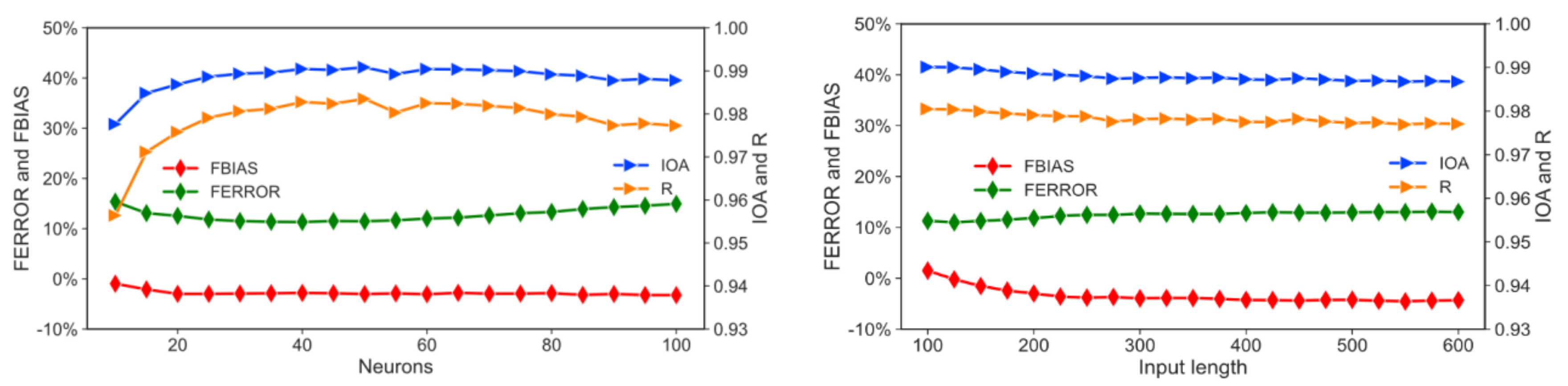
3.2. Optimization of Model Parameters

A total of 26,280 hourly samples were rearranged and fed into the training dataset sequentially by online manner for each city’s forecast. Each training dataset has two parts. One part was a bundle of 200 samples that are set as input data to the model, and the other part was the corresponding observed data in the next few hours are the target data of forecast. These target data are used to evaluate the forecast performance based on several metrics. In a period of training, one train dataset is input to update three weights in the model, and we use the next bundle of data to predict PM2.5 concentration for the next few hours.
To ensure the robustness of the experiments of the OR-ELM-AR model, the impacts of the number of neurons and the length of input samples on the forecast performance were examined. With the increase of neuron numbers, FBIAS and FERROR increased, while IOA and R decrease, as shown in Figure 3 (left). The number of neurons, 25, was the optimum in both considerations of avoiding over-fitting and achieving satisfying operational efficiency. With the increase of input sample length, but less than 200, FBIAS, IOA and R slowly decreased while FERROR increased slowly, so we choose the parameter of input length as 200, which was enough to extract important information of the time-series and keep the model’s robustness [28].

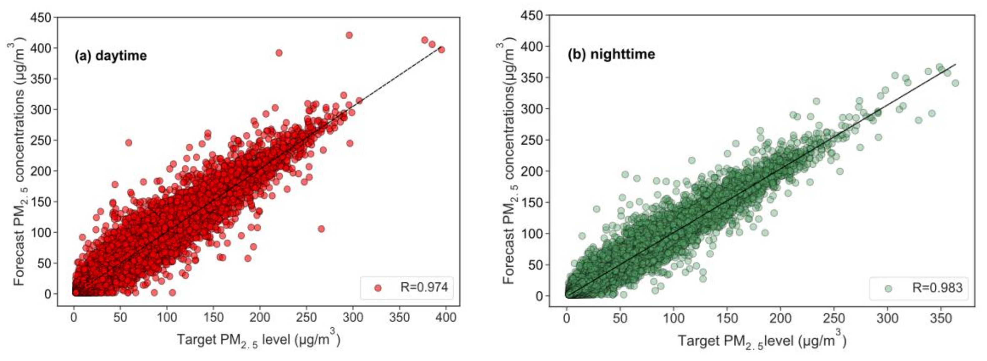
3.3. Comparison of Daytime and Nighttime Forecast Performance

Figure S2 shows that PM2.5 pollution patterns in cities with relatively high pollution are obviously different during the daytime and nighttime. Compared with the concentration changes during the nighttime, the concentration changes during the daytime are generally more drastically, mainly due to various kinds of human activities and always changing meteorological conditions during the daytime. This makes us wonder if there is any difference in forecast performance of PM2.5 between the daytime and the nighttime. We assume the time period of 7:00 a.m–8:00 p.m. as the daytime and the other time period as the nighttime. The comparison of the forecast performance of hourly PM2.5 concentration in one-hour advance for all cities in the YRD region during the daytime and nighttime periods is shown in Figure 4. In general, the forecast performance of the OR-ELM-AR model shows good stability. Both R values during daytime and nighttime are higher than 0.97. Furthermore, the R-value in the nighttime reaches 0.983, higher than in the daytime, because there are more affecting factors during the daytime. The concentration fluctuation in the daytime is relatively large, with a few samples close to 400 μg/m3.

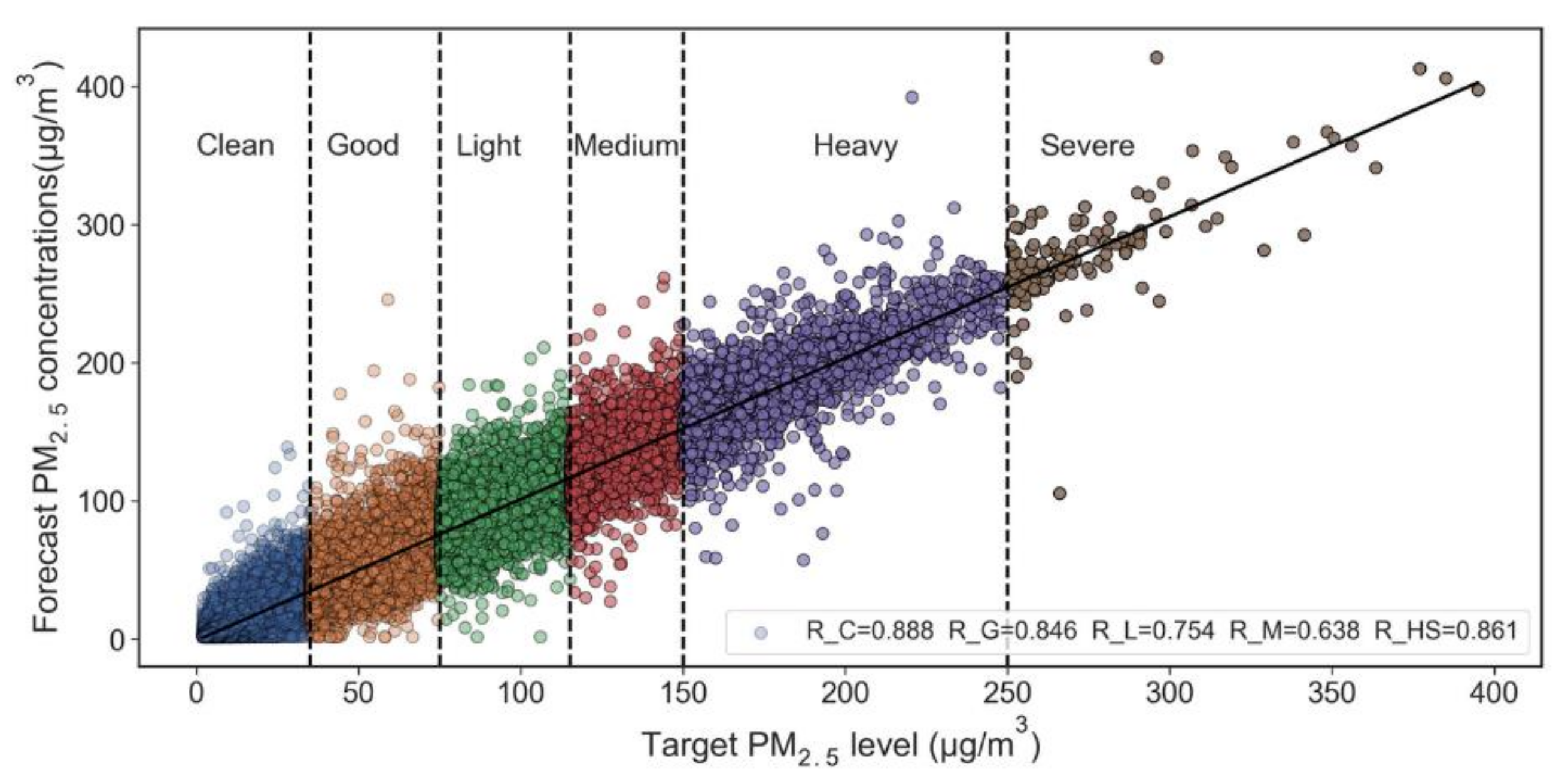
3.4. Forecast Performance at Different Pollution Levels

According to the technical regulations of the ambient air quality index (HJ 633–2012) issued by China government, air quality situations are classified into six categories: excellent, good, light, moderate, heavy and severe pollution. We evaluated the forecast performance at different pollution levels. Here, we combined heavy pollution and severe pollution into one group for forecast performance evaluation due to the limited number of severe pollution days. Generally, the forecast concentrations of the OR-ELM-AR algorithm were close to the target values for all pollution levels, as shown in Figure 5. From good to moderate pollution level, the R coefficient gradually decreased from 0.888 to 0.638 and then rose to 0.861 under heavy and severe conditions (Figure 5). This shows that the OR-ELM-AR model has slightly better adaptability at low and high levels of PM2.5 concentration compared with the intermediate pollution level.

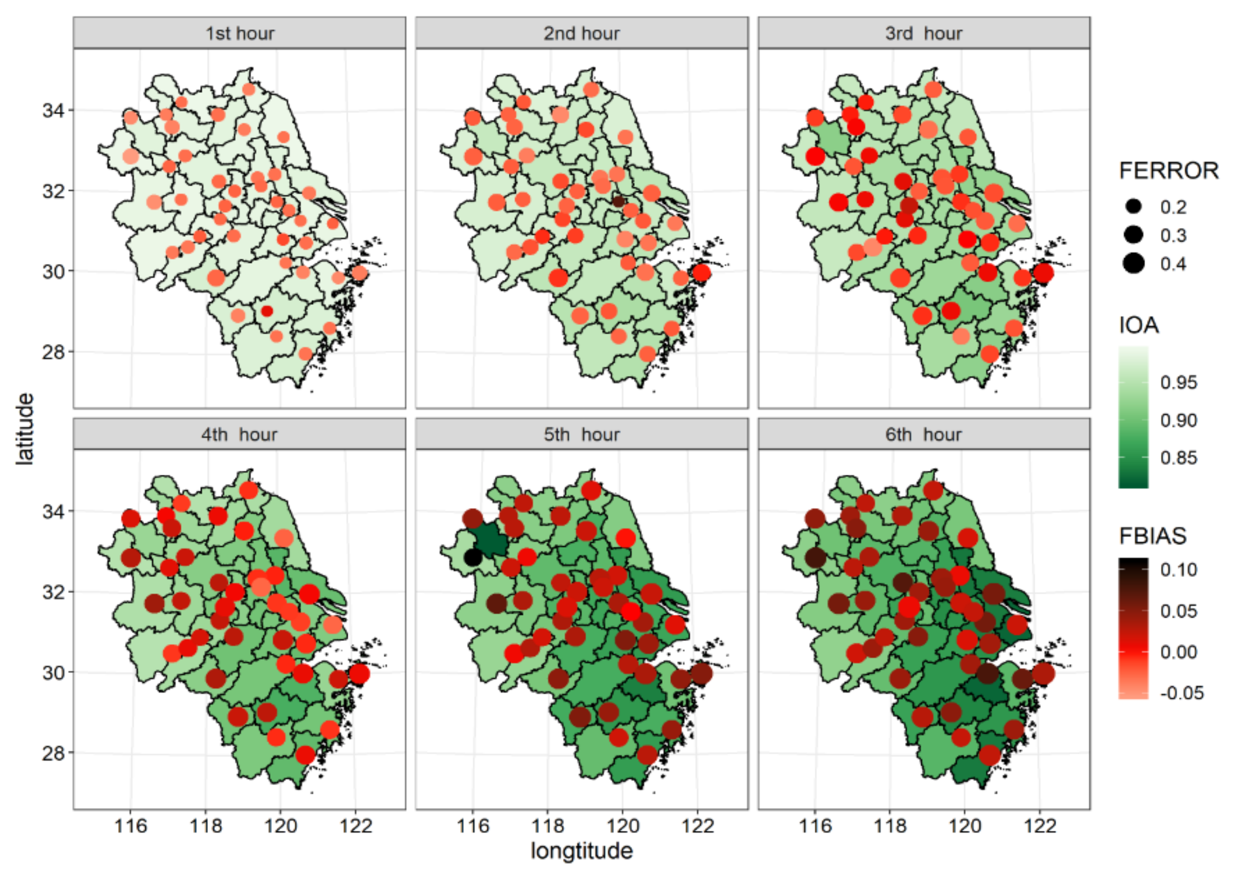
3.5. Spatial Forecast Performance

The forecast performance of the OR-ELM-AR model for hourly PM2.5 concentration forecast over the whole YRD region during 2019 is shown in Figure 6. The size of the circle represents the FERROR value. The color of the circle represents the FBIAS value, and the color in the map of the whole city area represents the IOA value of the corresponding city. Based on these, the figure reflects the variations of FBIAS, FERROR and IOA in the six sub-Figures with the forecast times and cities.
With the variation of forecast time from the first hour in advance to the sixth hour in advance, the FERROR values for all cities in the YRD region increase while the IOA values decrease gradually, suggesting that the performance of this model compromised when the forecast time gets longer. In contrast, the FBIAS value has the smallest fluctuation across cities and forecast times. Distinct differences of performance exist among these cities over the YRD region [29,30,31,32].
As shown in Figure 1, heavy pollution occurred in the north part of the YRD region, while the least polluted areas are located in the southern and western YRD region, as well as in Zhoushan city in the east of the YRD region. Combined with the spatial distribution of IOA, as shown in Figure 6, IOA values of areas with both the lowest and the highest PM2.5 concentration are obviously higher than those of the other areas. This is consistent with the previous result that the OR-ELM-AR model has better adaptability at low and high levels of PM2.5 concentration than that in middle levels. In addition, it also shows that the forecast performance weakens with the increase of the forecast time in advance based on the spatial distribution of forecast performance in the whole YRD region [32,33,34].
Figure 7 depicts the boxplots of forecast performance indicators varying with forecast times for all cities in the YRD region. The x-axis is the forecast time, and each sub-graph displays one evaluation indicator. As the forecast time becomes longer, the values of FBIAS, FERROR, BIAS, MAE and RMSE gradually increase, while the values of IOA and R gradually decrease. This shows that the overall forecast performance of the OR-ELM-AR model decreases slowly with the increase in the forecast time. The fluctuation range of performance indicators among these cities becomes larger gradually, suggesting that the performances among these cities become more heterogeneous. Compared with other indicators, the FEEROR value has the smallest fluctuation range. For FBIAS values, most of them fall in the narrow range from −0.05 to 0.05, mainly due to the inclusion of random algorithms in the OR-ELM-AR model.
As shown in Figure 8, the trends of all indicators with the pollution levels are similar under different forecast times. For a certain forecast time, FERROR values decrease slightly with the increase of PM2.5 pollution levels, while Bias, MAE, and RMSE, show upward trends with pollution levels, partially because PM2.5 concentration can amplify the values of these indicators. IOA and R have similar trends, where the forecast performance of OR-ELM-AR decreases gradually at first and then increases with the increase in pollution level. This indicates that the forecast performance is relatively low based on IOA and R evaluations in the middle pollution levels, which is consistent with the analysis from Figure 5. However, the lowest performance does not occur at the same pollution levels for different forecast times based on IOA and R evaluations. Compared with the lowest values of IOA and R for the other forecast times, the lowest values of IOA and R for the forecast at 1st hour in advance occur at the interval of a higher concentration of PM2.5. The forecast at the sixth hour in advance has the lowest performance at the concentration interval of [35, 75], after which performance becomes better as indicated by the IOA and R values, as shown in Figure 8. Moreover, the performance of the forecast at the first-hour advance is much better than that of the forecast at the sixth hour in advance in terms of any indicator among them.

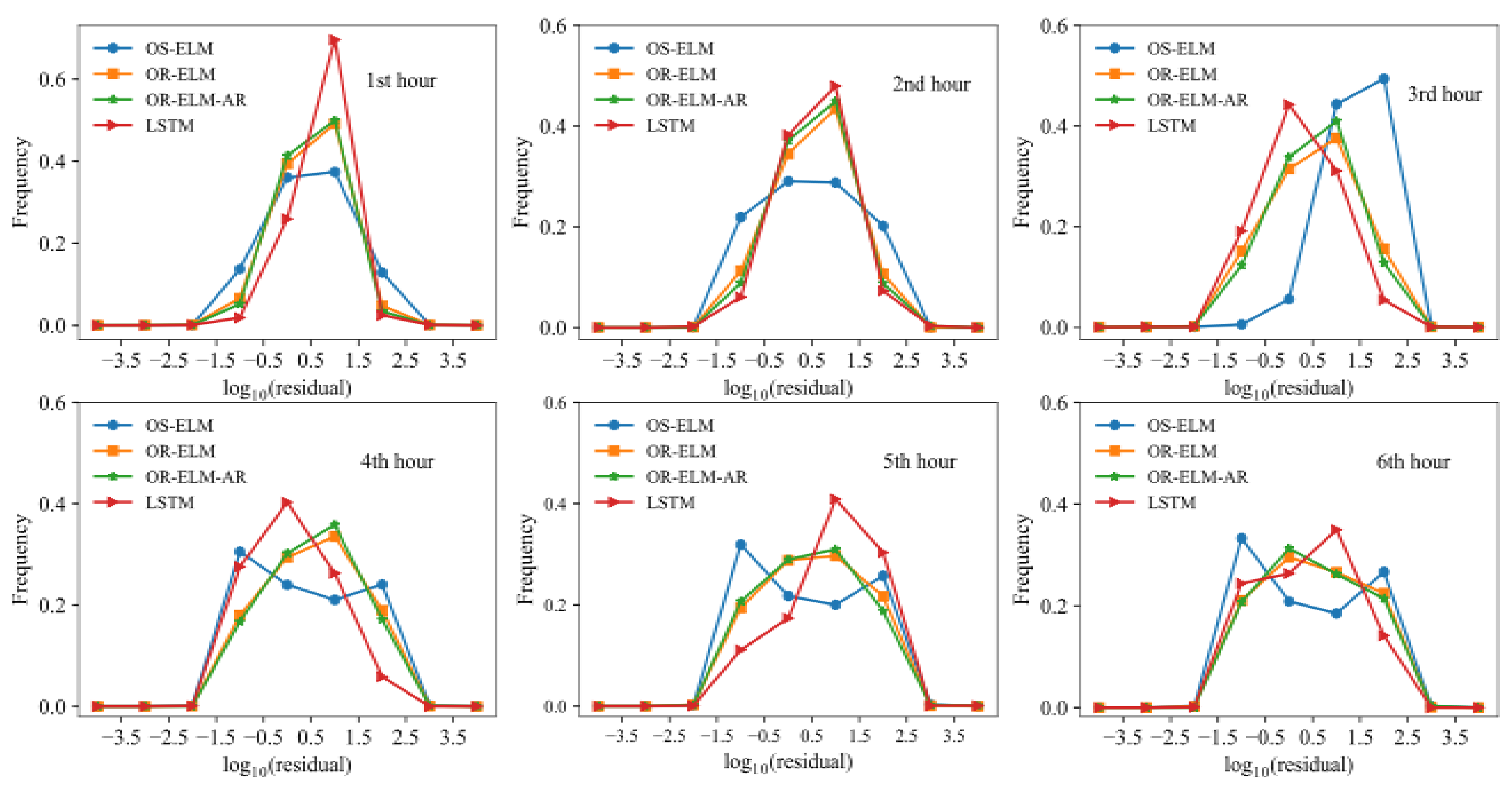
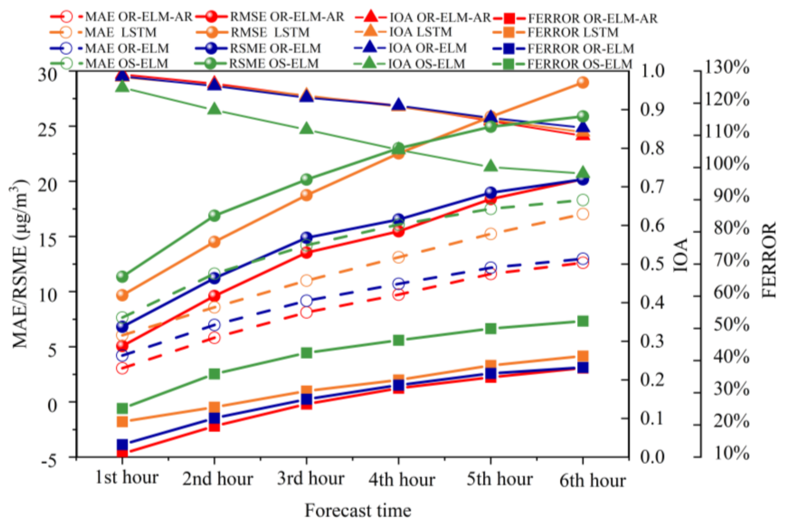
3.6. Comparison with Other Models

The forecasts of OR-ELM and OR-ELM-AR respond more quickly and have narrow deviations than that of OS-ELM both in high concentrations and low concentrations, as shown in Figure S3.
According to the forecast of hourly PM2.5 concentrations in the whole year 2019, the residuals of forecast in the first hour and second hour in advance show bell-shaped distributions and the results are relatively concentrated and stable, as shown in Figure 9. However, starting from the third hour in advance, OS-ELM′s residuals show bimodal distributions with large deviations. In addition, the residuals of LSTM expand with the increase in forecast time [35]. The skewness coefficients of LSTM′s residuals in the fourth, fifth and sixth hours in advance are 0.4652, −0.7803, and −0.026, respectively, exhibiting significant positive-skewed or negative-skewed. The OR-ELM-AR algorithm has residuals with near-zero skewness coefficients of −0.1235, 0.0288, and 0.0732 at the same forecast time, showing a more stable forecast with much smaller skewness.
Compared with the other three algorithms, the IOA values of OS-ELM are much lower, but the MAE, RMSE and FERROR values are much higher, as shown in Figure 10. The LSTM, OR-ELM and OR-ELM-AR models have similar IOA values as well as their FERROR values. Admittedly, the FERROR values of OR-LEM-AR are still the lowest. Both RMSE and MAE values of LSTM are much larger than those of OR-ELM-AR, with the forecast times varying from 1st hour to 6th hour in advance, suggesting the OR-ELM-AR algorithm has a much better ability of quickly responding to the short-term change than the LSTM algorithm.

4. Conclusions

In this work, online recurrent extreme learning machine (OR-ELM) was used to forecast hourly PM2.5 concentration for the first time. The hybrid model (OR-ELM-AR) was developed based on the OR-ELM model, coupled with the AR model. The performance of the OR-ELM-AR model in the forecast of hourly PM2.5 concentration was evaluated in detail over the YRD region in China. The main conclusions are as follows:
(1)
The PM2.5 forecast ability of OR-ELM-AR at nighttime is slightly better than that of daytime, mainly due to several influencing factors, such as more man-made sources and more changeable meteorological conditions in the daytime;
(2)
OR-ELM-AR model has better forecast performance for low and high levels of PM2.5 pollution than that for intermediate pollution levels. Especially in the cases of heavy and extreme heavy pollution, this model can respond to large temporal variations in concentration in time, with a higher correlation coefficient between the forecast values with the observed values. Compared with the intermediate polluted cities in the center part of the YRD region, the forecast performance is better for cities in the north part with heaviest pollution and cities in the southern and western part with the least pollution in the YRD region;
(3)
The OR-ELM-AR model gains much smaller RMSE and MAE values and slightly smaller FERROR values than the OR-ELM model by the embedded AR algorithm. The OS-ELM model has the worst forecast performance;
(4)
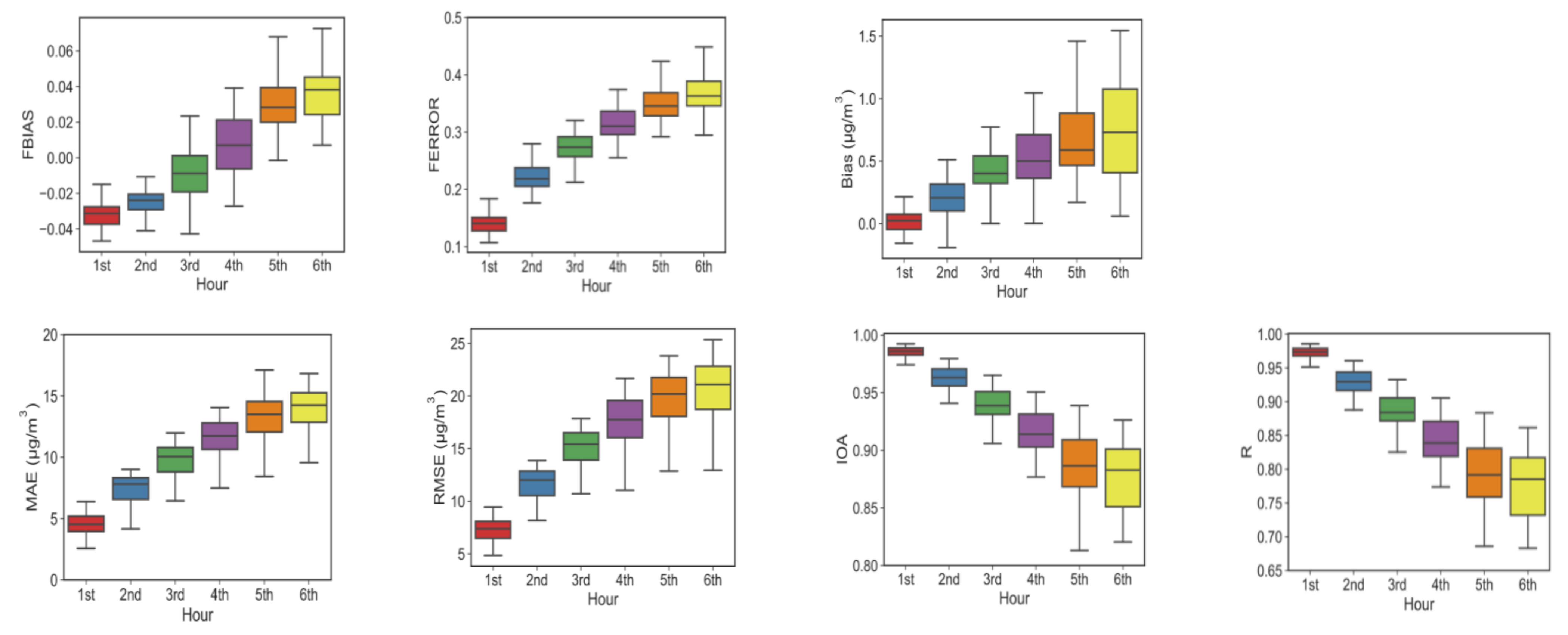
The OR-ELM-AR model has a much better ability of quick response than the LSTM model based on both RMSE and MAE metrics with the forecast times varying from 1st hour to 6th hour in advance, although their IOA values are close.
Overall, the OR-ELM-AR model is a promising tool of the short-term forecast of PM2.5 pollution to help the government take urgent action to reduce the occurrence rate and level of haze pollution in cities or regions.

Supplementary Materials

The following are available online at https://www.mdpi.com/2073-4433/12/1/78/s1, Figure S1: Variations of moving average PM2.5 concentrations of 20 weeks with time, Figure S2: Diurnal variation of the average concentrations of observed PM2.5 in the whole YRD(a) region, and Shanghai(b), Nanjing(c), Hangzhou(d), Heifei(e) and Xuzhou(f), respectively. Figure S3: Prediction of OS-ELM, OR-ELM and OR-ELM-AR with different lead times. All authors have read and agreed to the published version of the manuscript.

Author Contributions

Conceptualization and writing, Y.W.; methodology and writing, G.L.; visualization, E.Y., H.L. and Z.L.; writing, D.C.; editing, L.H. and K.M.; conceptualization, L.L. All authors have read and agreed to the published version of the manuscript.

Funding

This work was supported by the National Key R&D Program of China (No.2018YFC0213600), State Environmental Protection Key Laboratory of Sources and Control of Air Pollution Complex of China (SCAPC202003), the Shanghai Science and Technology Innovation Plan (NO.19DZ1205007), the Shanghai Sail Program (NO. 19YF1415600), and the National Natural Science Foundation of China (NO. 41875161).

Data Availability Statement

Not applicable.

Acknowledgments

We appreciate the High-Performance Computing Center of Shanghai University and Shanghai Engineering Research Center of Intelligent Computing System (No. 19DZ2252600) for providing the computing resources and technical support.

Conflicts of Interest

The authors declare that they have no known competing financial interests or personal relationships that could have appeared to influence the work reported in this paper.

References

  1. Chang, X.; Wang, S.; Zhao, B.; Xing, J.; Liu, X.; Wei, L.; Song, Y.; Wu, W.; Cai, S.; Zheng, H.; et al. Contributions of inter-city and regional transport to PM2.5 concentrations in the Beijing-Tianjin-Hebei region and its implications on regional joint air pollution control. Sci. Total Environ. 2019, 660, 1191–1200. [Google Scholar] [CrossRef]
  2. Cheng, N.; Zhang, D.; Li, Y.; Xie, X.; Chen, Z.; Meng, F.; Gao, B.; He, B. Spatio-temporal variations of PM2.5 concentrations and the evaluation of emission reduction measures during two red air pollution alerts in Beijing. Sci. Rep. 2017, 7, 8220. [Google Scholar] [CrossRef] [Green Version]
  3. Huang, L.; An, J.; Koo, B.; Yarwood, G.; Yan, R.; Wang, Y.; Huang, C.; Li, L. Sulfate formation during heavy winter haze events and the potential contribution from heterogeneous SO2 + NO2 reactions in the Yangtze River Delta region, China. Atmos. Chem. Phys. 2019, 19, 14311–14328. [Google Scholar] [CrossRef] [Green Version]
  4. Li, K.; Jacob, D.J.; Liao, H.; Zhu, J.; Shah, V.; Shen, L.; Bates, K.H.; Zhang, Q.; Zhai, S. A two-pollutant strategy for improving ozone and particulate air quality in China. Nat. Geosci. 2019, 12, 906–910. [Google Scholar] [CrossRef]
  5. Kan, H.; Chen, R.; Tong, S. Ambient air pollution, climate change, and population health in China. Environ. Int. 2012, 42, 10–19. [Google Scholar] [CrossRef] [PubMed]
  6. Li, Z.; Wang, Y.; Guo, J.; Zhao, C.; Cribb, M.C.; Dong, X.; Fan, J.; Gong, D.; Huang, J.; Jiang, M.; et al. East Asian Study of Tropospheric Aerosols and their Impact on Regional Clouds, Precipitation, and Climate (EAST-AIR CPC). J. Geophys. Res. Atmos. 2019, 124, 13026–13054. [Google Scholar] [CrossRef] [Green Version]
  7. Lin, H.; Ma, W.; Qiu, H.; Wang, X.; Trevathan, E.; Yao, Z.; Dong, G.H.; Vaughn, M.G.; Qian, Z.; Tian, L. Using daily excessive concentration hours to explore the short-term mortality effects of ambient PM2.5 in Hong Kong. Environ. Pollut. 2017, 229, 896–901. [Google Scholar] [CrossRef] [PubMed] [Green Version]
  8. Huang, C.J.; Kuo, P.H. A Deep CNN-LSTM Model for Particulate Matter (PM2.5) Forecasting in Smart Cities. Sensors (Basel) 2018, 18, 2220. [Google Scholar] [CrossRef] [Green Version]
  9. Wang, Y.; Bao, S.; Wang, S.; Hu, Y.; Shi, X.; Wang, J.; Zhao, B.; Jiang, J.; Zheng, M.; Wu, M.; et al. Local and regional contributions to fine particulate matter in Beijing during heavy haze episodes. Sci. Total Environ. 2017, 580, 283–296. [Google Scholar] [CrossRef]
  10. Zheng, B.; Zhang, Q.; Zhang, Y.; He, K.B.; Wang, K.; Zheng, G.J.; Duan, F.K.; Ma, Y.L.; Kimoto, T. Heterogeneous chemistry: A mechanism missing in current models to explain secondary inorganic aerosol formation during the January 2013 haze episode in North China. Atmos. Chem. Phys. 2015, 15, 2031–2049. [Google Scholar] [CrossRef] [Green Version]
  11. Liu, D.; Sun, K. Short-term PM2.5 forecasting based on CEEMD-RF in five cities of China. Environ. Sci. Pollut. Res. Int. 2019, 26, 32790–32803. [Google Scholar] [CrossRef]
  12. Feng, X.; Li, Q.; Zhu, Y.; Hou, J.; Jin, L.; Wang, J. Artificial neural networks forecasting of PM2.5 pollution using air mass trajectory based geographic model and wavelet transformation. Atmos. Environ. 2015, 107, 118–128. [Google Scholar] [CrossRef]
  13. Wang, D.; Wei, S.; Luo, H.; Yue, C.; Grunder, O. A novel hybrid model for air quality index forecasting based on two-phase decomposition technique and modified extreme learning machine. Sci. Total Environ. 2017, 580, 719–733. [Google Scholar] [CrossRef] [PubMed]
  14. Park, J.-M.; Kim, J.-H. Online recurrent extreme learning machine and its application to time-series prediction. In Proceedings of the International Joint Conference on Neural Networks (IJCNN) 2017, Anchorage, AK, USA, 14–19 May 2017; pp. 1983–1990. [Google Scholar] [CrossRef]
  15. Marsha, A.; Larkin, N.K. A statistical model for predicting PM2.5 for the western United States. J. Air Waste Manag. Assoc. 2019, 69, 1215–1229. [Google Scholar] [CrossRef] [PubMed]
  16. Feng, R.; Zheng, H.-J.; Gao, H.; Zhang, A.-R.; Huang, C.; Zhang, J.-X.; Luo, K.; Fan, J.-R. Recurrent Neural Network and random forest for analysis and accurate forecast of atmospheric pollutants: A case study in Hangzhou, China. J. Clean. Product. 2019, 231, 1005–1015. [Google Scholar] [CrossRef]
  17. Mao, X.; Shen, T.; Feng, X. Prediction of hourly ground-level PM2.5 concentrations 3 days in advance using neural networks with satellite data in eastern China. Atmos. Pollut. Res. 2017, 8, 1005–1015. [Google Scholar] [CrossRef]
  18. Gao, S.; Huang, Y.; Zhang, S.; Han, J.; Wang, G.; Zhang, M.; Lin, Q. Short-term runoff prediction with GRU and LSTM networks without requiring time step optimization during sample generation. J. Hydrol. 2020, 589, 125188. [Google Scholar] [CrossRef]
  19. Díaz-Robles, L.A.; Ortega, J.C.; Fu, J.S.; Reed, G.D.; Chow, J.C.; Watson, J.G.; Moncada-Herrera, J.A. A hybrid ARIMA and artificial neural networks model to forecast particulate matter in urban areas: The case of Temuco, Chile. Atmos. Environ. 2008, 42, 8331–8340. [Google Scholar] [CrossRef] [Green Version]
  20. Zhou, Q.; Jiang, H.; Wang, J.; Zhou, J. A hybrid model for PM(2).(5) forecasting based on ensemble empirical mode decomposition and a general regression neural network. Sci. Total Environ. 2014, 496, 264–274. [Google Scholar] [CrossRef]
  21. Murray, N.L.; Holmes, H.A.; Liu, Y.; Chang, H.H. A Bayesian ensemble approach to combine PM2.5 estimates from statistical models using satellite imagery and numerical model simulation. Environ. Res. 2019, 178, 108601. [Google Scholar] [CrossRef]
  22. Yu, L.; Dai, W.; Tang, L. A novel decomposition ensemble model with extended extreme learning machine for crude oil price forecasting. Eng. Appl. Artif. Intell. 2016, 47, 110–121. [Google Scholar] [CrossRef]
  23. Zhang, N.N.; Ma, F.; Qin, C.B.; Li, Y.F. Spatiotemporal trends in PM2.5 levels from 2013 to 2017 and regional demarcations for joint prevention and control of atmospheric pollution in China. Chemosphere 2018, 210, 1176–1184. [Google Scholar] [CrossRef] [PubMed]
  24. Liu, B.; Yan, S.; Li, J.; Qu, G.; Li, Y.; Lang, J.; Gu, R. A Sequence-to-Sequence Air Quality Predictor Based on the n-Step Recurrent Prediction. IEEE Access 2019, 7, 43331–43345. [Google Scholar] [CrossRef]
  25. Bueno, A.; Coelho, G.P.; Bertini, J.R. Online sequential learning based on extreme learning machines for particulate matter forecasting. In Proceedings of the 2017 Brazilian Conference on Intelligent Systems (BRACIS), Uberlandia, Brazil, 2–5 October 2017; pp. 169–174. [Google Scholar] [CrossRef]
  26. Huang, G.; Liang, N.; Rong, H.; Saratchandran, P.; Sundararajan, N. On-line sequential extreme learning machine. In Proceedings of the IASTED International Conference on Computational Intelligence, Calgary, AB, Canada, 4–6 July 2005. [Google Scholar]
  27. Liu, H.; Xu, Y.; Chen, C. Improved pollution forecasting hybrid algorithms based on the ensemble method. Appl. Math. Model. 2019, 73, 473–486. [Google Scholar] [CrossRef]
  28. James, J. Robustness of simple trend-following strategies. Quant. Financ. 2003, 3, C114–C116. [Google Scholar] [CrossRef]
  29. Kanada, M.; Dong, L.; Fujita, T.; Fujii, M.; Inoue, T.; Hirano, Y.; Togawa, T.; Geng, Y. Regional disparity and cost-effective SO2 pollution control in China: A case study in 5 mega-cities. Energy Policy 2013, 61, 1322–1331. [Google Scholar] [CrossRef]
  30. Li, J.; Du, H.; Wang, Z.; Sun, Y.; Yang, W.; Li, J.; Tang, X.; Fu, P. Rapid formation of a severe regional winter haze episode over a mega-city cluster on the North China Plain. Environ. Pollut. 2017, 223, 605–615. [Google Scholar] [CrossRef]
  31. Wang, Q.; Kwan, M.P.; Zhou, K.; Fan, J.; Wang, Y.; Zhan, D. The impacts of urbanization on fine particulate matter (PM2.5) concentrations: Empirical evidence from 135 countries worldwide. Environ. Pollut. 2019, 247, 989–998. [Google Scholar] [CrossRef]
  32. Zhai, S.; Jacob, D.J.; Wang, X.; Shen, L.; Li, K.; Zhang, Y.; Gui, K.; Zhao, T.; Liao, H. Fine particulate matter (PM2.5) trends in China, 2013–2018: Separating contributions from anthropogenic emissions and meteorology. Atmos. Chem. Phys. 2019, 19, 11031–11041. [Google Scholar] [CrossRef] [Green Version]
  33. Zhang, Q.; Quan, J.; Tie, X.; Li, X.; Liu, Q.; Gao, Y.; Zhao, D. Effects of meteorology and secondary particle formation on visibility during heavy haze events in Beijing, China. Sci. Total Environ. 2015, 502, 578–584. [Google Scholar] [CrossRef]
  34. Zhao, B.; Wang, S.; Ding, D.; Wu, W.; Chang, X.; Wang, J.; Xing, J.; Jang, C.; Fu, J.S.; Zhu, Y.; et al. Nonlinear relationships between air pollutant emissions and PM2.5-related health impacts in the Beijing-Tianjin-Hebei region. Sci. Total Environ. 2019, 661, 375–385. [Google Scholar] [CrossRef] [PubMed]
  35. Zhao, J.; Deng, F.; Cai, Y.; Chen, J. Long short-term memory-Fully connected (LSTM-FC) neural network for PM2.5 concentration prediction. Chemosphere 2019, 220, 486–492. [Google Scholar] [CrossRef] [PubMed]
Figure 1. Geographic location of the Yangtze River Delta region and its prefecture-level cities.
Atmosphere 12 00078 g001
Figure 2. The main framework of the hybrid machine learning method (OR-ELM-AR) model.
Atmosphere 12 00078 g002
Figure 3. The performance variations with neuron number (left) and the length of input sample length (right).
Atmosphere 12 00078 g003
Figure 4. Scatter plots of forecasted and target fine particulate matter (PM2.5) concentrations based on the OR-ELM-AR during the daytime (a) and during the nighttime (b).
Atmosphere 12 00078 g004
Figure 5. Comparison of forecast results and targets in different pollution levels.
Atmosphere 12 00078 g005
Figure 6. Distributions of fractional bias (FBIAS), fractional error (FERROR) and index of agreement (IOA) over cities with the variation of forecast times.
Atmosphere 12 00078 g006
Figure 7. Boxplot of performance indicators with different forecast times.
Atmosphere 12 00078 g007
Figure 8. Forecast performance of the OR-ELM-AR model under different pollution levels.
Atmosphere 12 00078 g008
Figure 9. Residual distributions of the extreme learning machine (OS-ELM), online recurrent extreme learning machine (OR-ELM), OR-ELM-AR and LSTM models.
Atmosphere 12 00078 g009
Figure 10. Comparison of forecast performance for four models.
Atmosphere 12 00078 g010
Table 1. Statistical measures of evaluation of forecast performance.
StatisticDefinitionNotes
Mean error (bias) B i a s = 1 N ( M i O i ) Concentration units
Mean absolute error (MAE) M A E = 1 N | M i O i | Concentration units
Root-mean-squared error (RMSE) R M S E = 1 N ( M i O i ) 2 Concentration units
Index of agreement (IOA) I O A = 1 ( M i O i ) 2 | M i O ¯ i | + | O i O ¯ i | 2 Unitless, 0 ≤ IOA ≤ 1
Fractional bias (FBIAS) F B I A S = 2 N ( M i O i ) ( M i + O i ) −2 ≤ FBIAS ≤ 2
Fractional error (FERROR) F E R R O R = 2 N | M i O i | ( M i + O i ) 0 ≤ FERROR ≤ 2
Correlation (R) c o r r = ( M i M ¯ i ) ( O i O ¯ i ) ( M i M ¯ i ) 2 ( O i O ¯ i ) 2 −1 ≤ corr ≤ 1
Note. Subscript j represents the pairing of N observations M and predictions P by the time. Overbars signify means over time.
Publisher’s Note: MDPI stays neutral with regard to jurisdictional claims in published maps and institutional affiliations.

