Characterization of PM10 Sampled on the Top of a Former Mining Tower by the High-Volume Wind Direction-Dependent Sampler Using INNA

 , , ,
, , ,
Abstract
1. Introduction
2. Experiments
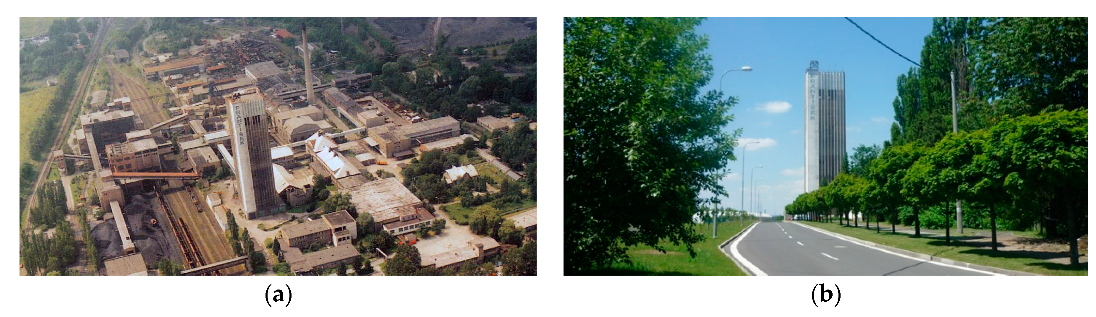
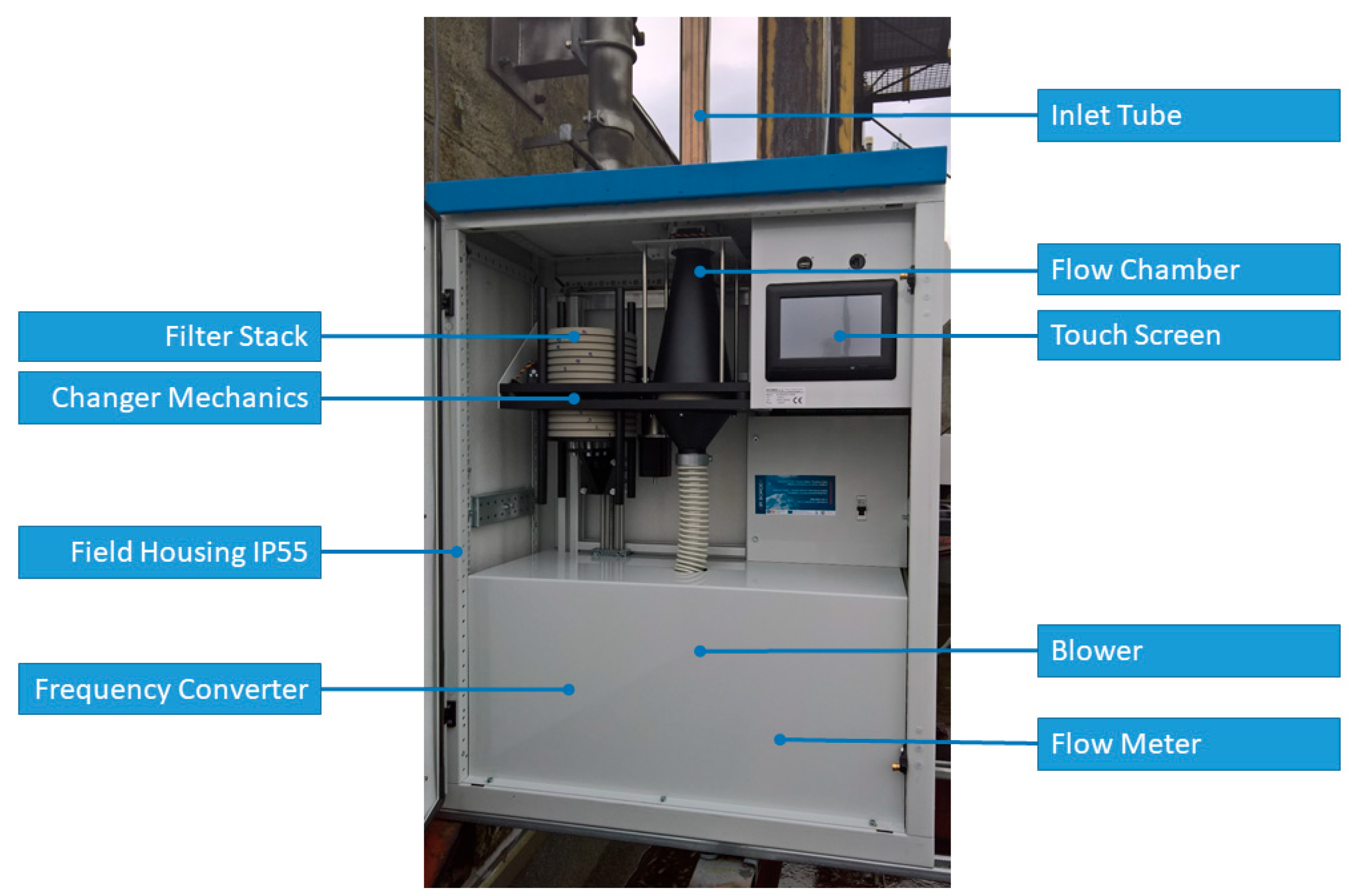
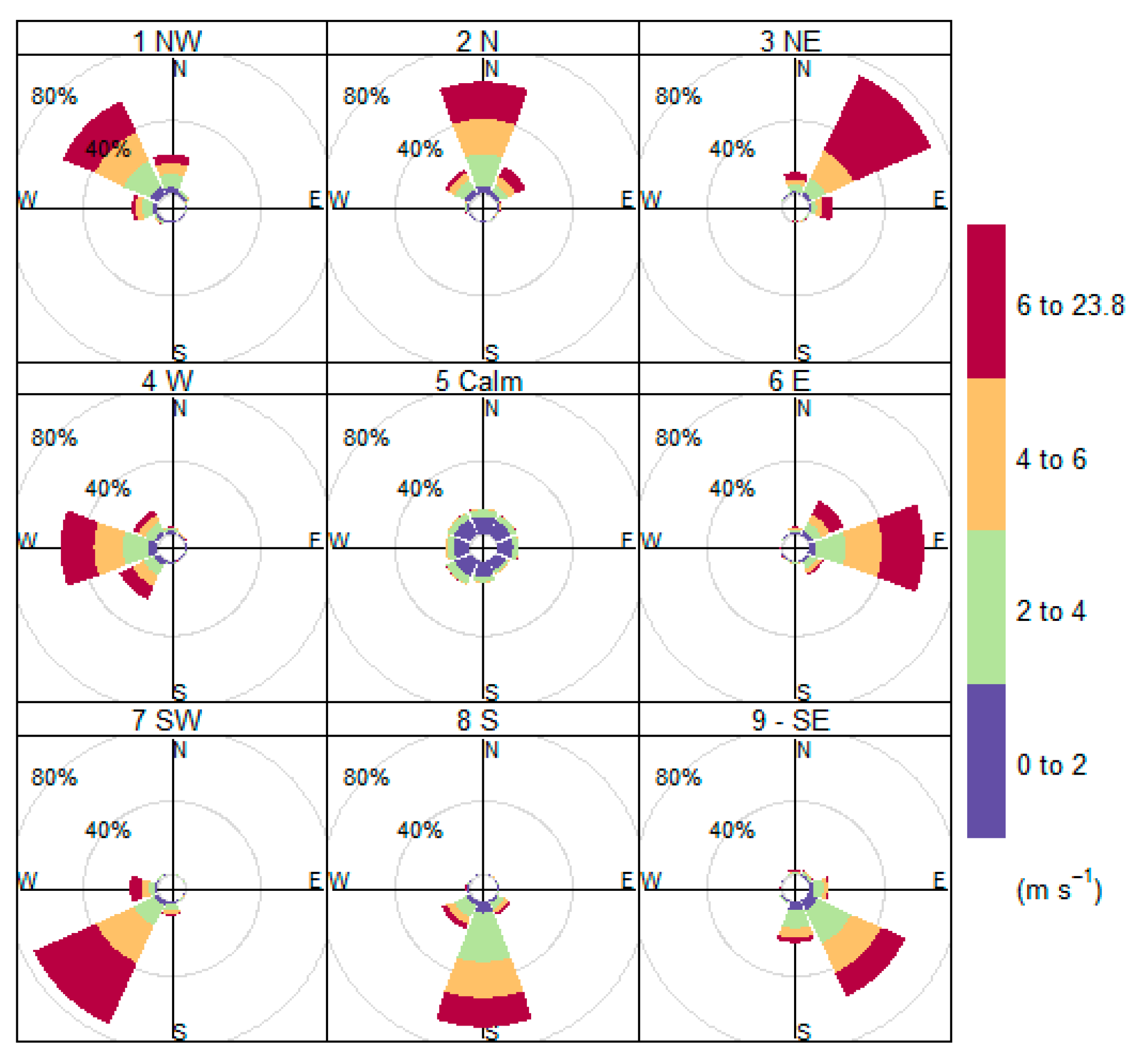
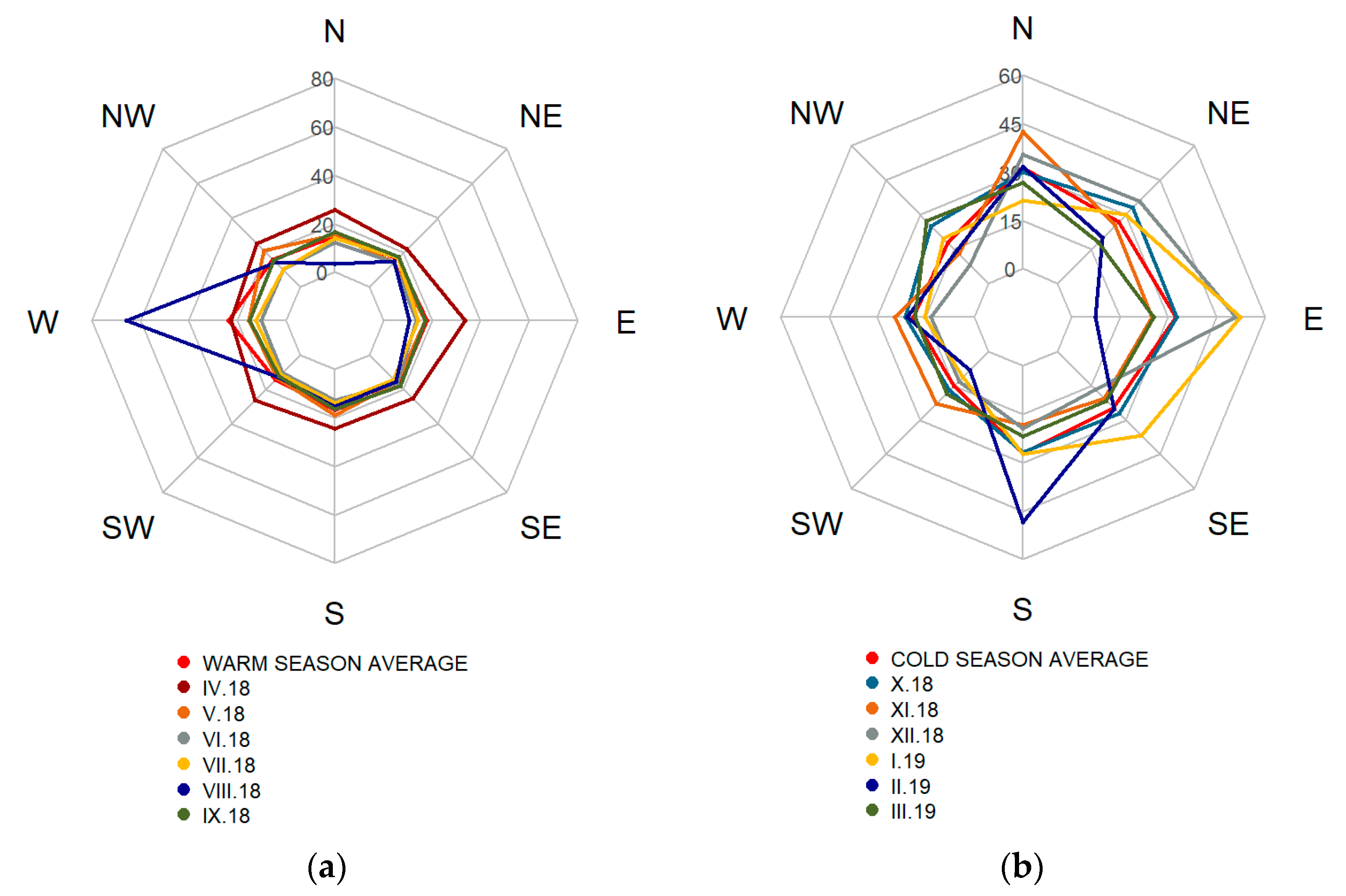
2.1. Sampling
2.2. Determination of PM10 Mass Concentrations
2.3. Element Content Determination Using Neutron Activation Analysis
2.4. Statistical Analyses and Visualization
3. Results
3.1. PM10 Mass Concentrations
3.2. Element Content Characterization
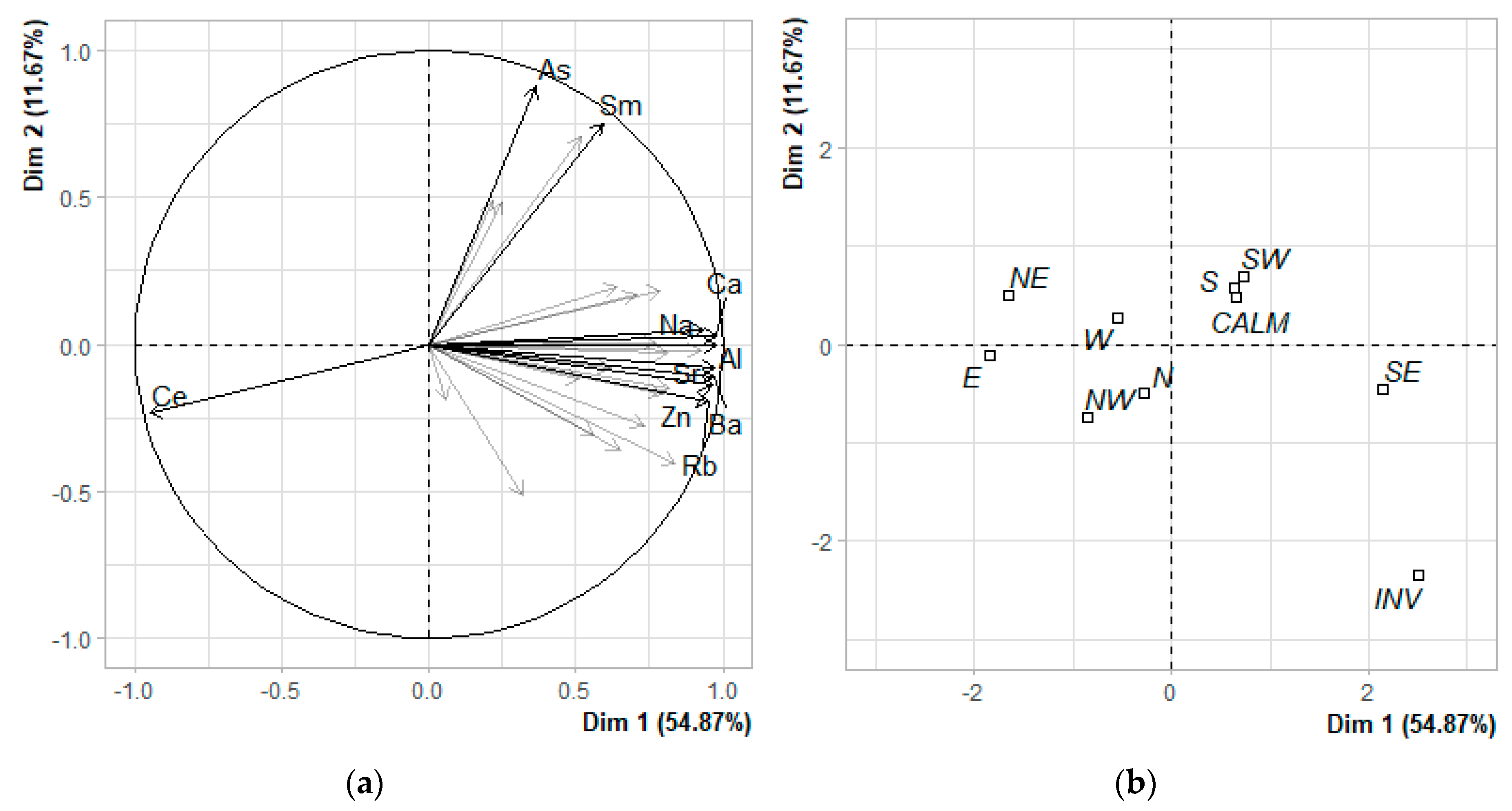
3.3. Principal Component Analysis (PCA)
3.3.1. PCA of The Warm Season Measurements
3.3.2. PCA of the Cold Season Measurements
4. Discussion
5. Conclusions
Supplementary Materials
Author Contributions
Funding
Data Availability Statement
Acknowledgments
Conflicts of Interest
References
- Klusácek, P. Downsizing of bituminous coal mining and the restructuring of steel works and heavy machine engineering in the Ostrava region. Moriv. Geogr. Rep. 2005, 13, 3–11. [Google Scholar]
- Cabala, J.; Cmiel, S.R.; Idziak, A.F. Environmental impact of mining activity in the upper silesian coal basin. Geol. Belg. 2004, 7, 225–229. [Google Scholar]
- Blažek, Z.; Černikovsky, L.; Krejči, B.; Osrodka, L.; Volna, V.; Wojtylak, M. Vliv Meteorologických Podmínek Na Kvalitu Ovzduší V Přeshraniční Oblasti Slezska A Moravy—Wpływ Warunków Meteoro-Logicznych Na Jakość Powietrza W Obszarze Przygranicznym Śląska I Moraw [The Influence of Meteorological Conditions on Air Quality in the Border Region of Silesia and Moravia], 1st ed.; Český Hydrometeorologický Ústav: Prague, Czech Republic; Instytut Meteorologii i Gospodarki Wodnej, Państwowy Instytut Badawczy: Warsaw, Poland, 2013; ISBN 978-80-87577-15-8. (In Czech/Polish). [Google Scholar]
- Hůnová, I. Ambient air quality in the Czech Republic: Past and present. Atmosphere 2020, 11, 214. [Google Scholar] [CrossRef]
- Kuskova, P.; Gingrich, S.; Krausmann, F. Long term changes in social metabolism and land use in Czechoslovakia, 1830–2000: An energy transition under changing political regimes. Ecol. Econ. 2008, 68, 394–407. [Google Scholar] [CrossRef]
- Ďurčanská, D.; Drličiak, M.; Jandačka, D.; Bitta, J.; Bizek, V.; Foldynová, I.; Hladký, D.; Hrušková, A.; Hruška, L.; Chovanec, P.; et al. Riadenie Kvality Ovzdušia [Air Quality Management]; Žilinská Univerzita V Žiline—EDIS—Vydavate’ské Centrum ŽU: Žilina, Slovakia, 2020; ISBN 978-80-554-1658-8. (In Czech, Slovaque/Polish). [Google Scholar]
- Główny Urząd Statystyczny. Zużycie Energii w Gospodarstwach Domowych w 2018 Roku [Energy Consumption in Households in 2018]; Główny Urząd Statystyczny—Statistics Poland: Warsaw, Poland, 2019; Volume 2019. [Google Scholar]
- European Environment Agency. Air Quality in Europe—2019 Report; Number 10; European Environment Agency: Luxembourg, 2019; ISBN 978-92-9480-088-6.
- Czech Hydrometeorological Institute. Summary Tabular Survey. 2018. Available online: http://portal.chmi.cz/files/portal/docs/uoco/isko/tab_roc/2018_enh/index_GB.html (accessed on 14 April 2020).
- European Council. Directive 2008/50/EC of the European Parliament and of the Council of 21 May 2008 on Ambient Air Quality and Cleaner Air for Europe; OJEC L 152; European Council: Brussel, Belgium, 2008. [Google Scholar]
- World Health Organization. Air Quality Guidelines: Global Update 2005: Particulate Matter, Ozone, Nitrogen Dioxide, and Sulfur Dioxide; World Health Organization: Copenhagen, Denmark, 2006; ISBN 978-92-890-2192-0. [Google Scholar]
- WHO Regional Office for Europe. Evolution of WHO Air Quality Guidelines Past, Present and Future; WHO: Copenhagen, Denmark, 2017; ISBN 978-92-890-5230-6. [Google Scholar]
- Jiřík, V.; Hermanová, B.; Dalecká, A.; Pavlíková, I.; Bitta, J.; Jančík, P.; Ośródka, L.; Krajny, E.; Sładeczek, F.; Siemiątkowski, G.; et al. Wpływ Zanieczyszczenia Powietrza Na Zdrowie Ludności W Obszarze Polsko-Czeskiego Pogranicza. Dopad Znečištění Ovzduší Na Zdravotní Stav Obyvatelstva V Česko-Polském Příhraničí [Impact of Air Pollution on the Health Status of the Population in the Czech-Polish Border]; Sieć Badawcza Łukasiewicz—Instytut Ceramiki i Materiałów Budowlanych Instytut Meteorologii i Gospodarki Wodnej—Państwowy Instytut Badawczy Ostravská Univerzita Vysoká Škola Báňská—Technická Univerzita Ostrava: Ostrava, Czech Republic, 2020; ISBN 978-80-248-4406-0. (In Czech/Polish). [Google Scholar]
- World Health Organization. Ambient Air Pollution: A Global Assessment of Exposure and Burden of Disease; WHO: Geneva, Switzerland, 2016; ISBN 978-92-4-151135-3. [Google Scholar]
- World Health Organization. Review of Evidence on Health Aspects of Air Pollution—REVIHAAP Project; Technical Report; World Health Organization: Copenhagen, Denmark, 2013. [Google Scholar]
- Jiřík, V.; Machaczka, O.; Miturová, H.; Tomášek, I.; Šlachtová, H.; Janoutová, J.; Velická, H.; Janout, V. Air pollution and potential health risk in Ostrava region—A review. Cent. Eur. J. Public Health 2016, 24, S4–S17. [Google Scholar] [CrossRef] [PubMed]
- Cohen, A.; Samet, J.M.; Straif, K. (Eds.) Air Pollution and Cancer; International Agency for Research on Cancer: Lyon, France, 2013; Volume 161, ISBN 978-92-832-2161-6. [Google Scholar]
- The Czech Statistical Office. Czech Demographic Handbook—2018. Available online: https://www.czso.cz/csu/czso/czech-demographic-handbook (accessed on 29 June 2020).
- Pinto, J.P.; Stevens, R.K.; Willis, R.D.; Kellogg, R.; Mamane, Y.; Novak, J.; Šantroch, J.; Beneš, I.; Lenicek, J.; Bureš, V. Czech air quality monitoring and receptor modeling study. Environ. Sci. Technol. 1998, 32, 843–854. [Google Scholar] [CrossRef]
- Čížová, H. Projekt Slezsko/Silesia [The Silesia Project]. Zprav. Minist. Životn. Prostředí ČR 1994, 3, 6–7. (In Czech) [Google Scholar]
- Jančík, P.; Pavlíková, I.; Bitta, J.; Hladký, D. Atlas Ostravského Ovzduší; Vysoká Škola Báňská—Technická Univerzita Ostrava: Ostrava, Czech Republic, 2013; ISBN 978-80-248-3006-3. [Google Scholar]
- Air TRITIA—Uniform Approach to the Air Polution Management System for Functional Urban Areas in TRITIA Region. Available online: http://www.interreg-central.eu/Content.Node/AIR-TRITIA.html (accessed on 17 April 2020).
- Mikuška, P.; Křůmal, K.; Večeřa, Z. Characterization of organic compounds in the PM2.5 aerosols in winter in an industrial urban area. Atmos. Environ. 2015, 105, 97–108. [Google Scholar] [CrossRef]
- Pokorná, P.; Hovorka, J.; Klán, M.; Hopke, P.K. Source apportionment of size resolved particulate matter at a European air pollution hot spot. Sci. Total Environ. 2015, 502, 172–183. [Google Scholar] [CrossRef]
- Leoni, C.; Pokorná, P.; Hovorka, J.; Masiol, M.; Topinka, J.; Zhao, Y.; Křůmal, K.; Cliff, S.; Mikuška, P.; Hopke, P.K. Source apportionment of aerosol particles at a european Air Pollution hot spot using particle number size distributions and chemical composition. Environ. Pollut. Barking Essex 1987 2018, 234, 145–154. [Google Scholar] [CrossRef]
- Aglomerace Ostrava/Karviná/Frýdek-Místek. Český Hydrometeorologický Ústav Aktualizace Programů Zlepšovaní Kvality Ovzduší 2020+; Ministerstvo Životního Prostředí ČR: Prague, Czech Republic, 2019.
- Seibert, R.; Nikolova, I.; Volná, V.; Krejčí, B.; Hladký, D. Air pollution sources’ contribution to PM2.5 concentration in the northeastern part of the Czech Republic. Atmosphere 2020, 11, 522. [Google Scholar] [CrossRef]
- Czech Hydrometeorological Institute. Summary Tabular Survey. 2015. Available online: http://portal.chmi.cz/files/portal/docs/uoco/isko/tab_roc/2015_enh/index_GB.html (accessed on 23 April 2020).
- Černikovský, L.; Krejčí, B.; Blažek, Z.; Volná, V. Transboundary air-pollution transport in the Czech-Polish border region between the cities of Ostrava and Katowice. Cent. Eur. J. Public Health 2016, 24, S45–S50. [Google Scholar] [CrossRef] [PubMed]
- Volná, V.; Hladký, D. Detailed assessment of the effects of meteorological conditions on PM10 concentrations in the northeastern part of the Czech Republic. Atmosphere 2020, 11, 497. [Google Scholar] [CrossRef]
- U.S. Environmental Protection Agency. Compendium of Methods for the Determination of Inorganic Compounds in Ambient Air: Sampling of Ambient Air for Total Suspended Particulate Matter (Spm) and PM10 Using High Volume (Hv) Sampler; U.S. Environmental Protection Agency: Cincinnati, OH, USA, 1999.
- Krug, J.D.; Dart, A.; Witherspoon, C.L.; Gilberry, J.; Malloy, Q.; Kaushik, S.; Vanderpool, R.W. Revisiting the size selective performance of EPA’s high-volume total suspended particulate matter (Hi-Vol TSP) sampler. Aerosol. Sci. Technol. 2017, 51, 868–878. [Google Scholar] [CrossRef]
- European Committee for Standardization. Ambient Air. Standard Gravimetric Measurement Method for the Determination of the PM10 or PM2,5 Mass Concentration of Suspended Particulate Matter; EN 12341:2014; NSAI: Dublin, Ireland, 2014. [Google Scholar]
- U.S. Environmental Protection Agency. Office of Air and Radiation. Office of Air Quality Planning and Standards Meteorological Monitoring Guidance for Regulatory Modeling Applications; U.S. Environmental Protection Agency: Cincinnati, OH, USA, 2000.
- Frontasyeva, M.V.; Pavlov, S.S.; Shvetsov, V.N. NAA for applied investigations at FLNP JINR: Present and future. J. Radioanal. Nucl. Chem. 2010, 286, 519–524. [Google Scholar] [CrossRef]
- Pavlov, S.; Dmitriev, A.; Frontasyeva, M. Automation system for neutron activation analysis at the reactor IBR-2, Frank Laboratory of Neutron Physics, Joint Institute for Nuclear Research, Dubna, Russia. J. Radioanal. Nucl. Chem. 2016, 309, 27–38. [Google Scholar] [CrossRef]
- Dray, S.; Josse, J. Principal component analysis with missing values: A comparative survey of methods. Plant. Ecol. 2015, 216, 657–667. [Google Scholar] [CrossRef]
- Hron, K.; Templ, M.; Filzmoser, P. Imputation of missing values for compositional data using classical and robust methods. Comput. Stat. Data Anal. 2010, 54, 3095–3107. [Google Scholar] [CrossRef]
- U.S. Environmental Protection Agency. Compendium Method IO-3.7—Determination of Metals in Ambient Particulate Matter Using Neutron Activation Analysis (NAA) Gamma Spectrometry; U.S. Environmental Protection Agency: Cincinnati, OH, USA, 1999.
- The R Foundation. Available online: https://www.r-project.org/ (accessed on 25 December 2020).
- Lê, S.; Josse, J.; Husson, F. FactoMineR: An R package for multivariate analysis. J. Stat. Softw. 2008, 25. [Google Scholar] [CrossRef]
- Husson, F.; Josse, J.; Le, S.; Mazet, J. Package ‘FactoMineR’—Multivariate Exploratory Data Analysis and Data Mining. Available online: https://cran.r-project.org/web/packages/FactoMineR/index.html (accessed on 25 December 2020).
- Carslaw, D.; Ropkins, K. Package ‘Openair’—Tools for the Analysis of Air Pollution Data. Available online: https://davidcarslaw.github.io/openair/ (accessed on 25 December 2020).
- Wickham, H.; Chang, W.; Henry, L.; Pedersen, T.L.; Takahashi, K.; Wilke, C.; Woo, K.; Yutani, H.; Dunnington, D. Package ‘Ggplot2′—Create Elegant Data Visualisations Using the Grammar of Graphics. Available online: https://ggplot2.tidyverse.org/reference/ggplot2-package.html (accessed on 25 December 2020).
- Pawlowsky-Glahn, V.; Buccianti, A. (Eds.) Compositional Data Analysis: Theory and Applications; Wiley: Chichester, UK, 2011; ISBN 978-0-470-71135-4. [Google Scholar]
- Aitchison, J. The Statistical Analysis of Compositional Data; Blackburn Press: Caldwell, NJ, USA, 2003; ISBN 978-1-930665-78-1. [Google Scholar]
- Ventusky. Available online: https://www.ventusky.com/?p=49.8;18.5;5&l=wind-10m (accessed on 25 December 2020).
- University of Wyoming Atmospheric Soundings. Available online: http://weather.uwyo.edu/upperair/sounding.html (accessed on 2 December 2020).
- Stein, A.F.; Draxler, R.R.; Rolph, G.D.; Stunder, B.J.B.; Cohen, M.D.; Ngan, F. NOAA’s HYSPLIT atmospheric transport and dispersion modeling system. Bull. Am. Meteorol. Soc. 2015, 96, 2059–2077. [Google Scholar] [CrossRef]
- Rolph, G.; Stein, A.; Stunder, B. Real-time Environmental Applications and Sisplay sYstem: READY. Environ. Model. Softw. 2017, 95, 210–228. [Google Scholar] [CrossRef]
- Bureš, V.; Velíšek, J. Omezování Emisí Znečišťujících Látek Do Ovzduší: II. Etapa, Rok 2005 [Reduction of Emissions of Pollutants into the Air: 2nd Stage, Year 2005]; TESO: Prague, Czech Republic, 2005. (In Czech) [Google Scholar]
- Alleman, L.Y.; Lamaison, L.; Perdrix, E.; Robache, A.; Galloo, J.-C. PM10 metal concentrations and source identification using positive matrix factorization and wind sectoring in a French industrial zone. Atmos. Res. 2010, 96, 612–625. [Google Scholar] [CrossRef]
- Sylvestre, A.; Mizzi, A.; Mathiot, S.; Masson, F.; Jaffrezo, J.L.; Dron, J.; Mesbah, B.; Wortham, H.; Marchand, N. Comprehensive chemical characterization of industrial PM2.5 from steel industry activities. Atmos. Environ. 2017, 152, 180–190. [Google Scholar] [CrossRef]
- Hurst, R.W.; Davis, T.E.; Elseewi, A.A. Strontium isotopes as tracers of coal combustion residue in the environment. Eng. Geol. 1991, 30, 59–77. [Google Scholar] [CrossRef]
- Ritz, M.; Bartoňová, L.; Klika, Z. Emissions of Heavy Metals and Polyaromatic Hydrocarbons During Coal Combustion in Industrial and Small Scale Furnaces. Sborník Věd. Pr. Vysoké Šk. Báňské Tech. Univerzity Ostrava 2003, 49, 69–82. [Google Scholar]
- Horák, J.; Kuboňová, L.; Bajer, S.; Dej, M.; Hopan, F.; Krpec, K.; Ochodek, T. Composition of ashes from the combustion of solid fuels and municipal waste in households. J. Environ. Manag. 2019, 248, 109269. [Google Scholar] [CrossRef] [PubMed]
- Ramme, B.W.; Tharaniyil, M.P. Coal Combustion Products Utilization Handbook, 3rd ed.; We Energies: Milwaukee, WI, USA, 2013. [Google Scholar]
- Robl, T.L.; Oberlink, A.; Jones, R. (Eds.) Coal Combustion Products (CCPs): Characteristics, Utilization and Beneficiation; Woodhead Woodhead Publishing: Duxford, UK; Cambridge, MA, USA, 2017; ISBN 978-0-08-100945-1. [Google Scholar]
- Juda-Rezler, K.; Kowalczyk, D. Size distribution and trace elements contents of coal fly ash from pulverized boilers. Pol. J. Environ. Stud. 2013, 22, 25–40. [Google Scholar]
- Wang, J.; Yang, Z.; Qin, S.; Panchal, B.; Sun, Y.; Niu, H. Distribution characteristics and migration patterns of hazardous trace elements in coal combustion products of power plants. Fuel 2019, 258, 116062. [Google Scholar] [CrossRef]
- Bray, C.D.; Strum, M.; Simon, H.; Riddick, L.; Kosusko, M.; Menetrez, M.; Hays, M.D.; Rao, V. An assessment of important SPECIATE profiles in the EPA emissions modeling platform and current data gaps. Atmos. Environ. 2019, 207, 93–104. [Google Scholar] [CrossRef]
- Pernigotti, D.; Belis, C.A.; Spanò, L. SPECIEUROPE: The European data base for PM source profiles. Atmos. Pollut. Res. 2016, 7, 307–314. [Google Scholar] [CrossRef]
- Simon, H.; Beck, L.; Bhave, P.V.; Divita, F.; Hsu, Y.; Luecken, D.; Mobley, J.D.; Pouliot, G.A.; Reff, A.; Sarwar, G.; et al. The development and uses of EPA’s SPECIATE database. Atmos. Pollut. Res. 2010, 1, 196–206. [Google Scholar] [CrossRef]
- Ghosh, A.; Chatterjee, A. Ironmaking and Steelmaking: Theory and Practice; Eastern Economy 3rd ed.; PHI Learning: New Delhi, India, 2010; ISBN 978-81-203-3289-8. [Google Scholar]
- Mohiuddin, K.; Strezov, V.; Nelson, P.F.; Stelcer, E. Characterisation of trace metals in atmospheric particles in the vicinity of iron and steelmaking industries in Australia. Atmos. Environ. 2014, 83, 72–79. [Google Scholar] [CrossRef]
- Beijer, K.; Jernelov, A. Sources, transport and transformation of metals in the environment. Environ. Sci. 1986, 1, 68. [Google Scholar]
- Avino, P.; Capannesi, G.; Rosada, A. Heavy metal determination in atmospheric particulate matter by instrumental neutron activation analysis. Microchem. J. 2008, 88, 97–106. [Google Scholar] [CrossRef]
- Bažan, J.; Socha, L. Základy Teorie a Technologie Výroby Železa a Oceli: Část II—Základy Teorie a Technologie Výroby Oceli; VŠB—Technická Univerzita Ostrava: Ostrava, Czech Republic, 2013; ISBN 978-80-248-3353-8. (In Czech) [Google Scholar]
- Larsen, B.R.; Gilardoni, S.; Stenström, K.; Niedzialek, J.; Jimenez, J.; Belis, C.A. Sources for PM air pollution in the Po Plain, Italy: II. Probabilistic uncertainty characterization and sensitivity analysis of secondary and primary sources. Atmos. Environ. 2012, 50, 203–213. [Google Scholar] [CrossRef]
- Samara, C.; Kouimtzis, T.; Tsitouridou, R.; Kanias, G.; Simeonov, V. Chemical mass balance source apportionment of PM10 in an industrialized urban area of Northern Greece. Atmos. Environ. 2003, 37, 41–54. [Google Scholar] [CrossRef]
- Yatkin, S.; Bayram, A. Determination of major natural and anthropogenic source profiles for particulate matter and trace elements in Izmir, Turkey. Chemosphere 2008, 71, 685–696. [Google Scholar] [CrossRef]
- Norris, G.; Duvall, R.; Brown, S.; Bai, S. Positive Matrix Factorization (PMF) 5.0 Fundamentals and User Guide; U.S. Environmental Protection Agency: Washington, DC, USA, 2014.
- European Commission. European Guide on Air Pollution Source Apportionment with Receptor Models: Revised Version 2019; JRC Technical Reports; Publications Office of the European Union: Luxembourg, 2019.
- Bernardoni, V.; Vecchi, R.; Valli, G.; Piazzalunga, A.; Fermo, P. PM10 source apportionment in Milan (Italy) using time-resolved data. Sci. Total Environ. 2011, 409, 4788–4795. [Google Scholar] [CrossRef]
- Colombi, C.; Gianelle, V.; Belis, C.; Larsen, B. Determination of local source profile for soil dust, brake dust and biomass burning sources. Chem. Eng. Trans. 2010, 22, 233–238. [Google Scholar] [CrossRef]


| Wind Conditions | Average 1 | Warm Season Average | Z-Score 2 | Cold Season Average 1 | Z-Score 2 |
|---|---|---|---|---|---|
| CALM | 23.3 | 19.0 | −0.35 | 27.6 | 1.16 |
| N | 22.9 | 14.6 | −1.12 | 31.2 | 1.79 |
| NE | 21.7 | 16.5 | −0.79 | 27.0 | 1.05 |
| E | 25.0 | 17.8 | −0.56 | 32.3 | 1.97 |
| SE | 21.1 | 17.5 | −0.60 | 24.6 | 0.64 |
| S | 21.9 | 16.9 | −0.71 | 27.0 | 1.05 |
| SW | 14.8 | 14.5 | −1.14 | 15.1 | −1.04 |
| W | 21.3 | 23.6 | 0.45 | 19.0 | −0.35 |
| NW | 16.8 | 15.9 | −0.89 | 17.8 | −0.56 |
| Inversion | - | - | 59.0 |
| Element | Min | Max | Mean | Median | Stand. Dev. |
|---|---|---|---|---|---|
| Al | 1.15 × 10⁻² | 873.83 | 15.35 | 0.73 | 83.97 |
| As | 5.84 × 10⁻⁴ | 5.17 | 0.34 | 0.04 | 0.94 |
| Ba | 4.63 × 10⁻² | 350.98 | 18.76 | 0.52 | 45.96 |
| Br | 3.08 × 10⁻⁴ | 1.72 | 0.18 | 0.12 | 0.22 |
| Ca | 8.78 × 10⁻¹ | 87.38 | 13.47 | 7.33 | 15.53 |
| Ce | 6.47 × 10⁻³ | 1.01 | 0.12 | 0.07 | 0.15 |
| Cl | 5.39 × 10⁻² | 150.66 | 15.73 | 2.12 | 29.37 |
| Co | 1.71 × 10⁻⁴ | 0.247 | 0.019 | 0.011 | 0.029 |
| Cr | 4.30 × 10⁻³ | 3.22 | 0.39 | 0.25 | 0.49 |
| Cs | 9.64 × 10⁻⁵ | 0.023 | 0.005 | 0.003 | 0.004 |
| Eu | 3.39 × 10⁻⁵ | 1.90 × 10⁻² | 3.26 × 10⁻³ | 1.60 × 10⁻³ | 3.67 × 10⁻³ |
| Fe | 2.15 × 10⁻¹ | 92.77 | 19.32 | 13.42 | 21.12 |
| Hf | 5.49 × 10⁻⁴ | 0.121 | 0.013 | 0.004 | 0.020 |
| I | 7.19 × 10⁻⁴ | 0.64 | 0.09 | 0.05 | 0.11 |
| K | 5.42 | 524.77 | 74.20 | 46.06 | 84.08 |
| La | 4.37 × 10⁻⁴ | 0.67 | 0.04 | 0.01 | 0.12 |
| Mg | 3.65 × 10⁻¹ | 163.72 | 9.54 | 5.77 | 17.61 |
| Mn | 1.18 × 10⁻³ | 11.77 | 1.18 | 0.62 | 1.67 |
| Na | 1.30 × 10⁻¹ | 1074.73 | 62.80 | 1.58 | 139.69 |
| Rb | 3.02 × 10⁻³ | 0.666 | 0.057 | 0.028 | 0.085 |
| Sb | 4.73 × 10⁻⁵ | 0.198 | 0.050 | 0.035 | 0.047 |
| Sc | 3.18 × 10⁻⁴ | 0.021 | 0.003 | 0.002 | 0.004 |
| Se | 1.80 × 10⁻⁴ | 0.176 | 0.022 | 0.012 | 0.027 |
| Si | 1.69 × 101 | 6423.41 | 1529.79 | 1077.04 | 1418.16 |
| Sm | 2.51 × 10⁻⁵ | 6.35 × 10⁻² | 2.65 × 10⁻³ | 7.44 × 10⁻⁴ | 7.21 × 10⁻³ |
| Sr | 6.01 × 10⁻² | 5.428 | 0.847 | 0.486 | 0.967 |
| Ta | 1.55 × 10⁻⁶ | 1.94 × 10⁻³ | 2.36 × 10⁻⁴ | 1.23 × 10⁻⁴ | 3.21 × 10⁻⁴ |
| Tb | 3.06 × 10⁻⁵ | 6.54 × 10⁻³ | 8.90 × 10⁻⁴ | 5.75 × 10⁻⁴ | 1.03 × 10⁻³ |
| Th | 2.57 × 10⁻⁴ | 2.90 × 10⁻² | 3.67 × 10⁻³ | 1.97 × 10⁻³ | 4.81 × 10⁻³ |
| U | 9.78 × 10⁻⁵ | 1.51 × 10⁻¹ | 4.96 × 10⁻³ | 7.31 × 10⁻⁴ | 1.74 × 10⁻² |
| V | 2.42 × 10⁻⁴ | 0.191 | 0.027 | 0.018 | 0.030 |
| W | 8.41 × 10⁻⁴ | 0.202 | 0.012 | 0.007 | 0.022 |
| Zn | 1.39 × 10⁻² | 729.39 | 40.84 | 0.16 | 99.27 |
| Zr | 2.28 × 10⁻² | 7.14 | 1.04 | 0.80 | 1.03 |
| Warm Season | Cold Season | |||||||||||
|---|---|---|---|---|---|---|---|---|---|---|---|---|
| As | Cl | Cr | I | Mg | As | La | Sm | Sr | U | |||
| Ba | Zn | Ba | Ce | Rb | Sc | Sm | Ta | U | ||||
| Br | Fe | La | Mn | Sm | Th | Br | I | |||||
| Ca | K | Ce | Rb | Sc | Ta | Th | U | Zr | ||||
| Ce | K | Rb | Th | Fe | Sc | |||||||
| Cl | Cr | I | Mg | I | Sb | Se | ||||||
| Cr | I | Mg | K | Na | ||||||||
| Fe | Sm | Th | La | Sr | ||||||||
| Hf | Si | Rb | Sc | Ta | U | |||||||
| I | Mg | Sb | Se | |||||||||
| La | Sm | Th | Sc | Ta | ||||||||
| Rb | Sm | Sm | U | |||||||||
| Sm | Th | Ta | U | |||||||||
| Ta | V | |||||||||||
Publisher’s Note: MDPI stays neutral with regard to jurisdictional claims in published maps and institutional affiliations. |
© 2020 by the authors. Licensee MDPI, Basel, Switzerland. This article is an open access article distributed under the terms and conditions of the Creative Commons Attribution (CC BY) license (http://creativecommons.org/licenses/by/4.0/).
Share and Cite
Pavlíková, I.; Hladký, D.; Motyka, O.; Vergel, K.N.; Strelkova, L.P.; Shvetsova, M.S. Characterization of PM10 Sampled on the Top of a Former Mining Tower by the High-Volume Wind Direction-Dependent Sampler Using INNA. Atmosphere 2021, 12, 29. https://doi.org/10.3390/atmos12010029
Pavlíková I, Hladký D, Motyka O, Vergel KN, Strelkova LP, Shvetsova MS. Characterization of PM10 Sampled on the Top of a Former Mining Tower by the High-Volume Wind Direction-Dependent Sampler Using INNA. Atmosphere. 2021; 12(1):29. https://doi.org/10.3390/atmos12010029
Chicago/Turabian StylePavlíková, Irena, Daniel Hladký, Oldřich Motyka, Konstantin N. Vergel, Ludmila P. Strelkova, and Margarita S. Shvetsova. 2021. "Characterization of PM10 Sampled on the Top of a Former Mining Tower by the High-Volume Wind Direction-Dependent Sampler Using INNA" Atmosphere 12, no. 1: 29. https://doi.org/10.3390/atmos12010029
APA StylePavlíková, I., Hladký, D., Motyka, O., Vergel, K. N., Strelkova, L. P., & Shvetsova, M. S. (2021). Characterization of PM10 Sampled on the Top of a Former Mining Tower by the High-Volume Wind Direction-Dependent Sampler Using INNA. Atmosphere, 12(1), 29. https://doi.org/10.3390/atmos12010029