Evaluation of Atmospheric Downward Longwave Radiation in the Brazilian Pampa Region

Abstract

Atmospheric downward longwave radiation flux (L↓) is a variable that directly influences the surface net radiation and consequently, weather and climatic conditions. Measurements of L↓ are scarce, and the use of classical models depending on some atmospheric variables may be an alternative. In this paper, we analyzed L↓ measured over the Brazilian Pampa biome. This region is located in a humid subtropical climate zone and characterized by well defined seasons and well distributed precipitation. Furthermore, we evaluated the performance of the eleven classical L↓ models for clear sky with one-year experimental data collected in the Santa Maria experimental site (SMA) over native vegetation and high relative humidity throughout the year. Most of the L↓ estimations, using the original coefficients, underestimated the experimental data. We performed the local calibration of the L↓ equations coefficients over an annual period and separated them into different sky cover classifications: clear sky, partly cloudy sky, and cloudy sky. The calibrations decreased the errors, especially in cloudy sky classification. We also proposed the joint calibration between the clear sky emissivity equations and cloud sky correction function to reduce errors and evaluate different sky classifications. The results found after these calibrations presented better statistical indexes. Additionally, we presented a new empirical model to estimate L↓ based on multiple regression analysis using water vapor pressure and air temperature. The new equation well represents partial and cloudy sky, even without including the cloud cover parameterization, and was validated with the following five years in SMA and two years in the Cachoeira do Sul experimental site (CAS). The new equation proposed herein presents a root mean square error ranging from 13 to 21 Wm⁻² and correlation coefficient from 0.68 to 0.83 for different sky cover classifications. Therefore, we recommend using the novel equation to calculate L↓ over the Pampa biome under these specific climatic conditions.

1. Introduction

Atmospheric downward longwave radiation flux (L↓) is an important component of radiative balance and a relevant variable for meteorological and climate studies [1]. The L↓ is the thermal infrared radiation emitted from the atmosphere mainly by the H₂O, CO₂, O₃ molecules, and aerosols, and its maximum energy is in the longer wavelengths at about 10 μm [2]. Due to the wavelength range (4–100 μm) and intense interaction with water vapor in the atmosphere, which varies widely during the day, seasons, and from one region to another, L↓ estimates are highly sensitive to the amount of water in the atmosphere [3].

Theoretically, L↓ is obtained from Stefan–Boltzmann law, which states that all bodies emit energy in the form of radiation. According to this law, the radiation flux depends solely on the emissivity and the fourth power of the body’s absolute temperature. However, it is not easy to determine L↓ due to difficulties to obtain the emissivity and temperature of the entire atmosphere (air column above the observer). Recent studies have suggested L↓ measurements to be performed using remote sensing and machine learning [4,5,6,7,8,9]. However, empirical and physical models are classically used to estimate L↓ and widely used worldwide. Physical models are based on the atmospheric radiative transfer phenomena, in which detailed profiles of atmospheric constituents are required, despite often being unavailable [10,11]. On the other hand, empirical models use atmospheric variables derived from surface-level observational data [12,13,14,15,16,17,18,19,20], which are specifically for definite atmospheric conditions and in general, need to be locally calibrated [21,22]. This hypothesis is justified by 90% of the L↓ coming mainly from the lower layers of the atmosphere (800–1600 m above the surface) where the molecules’ concentration is high [23,24]. Most L↓ models are conceived under clear sky conditions, in which clear sky effective emissivity (${\epsilon }_e$) depends mainly on water vapor pressure near the surface (e_a) and air temperature (T_a). However, cloud presence increases L↓ reaching the surface [25]. Through numerous methods, various studies have combined clear sky emissivity classical models with cloud sky corrections using algorithms based on cloud cover or solar index to estimate L↓ [12,19,22,26,27,28,29,30,31,32,33,34]. Flerchinger et al. [26] evaluated the combination of 13 clear sky emissivity models over ten cloud sky correction models with two algorithms for sky cover fraction (or cloud cover fraction) using data from sites across North America and China. Marthwes et al. [28] combined eighteen models for downward longwave radiation based on air emissivity and with six different cloud sky fraction models analyzing a dataset over the tropical forest in eastern Amazonia. These studies demonstrated the significant variability of results throughout the regions and models, but they do not performed a local model calibration. In the present study, we propose a joint calibration between clear sky emissivity and cloud sky correction models to estimate L↓ using a basic structure based on the formulation proposed by Maykurt and Church [35], Jacobs [36], Iziomon et al. [34], Sugita and Brutsaert [37], among others. The analysis was carried out using eleven classic clear sky equations for atmospheric downward longwave radiation and combined with three sky cover fraction functions. This methodology is expected to estimate L↓ more accurately since emissivity equations, in general, are obtained empirically, and it is believed that testing many combinations with sky cover fraction may generate better parameterization for applications in different areas of research, including agriculture, climate and solar energy. Additionally, we evaluated L↓ estimation results in different specific daily sky cover classifications: clear sky, partly cloudy sky, and cloudy sky. Moreover, a new empirical equation for emissivity under clear sky conditions is defined using air temperature and water vapor pressure.

We evaluated all these estimates over a set of experimental data obtained in native vegetation over the Brazilian Pampa biome. The Pampa biome is characteristic of southern Brazil, Argentina and Uruguay, although it is still not well characterized by L↓. In southern Brazil, this biome presents mostly grassland vegetation interspersed with gallery forests [38]. The subtropical climate is characterized by well distributed precipitation throughout the year (i.e., no dry or wet seasons), which favors cattle production and agriculture. Therefore, it is necessary to study L↓ and develop local models that can be utilized for both meteorological and agricultural models.

2. Materials and Methods

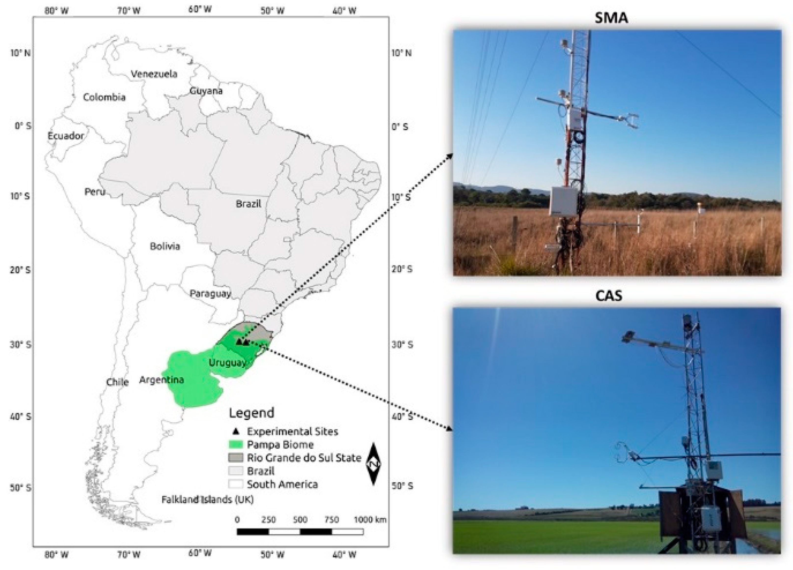
2.1. Site and Instrumentation

The data used in this study were collected in two experimental sites located in the Pampa biome in Southern Brazil that were roughly 60 km away distant from each other (Figure 1). The Santa Maria site (SMA) is located in an area of native grassland that belongs to the Federal University of Santa Maria (UFSM) in Santa Maria, Rio Grande do Sul State (29° 43′ 26.76″ S and 53° 45′ 34.92″ W, altitude of 88 m). This site is commonly used for cattle production. The Cachoeira do Sul site (CAS) is located on a flooded rice paddy field in Cachoeira do Sul, Rio Grande do Sul State (30° 16′ 37.59″ S and 53° 8′ 52.25″ W, altitude of 40.5 m). The rice is cultivated from November to April and the surface remains fallow for the rest of the year. The climate in the experimental sites is classified as subtropical humid (Cfa, Köppen climate classification; [39]), with high summer temperatures (~35 °C) and low winter temperatures, which can even reach negative temperatures and with the occurrence of frost. The precipitation for both sites is well distributed year-round (between 83 and 157 mm by month (1961–1990 according to Brazilian National Meteorological Service (INMET) [40], and the daily average of relative humidity is high throughout the year [41].

In the SMA site, the L↓ and global solar radiation (R_g) were measured by the net radiation sensor (CNR4, Kipp & Zonen, Deft, The Netherlands), while the relative humidity (RH) and air temperature (T_a) were measured using the thermo-hygrometer sensor (HMP155, Vaisala, Finland), all at the height of 3 m. The data period used in this study was from January 2014 to December 2019. More details on the SMA site are described in Zimmer et al. [42] and Rubert et al. [43].

In the CAS site, the L↓ was measured by a pyrgeometer (CG1, Kipp & Zonen, Deft, The Netherlands) and R_g by a pyranometer (LI200S, LI-COR Inc., Lincoln, NE, USA) at 6 m height and RH and T_a by a thermo-hygrometer (CS215-L, Campbell Scientific Inc., Logan, UT, USA) at 3 m height. Data were collected between 20 February 2013 and 19 February 2016. More details on the CAS site are described in Diaz et al. [44] and Souza et al. [45].

Measurements were processed in 30 min in both sites. Actual vapor pressure (e_a, hPa) was obtained according to Allen et al. [46]:

$$e_{a }\left(T_a, \mathrm{RH}\right)=\left(6.1078{\exp }^{\left[\frac{17.27{ \mathrm{T}}_{\mathrm{a}}}{{\mathrm{T}}_{\mathrm{a}} + 237.3}\right]}\right)\left(\frac{\mathrm{RH}}{100}\right)$$

(1)

where: T_a is the air temperature (°C) and RH is the relative humidity (%).

2.2. Clearness Index

The daily clearness index of the atmosphere (K_t) over shortwave wavelengths (0.3–0.7 µm) represents the atmospheric transmissivity and is defined as the ratio between the daily integrated shortwave radiation received on surface-level (measured global solar radiation, R_g) and the daily shortwave radiation coming from the sun that is theoretically received at the top of the atmosphere (R₀) (extraterrestrial solar radiation) [2].

According to Kuye and Jagtap [47], the daily clearness index is used to classify the daily sky cover as cloudy sky (CD) for K_t values between 0 and 0.35, partly cloudy sky (CP) for K_t values between 0.35 and 0.65, and clear sky (CS) for K_t values between 0.65 and 1. We adopt such classification in the present work.

2.3. Evaluated Parameterizations

The longwave radiation emitted from the atmosphere to the surface can be estimated by the Stefan–Boltzmann equation:

$$L\downarrow = {\epsilon }_e\sigma T_a{}^4$$

(2)

where: σ is the Stefan–Boltzmann constant (5.67 × 10⁻⁸ Wm⁻² K⁻⁴) and ε_e and T_a (K) are the effective emissivity and the temperature of the atmosphere. The temperature and emissivity are integrated quantities over an atmospheric column above the ground that emits longwave radiation. However, ε_e and T_a are typically estimated from ground-based meteorological observations in most models for L↓ based on Equation (2). In general, the methods to estimate the effective emissivity ε_e corresponding to the atmospheric emissivity under clear sky conditions are based on the ambient temperature and water vapor pressure (ε_CLR (T_a, e_a)) [12,13,14,15,16,17,18,20]. The clouds increase the amount of L↓ reaching the surface by changing the emissivity and temperature of the atmosphere. Therefore, the emissivity should be able to include the effects of the cloud (i.e., effects of the sky cover), and various equations have attempted to estimate the increased L↓ produced by clouds [27,35,36,37,48,49,50].

In order to obtain the effective emissivity of the atmosphere for all sky cover conditions, a general form for ε_e combines the atmospheric emissivity under clear sky conditions (ε_CLR (T_a, e_a)) with the cloud sky correction (g(K_t)). To obtain the cloud sky correction, many models of sky cover fraction have been proposed, which is also called cloud cover fraction [27,48,51,52,53,54,55]. To simplify, we suggest the cloud sky correction function using the clearness index (K_t). Thus, the effective emissivity can be written as

$${\epsilon }_e \left(T_a, e_a, K_t\right)$$

(3)

defining:

$$g\left(K_t\right)=1 + \mu {[C\left(K_t\right)]}^{\lambda }$$

(4)

where μ and λ are parameters to be adjusted (hereafter called coefficients), and C(K_t) is the sky cover fraction function (as defined in Marthews et al. [28]). The term g(K_t) in Equation (3) guarantees increased emissivity when clouds are present, representing a correction function that considers sky coverage. Equation (4) is based on the models proposed by Iziomon et al. [34], Jacobs [36], Maykut and Church [35], Sugita and Brutsaert [37] and Choi et al. [56]. Therefore, if μ is zero, Equation (3) represents the clear sky emissivity; in other cases, the influence of cloudiness will be analyzed from the joint calibration of the sky’s emissivity equations (ε_CLR (T_a, e_a)) and the sky cover correction function g(K_t).

Some equations for ε_CLR and its original coefficients are presented in

Table 1. Equations for atmospheric emissivity under clear sky conditions, ε_CLR (T_a, e_a), and original coefficients. T_a is the air temperature (K) and e_a is the water vapor pressure (hPa).

			Original Coefficients
Reference	Code	${\epsilon }_{CLR} \left(T_a, e_a\right)$	a1	a2	a3
Ångströn (1915) [58]	EAN	$a_1-a_2 {10}^{-a_3.e_a}$	0.83	0.18	0.067 [hPa−1]
Brunt (1932) [59]	EBR	$a_1+a_2 {(e_a)}^{1/2}$	0.52	0.065 [hPa−1/2]	-
Swinbank (1963) [60]	ESW	$a_1 T_a^2$	9.36 × 10−6 [K−2]	-	-
Idso and Jackson (1969) [13]	EIJ	$1-a_1 exp(-a_2\left(T_a-273.13{)}^2\right)$	0.261	0.00077 [K−2]	-
Brutsaert (1975) [14]	EBT	$a_1{\left(\raisebox{1ex}{$e_a$}\!\left/ \!\raisebox{-1ex}{$T_a$}\right.\right)}^{1/7}$	1.24[$\left(\frac{K}{hPa}\right)$1/7]	-	-
Satterlund (1979) [15]	EST	$a_1\left[1-exp\left(-{(a_2 e_a)}^{\raisebox{1ex}{$T_a$}\!\left/ \!\raisebox{-1ex}{$2016$}\right.}\right)\right]$	1.08	1.0 [hPa−1]	-
Idso (1981) [16]	EID	$a_1+a_2 \left[e_a exp\left(\raisebox{1ex}{$1500$}\!\left/ \!\raisebox{-1ex}{$T_a$}\right.\right)\right]$	0.7	5.95 × 10−5 [hPa−1]	-
Garrat (1992) [17]	EGR	$a_1+a_2 exp \left(-a_3 e_a\right)$	0.79	0.17	0.96 [hPa−1]
Konzelmann (1994) [48]	EKZ	$a_1+a_2 {\left(\raisebox{1ex}{$e_a$}\!\left/ \!\raisebox{-1ex}{$T_a$}\right.\right)}^{1/a_3}$	0.23	0.484 [K hPa−1]	8.00
Prata (1996) [61]	EPR	$1-\left(1 + w\right)exp\left[-{(a_1 + a_2 w)}^{0.5}\right]$; $w= 46.5 \left(\raisebox{1ex}{$e_a$}\!\left/ \!\raisebox{-1ex}{$T_a$}\right. \right)$	1.2	3.0 [g−1cm2]	-
Niemelä (2001) [18]	ENM	$a_1+a_2\left(e_a-2\right)$	0.72	0.009; if $e_a$ $\ge$ 2 −0.076; if $e_a$ $<$ 2 [hPa−1]	-

. It is important to note that each coefficient has different units to make atmospheric emissivity dimensionless. Equations EAN [12,18,19,57] only use e_a in their formulation, while EST [12,13] uses T_a, and EBT [7], EST [8], EID [9], EPR [30], and EKZ [48] use both meteorological variables. The EBT and EPR models are physically based models. The EBT model is based on the analytic solution of the Schwarzschild equation for the standard atmospheric lapse rates of $T_a$ and $e_a$, and the EPR model was based on radiative transfer simulations. The other models were proposed empirically by using observations of longwave radiation for definite atmospheric conditions. Both physical and empirical model parameters and performance are significantly affected by geographical location and local atmospheric conditions and require site-specific validation and parameterization [57].

Three parameterizations for estimating the sky cover fraction function C(K_t) are presented in

Table 2. Equations for sky cover fraction function C(K_t).

Reference	Code	C(Kt)
Black (1956) [51]	CQB	$(0.34 – {\left( {\left(0.34\right)}^2+4\times 0.458\times \left(0.803-K_t\right)\right)}^{0.5})/\left(-0.916\right)$
Campbell (1985) [52]	CCB	$2.33-3.33 K_t$
Wheishampel and Urban (1996) [54]	CWU	$1+\left[252.7-\left(R_g\times 60\times 60\times 24\right)/\left(4.19\times 10.000\right)\right]/$$\left[0.695 \left(R_g/K_t\right)\times 60\times 60\times 24\right)/\left(4.19\times 10.000\right)]$

and used in this work. Many schemes to estimate sky cover fraction function are present in the literature. Kasten and Czeplak [53], Crawford and Duchon et al. [27], Konzelmann et al. [48], and Jegede et al. [55] have suggested equations that depend on theoretical clear sky estimations, in which the estimation of atmosphere turbidity and pressure-correction air function are necessary (as described in Marthews et al. [28]). Here, we decided to only use parameterizations using K_t as a variable.

2.4. Proposed Model

A new empirical clear sky emissivity model for atmosphere downward longwave radiation is proposed:

$${\epsilon }_{CLR} \left(T_a, e_a\right)=a_1\left(\frac{\left(T_a-273.16\right)}{ e_a}\right) + a_2\left(\frac{e_a}{100}\right) +a_3\left(\frac{T_a}{273.16}\right)$$

(5)

where the values of a₁, a₂, and a₃ are the parameters to be adjusted. The acronym EAI is used for this proposed equation. This proposal was formulated empirically using mathematical expressions based on classical equations variables (Table 1). The Equation (5) describes a multiple regression analysis performed between the experimental [L↓/($\sigma T_a{}^4$)] and two atmospheric variables (T_a, e_a) for clear sky days. The first term of Equation (5) connects the air temperature and the water vapor pressure. Water vapor in the atmosphere varies widely for small differences in the temperature and pressure conditions. The second term is related to relative humidity, which is represented by the actual vapor pressure. The third and final term is relative to air temperature.

2.5. Statistical Indexes and Analysis

L↓ estimations were compared with experimental data using the correlation coefficient (R²), the root mean square error (RMSE), and percentage bias (PBias). These statistical indices are defined by

$$R^2=\frac{{{\displaystyle \sum }}_{i=1}^N{\left(\left(L_{exp}{\downarrow }_i- \overline{L_{exp}\downarrow }\right)\left(L{\downarrow }_i- \overline{L\downarrow }\right)\right)}^2}{{{\displaystyle \sum }}_{i=1}^N{\left(L_{exp}{\downarrow }_i- \overline{L_{exp}\downarrow }\right)}^{ 2}{{\displaystyle \sum }}_{i=1}^N{\left(L{\downarrow }_i- \overline{L\downarrow }\right)}^{ 2}}$$

(6)

$$RMSE={\left(\frac{1}{\mathrm{N}}{\displaystyle \sum }_{\mathrm{i}=1}^{\mathrm{N}}{\left(L{\downarrow }_i-L_{\exp }{\downarrow }_i\right)}^2\right)}^{1/2}$$

(7)

$$PBias=\frac{{{\displaystyle \sum }}_{i=1}^{\mathrm{N}}\left(L{\downarrow }_i-L_{\exp }{\downarrow }_i\right)}{{{\displaystyle \sum }}_{i=1}^{\mathrm{N}}\left(L_{\exp }{\downarrow }_i\right)}\times 100$$

(8)

where i is the sampler, L↓ is the simulated atmospheric downward longwave radiation, L_exp↓ is the experimental atmospheric downward longwave radiation, ($\overline{L\downarrow }$) is the average of the simulated values, ($\overline{L_{\exp }\downarrow }$) is the average of experimental values, and N is the number of simulated data. The analysis of the correlation coefficient results follows the classification suggested by Cohen [62].

Half-hour experimental atmospheric downward longwave radiation measurements obtained at the SMA site for the entire year of 2014 were used to evaluate the models. The sequence of analyses was:

Step 1—evaluation of Equation (2) using Equations (3) and (4) with μ = 0 and ε_CLR (T_a, e_a) from Table 1 and original coefficients;

Step 2—calibration of Equation (2) using Equations (3) and (4) with μ = 0 and ε_CLR (T_a, e_a) from Table 1 and the new proposed equation (Equation (5));

Step 3—calibration of Equation (2) using Equations (3) and (4) with μ ≠ 0, C(K_t) from Table 2, ε_CLR (T_a, e_a) from Table 1, and the new proposed equation (EAI—Equation (5));

Step 4—validation of Equation (2) using the best results from Step 2 and 3 for both experimental sites.

Because K_t cannot be calculated during the night, the C(K_t) was determined using the daily K_t (or daily average). Therefore, in Steps 3 and 4, we used the equations of ε_CLR for half-hour measurements combined with one value for C(K_t) for the entire day. The analyses were performed for different daily sky cover classifications, as described in Section 2.2.

The combination of Equations (3) and (4) yielded 48 possible solutions for Equation (2). In the coefficient calibration process, each one of them was adjusted by the non-linear least squares method. We used the MATLAB (Mathworks Inc.) program and lsqcurvefit function from Optimization Toolbox™ to solve the least squares method. Only SMA site data from 2014 were considered in the calibration algorithm and individual analysis for each class of sky cover performed. The performance of the models’ combination was evaluated using the best RMSE (near zero).

3. Results and Discussion

3.1. Evaluation of L↓ Models for SMA Site for 2014

The SMA experimental data for 2014 used to evaluate the L↓ equations presents the following sky cover classification: 27.40% for clear sky days (CS), 46.57% for partly cloudy days (CP), and 21.64% for cloudy days (CD). The clearness index did not show seasonality for SMA (data not shown).

3.1.1. Using Original Coefficients—Step 1

The atmospheric downward longwave radiation estimates were obtained by following Step 1. The statistical results of the eleven equations used to estimate L↓ are shown in

Table 3. Statistical index for the entire period and for different sky coverage classifications for Step 1. The best results are colored in green and the worst in red.

	Entire Period			CS			CP			CD
${\mathit{\epsilon }}_{\mathit{CLR}} ({\mathit{T}}_{\mathit{a}}, {\mathit{e}}_{\mathit{a}})$	R2	RMSE (Wm−2)	PBias (%)	R2	RMSE (Wm−2)	PBias (%)	R2	RMSE (Wm−2)	PBias (%)	R2	RMSE (Wm−2)	PBias (%)
EAN	0.59	44.79	−9.71	0.73	29.54	−5.23	0.62	45.26	−10.21	0.59	59.78	−14.50
EBR	0.67	50.42	−11.49	0.78	38.590	−8.53	0.68	49.60	−11.17	0.65	64.69	−15.70
EGR	0.54	55.10	−12.67	0.69	36.54	−7.77	0.59	56.64	−13.43	0.54	72.03	−17.61
ENM	0.67	30.92	−3.47	0.78	26.61	−0.32	0.68	30.06	−3.03	0.64	37.55	−8.13
ESW	0.53	51.65	−10.85	0.69	37.17	−6.07	0.59	51.10	−11.06	0.53	68.12	−16.48
EIJ	0.53	49.93	−10.20	0.67	35.47	−5.26	0.59	49.27	−10.41	0.52	66.44	−16.01
EBT	0.66	38.57	−7.75	0.77	28.24	−4.36	0.67	37.72	−7.65	0.65	50.98	−12.16
EST	0.61	35.87	−6.57	0.74	24.77	−2.15	0.64	35.14	−6.90	0.60	48.66	−11.56
EID	0.70	25.48	−2.18	0.79	22.91	0.87	0.69	24.56	−1.97	0.66	30.30	−6.34
EPR	0.65	38.87	−7.89	0.77	27.51	−4.25	0.67	38.19	−7.90	0.64	51.88	−12.42
EKZ	0.62	141.64	−36.75	0.75	122.68	−33.84	0.66	144.85	−36.97	0.61	160.07	−40.03

. For entire period (EP) and all sky classifications, the EID presented the best results in all analyzed statistical indexes. The ESW and EIJ equations presented the worst results for R² in all periods, while the EKZ showed the worst results for RMSE and PBias. All equations presented better R² for CS with values above 0.67. This was expected because the original equations were developed for clear sky conditions. In general, all results showed the considered models to underestimate L↓ (negative PBias) with errors above 20 Wm⁻². The errors increased as the clearness index decreased. According to Marthews et al. [28], the analysis of L↓ over a tropical lowland forest revealed that RMSE values below or equal to 20 Wm⁻² are acceptable for L↓ estimates.

Generally, both physical and empirical model parameters and performance are significantly affected by geographical location and local atmospheric conditions and require site specific validation and parameterization [56]. Therefore, all L↓ equations of Table 1 need to be calibrated for the Brazilian Pampa regions to increase the accuracy of the models, as also highlighted by Li et al. [29].

3.1.2. Calibrating the Coefficients—Step 2

We calibrated the coefficients (a₁, a₂, a₃) of the L↓ according to Step 2. The new proposed equation (L↓ EAI) was also calibrated. The results of the models’ performances are presented in

Table 4. Calibrated coefficients and statistical index for the entire period and different sky coverage classifications for Step 2. The best results are colored in green and the worst in red. RMSE in (Wm⁻²) and PBias in (%).

${\mathit{\epsilon }}_{\mathit{CLR}} ({\mathit{T}}_{\mathit{a}}, {\mathit{e}}_{\mathit{a}})$	Entire Period				CS				CP				CD
	${\mathit{a}}_1$$/{\mathit{a}}_2$$/{\mathit{a}}_3$	R2	RMSE	PBias	${\mathit{a}}_1$$/{\mathit{a}}_2$$/{\mathit{a}}_3$	R2	RMSE	PBias	${\mathit{a}}_1$$/{\mathit{a}}_2$$/{\mathit{a}}_3$	R2	RMSE	PBias	${\mathit{a}}_1$$/{\mathit{a}}_2$$/{\mathit{a}}_3$	R2	RMSE	PBias
EAN	0.94/0.21/0.04	0.61	26.03	0.15	5.34/4.52/2.22 × 10−4	0.73	23.21	0.23	0.94/0.06/0.02	0.61	22.90	0.06	0.97/1.14/0.13	0.61	16.05	0.03
EBR	0.77/0.03/-	0.61	26.13	0.15	0.78/0.02/-	0.73	23.26	0.21	0.87/0.01/-	0.61	22.90	0.06	0.87/0.02/-	0.59	16.49	0.03
ESW	1.05 × 10−5/--/-	0.53	34.25	0.13	9.99 × 10−6/-/-	0.69	32.69	0.31	1.05 × 10−5/-/-	0.59	31.34	0.08	1.12 × 10−5/-/-	0.53	21.18	0.03
EIJ	0.08/−3.76 × 10−4/-	0.54	26.81	−0.07	0.14/−1.22 × 10−4/-	0.68	24.05	0.02	0.07/−5.0 × 10−4/-	0.59	22.37	−0.07	0.02/−1.3 × 10−3/-	0.55	16.40	−0.03
EBT	1.35/-/-	0.66	26.60	0.19	1.30/-/-	0.77	24.92	0.33	1.34/-/-	0.67	25.29	0.11	1.41/-/-	0.65	17.92	0.05
EST	2.94/5.57 × 10−5/-	0.67	23.55	−0.06	2.96/3.75 × 10−5/-	0.77	20.91	−0.22	0.91/1.47 × 107/-	0.59	23.02	0.02	4.49/2.72 × 10−6/-	0.66	14.72	−0.05
EID	0.77/4.54 × 10−5/-	0.67	24.24	0.16	0.76/3.40 × 10−5/-	0.76	21.88	0.24	0.83/2.46 × 10−5/-	0.65	22.13	0.08	0.87/2.59 × 10−5/-	0.62	15.96	0.04
EGR	0.90/7.43/7.91	0.54	27.25	0.01	0.86/−4.91/10.57	0.69	24.06	0.09	0.91/8.16/7.06	0.59	23.02	0.02	0.96/8.30/6.87	0.54	16.84	−0.09
EKZ	0.90/−5.15/0.12	0.54	27.25	0.01	0.86/−5.76/0.07	0.69	24.06	0.09	0.86/0.24/1.82	0.62	22.83	0.06	0.96/−4.86/0.06	0.54	16.84	−0.01
EPR	2.07/4.08/-	0.63	25.82	0.18	3.65/2.59/-	0.73	23.02	0.20	5.97/2.83/-	0.62	22.83	0.07	−0.58/7.23/-	0.62	16.24	0.13
ENM	0.84/3.60 × 10−3/-	0.61	26.20	0.14	0.82/2.5 × 10−3/-	0.73	23.18	0.22	0.89/1.2 x10−3/-	0.61	22.90	0.06	0.92/2.1 × 10−3/-	0.58	16.55	0.02
EAI	−0.20/−0.07/1.05	0.72	21.16	−0.03	−0.15/−0.07/0.98	0.82	18.18	−0.02	−0.22/−0.29/1.12	0.71	18.72	−0.05	−0.22/−0.40/1.18	0.67	14.06	−0.02

with the respective calibrated parameter values. The calibrated coefficient values are small for some parameters and even large for the same parameterization in others, as also noted by Carmona et al. [19] and Zhu et al. [63]. By comparing the statistical indices of the models from Table 2 and Table 3, the PBias was reduced drastically by the calibration (around two order of magnitude) in all sky cover classification, resulting in the overestimation for most of them. In general, RMSE was reduced for all sky cover classifications, from 1% for EID to 85% for EKZ. Nevertheless, the analysis of the different sky cover classifications shows that the RMSE decreased by around 40% when the clearness index decreased, in addition to R² slightly decreasing. These results are likely due to the small variability of the downward longwave radiation in experimental data, as shown in the x axis of Figure 1 when the clearness index decreased.

In general, the EST presented the smallest errors of the classic calibrated models, with a slight underestimation of the experimental data (negative Pbias), followed by an EID model with errors around 3% higher, although with overestimation (positive Pbias). The worst results were found for ESW, with errors greater than 30 Wm⁻² except for CD sky cover classification (21.18 Wm⁻²).

Guo et al. [64] evaluated six models (which were also evaluated in this study: EBR, ESW, EIJ, EBT, EID, EPR) for 71 globally distributed sites and reported that the worst results were obtained by equations that did not consider e_a in their parametrization (ESW and EIJ). Similar results were found by Carmona et al. [19], who evaluated the same models for a site in the sub-humid Pampean region in Argentina. Here, after calibration, ESW also had the worst results, followed by EKZ and EGR, which, however, are functions of e_a (EKZ is also a function of T_a).

The dispersion between the experimental and estimated EAI L↓ are shown in Figure 2. The EAI overestimated the lowest experimental L↓ values, especially during night periods (Figure 3). Principally in CD conditions, the high experimental L↓ values are better represented by EAI. In general, the EAI presented a better performance for all sky cover classifications compared to the classical equations (Table 4). Moreover, this equation showed the smallest variability in the statistical index for different sky cover classifications, indicating that this formulation accurately represents all sky conditions even using the EP calibration. The best performance of the EAI can be due to the equation was obtained over periods of entire days classified as clear sky. On these days, the sky may have presented some moments of lower clearness indices (some clouds in the sky), but that can be masked by the daily average sky cover classification.

3.1.3. Calibrating the Coefficients—Step 3

We calibrated the coefficients (a₁, a₂, a₃, λ, μ) of the L↓ obtained from Equations (2) and (3) with the ε_CLR (T_a, e_a) from (Table 1) and C(K_t) from (Table 2). The results of the five best combinations for each sky cover classification are presented in

Table 5. Calibrated coefficients and the statistical index for the entire period and different sky coverage classifications for the five best results in Step 3.

${\mathit{\epsilon }}_{\mathit{C}\mathit{L}\mathit{R}}\left({\mathit{T}}_{\mathit{a}}, {\mathit{e}}_{\mathit{a}}\right)\_\mathit{C}\left({\mathit{K}}_{\mathit{t}}\right)$	a1	a2	a3	μ	λ	R2	RMSE (Wm−2)	Pbias (%)
Entire Period
EST_CQB	5.45	2.76 × 10−7	-	0.13	0.95	0.78	17.82	−0.06
EBT_CQB	1.27	-	-	0.14	1.44	0.76	22.40	−0.39
EID_CQB	0.76	2.71 × 10−5	-	0.15	1.10	0.75	19.73	−0.16
EST_CCB	4.96	2.29 × 10−7	-	0.07	0.56	0.73	17.52	−0.14
EKZ_CQB	0.68	0.32	3.85	0.17	1.01	0.73	20.48	−0.17
CS
EST_CCB	4.81	8.46 × 10−7	-	0.27	1.19	0.80	18.06	−0.07
EST_CQB	3.80	4.44 × 10−6	-	0.14	1.12	0.79	19.28	−0.09
EBT_CCB	1.29	-	-	443.41	84.01	0.79	23.42	−0.52
EID_CCB	0.76	3.42 × 10−5	-	28.53	3.51	0.79	19.46	−0.20
EBT_CQB	1.18	-	-	0.11	0.09	0.79	23.20	−0.47
CP
EST_CQB	3.19	1.42 × 10−7	-	1.10	0.13	0.72	18.52	−0.07
EST_CCB	3.55	8.23 × 10−6	-	0.08	0.72	0.71	19.49	−0.17
EBT_CQB	1.29	-	-	0.21	2.49	0.71	23.76	−0.42
EBT_CCB	1.30	-	-	0.06	1.42	0.71	23.76	−0.42
EID_CCB	0.80	2.36 × 10−5	-	0.06	1.15	0.69	20.71	−0.17
CD
EST_CWU	0.94	8.18 × 10−8	-	0.52	0.49	0.68	14.00	−0.17
EST_CQB	1.92	8.71 × 10−6	-	1.06	0.20	0.68	14.58	−0.08
EBT_CQB	2.58	-	-	−0.44	−0.15	0.67	17.31	−0.19
EBT_CCB	1.39	-	-	0.00	4.36	0.67	17.27	−0.18
EST_CCB	1.97	1.69 × 10−4	-	0.32	0.28	0.67	15.25	−0.12

with the respective calibrated parameter values. By adding a cloud sky correction, all combinations presented better results than without this correction for all sky cover classifications, where, in general, RMSE decreased by around 5 Wm⁻² and R² increased by almost 10%. The EST and EID models are present in all five of the best results, especially CQB and CCB sky cover fraction functions. The smallest errors were obtained in CD classification, where EST_CWU presented the best result, although the R² was lower in this sky classification. For the other sky cover classifications, in general, the best results were obtained by EST_CCB and EST_CQB.

The results of all combinations using the new proposed equation (EAI) are presented in

Table 6. Calibrated coefficients and statistical index for the entire period and different sky coverage classifications for EAI in Step 3.

${\mathit{\epsilon }}_{\mathit{C}\mathit{L}\mathit{R}}\left({\mathit{T}}_{\mathit{a}}, {\mathit{e}}_{\mathit{a}}\right)\_\mathit{C}\left({\mathit{K}}_{\mathit{t}}\right)$	a1	a2	a3	μ	λ	R2	RMSE (Wm−2)	PBias (%)
Entire Period
EAI_CQB	−0.17	−0.25	1.01	0.13	1.12	0.79	17.23	−0.01
EAI_CCB	−0.19	−0.31	1.06	0.06	0.71	0.75	16.63	0.00
EAI_CWU	−0.02	−0.01	0.09	0.04	1.01	0.72	20.80	−0.02
CS
EAI_CCB	−0.16	−0.22	1.02	1.75	2.35	0.83	16.46	0.00
EAI_CWU	−0.01	−0.01	0.07	0.09	0.90	0.82	18.01	−0.01
EAI_CQB	−0.14	−0.12	0.97	1.47	3.39	0.82	17.89	−0.04
CP
EAI_CCB	−0.20	−0.30	1.04	0.09	0.47	0.74	17.68	0.00
EAI_CQB	−0.19	−0.28	0.97	0.21	0.55	0.74	17.69	0.00
EAI_CWU	−0.02	−0.03	0.10	0.03	1.05	0.71	18.57	−0.01
CD
EAI_CCB	−0.21	−0.38	1.14	0.01	2.44	0.69	13.82	0.00
EAI_CQB	−0.21	−0.38	1.14	0.04	4.54	0.69	13.82	0.00
EAI_CWU	−0.19	−0.36	1.02	0.27	−0.11	0.68	14.10	0.00

. The EAI equation with sky cover fraction function combinations had better performance than the results demonstrated before, with an RMSE below 20 Wm⁻² in all sky cover classifications. The RMSE decreased by no more than 20% from the calibrated one without C(K_t) (comparing Table 4 with Table 6). For CD, there was no significant difference (<3%) in the results with C(K_t). As the EAI was formulated considering the daily mean of K_t, when implementing the parameterization of cloud cover C(K_t), no significant influence was observed.

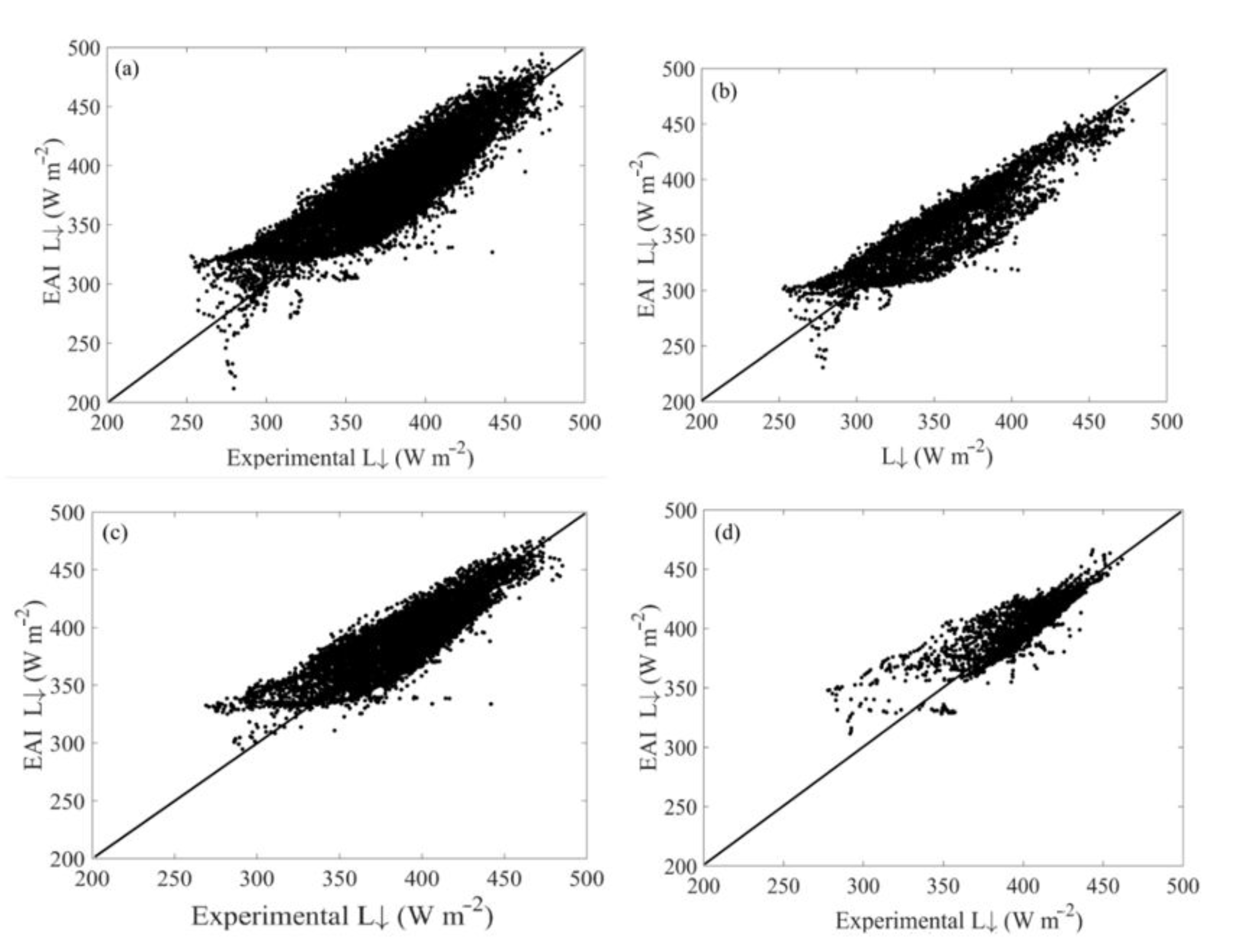
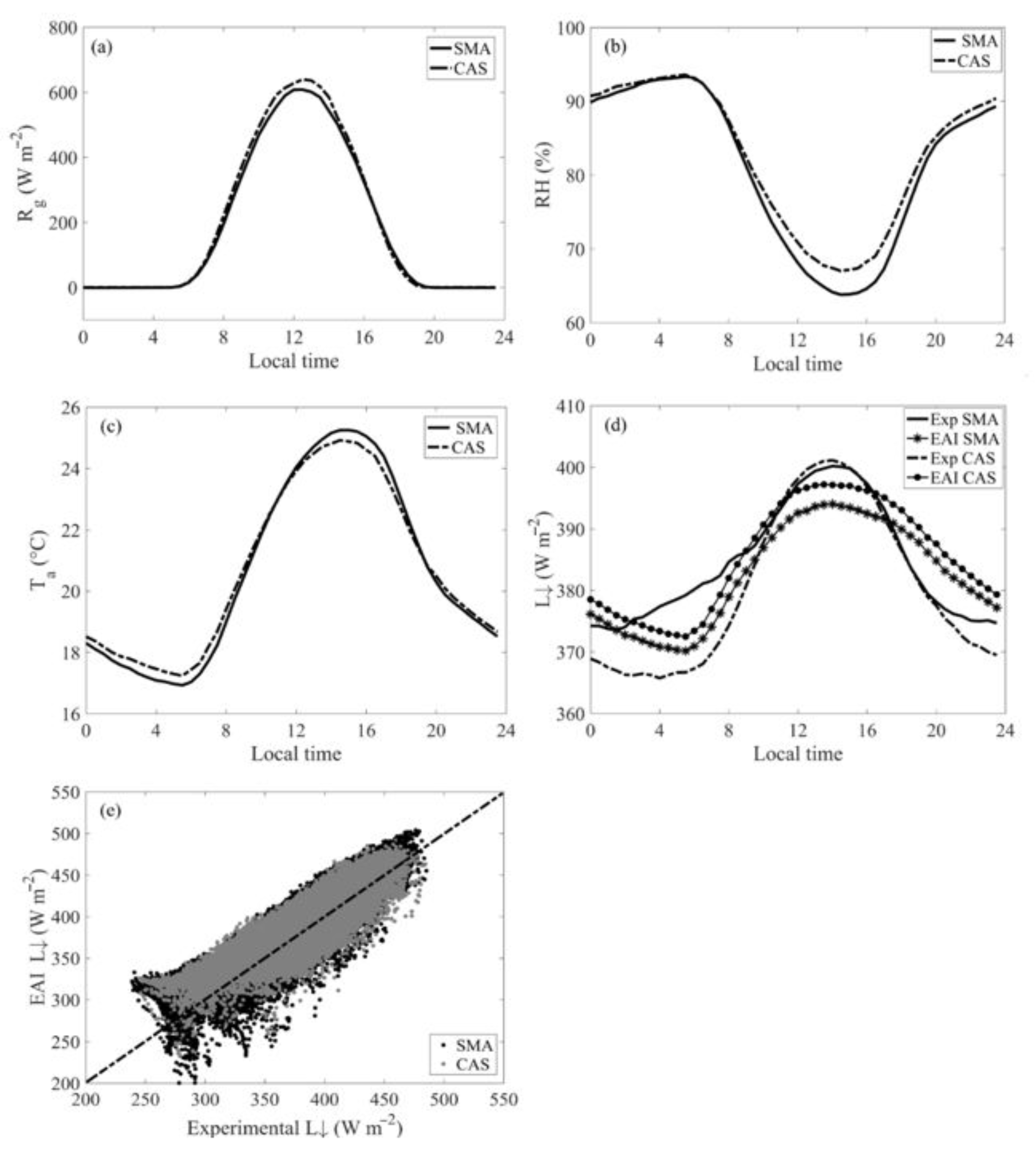
3.1.4. Validation of a New Proposed Downward Longwave Radiation—Step 4

In general, EAI presented better results than the classical equations for all sky covers (CS, CP, CD) and did not significantly improve the results using the cloud sky correction, indicating that the EAI is recommended to use in this region, even without considering the cloud sky correction. Here, we will evaluate the EAI calibrated over the entire period (Table 6).

To evaluate whether the L↓ (EAI) equation obtained by calibration for SMA adequately describes the downward longwave radiation at different locations in the Pampa biome, we used data from the SMA (the entire years of 2015–2019) and CAS (from 20 February 2013 to 16 April 2016) experimental sites. To compare EAI with a classical model, we will also present EST results, which is a model that showed the best results in all evaluations (Table 5).

The EAI equation applied to CAS presented similar results to SMA for R² and PBias (~1%) and a difference of around 10% regarding the RMSE (

Table 7. Mean L↓ estimated by the EAI and EST equations using coefficients for the entire period. Experimental L↓ was 375.69 Wm⁻² for Santa Maria experimental site (SMA) and 374.89 Wm⁻² for Cachoeira do Sul experimental site (CAS); ESTorig uses the original coefficients from Table 1 and ESTcal uses the calibrate coefficients from Table 4. Equations were combined with the cloud sky correction function using parameters from Table 5.

${\mathit{\epsilon }}_{\mathit{C}\mathit{L}\mathit{R}}\left({\mathit{T}}_{\mathit{a}}, {\mathit{e}}_{\mathit{a}}\right)\_\mathit{C}\left({\mathit{K}}_{\mathit{t}}\right)$	L↓ (Wm−2)	RMSE (Wm−2)	R2	PBias (%)
SMA (1 January 2015 to 31 December 2019)
EAI	381.49	22.84	0.69	1.54
EAI_CQB	383.45	18.59	0.79	1.44
EAI_CCB	389.96	18.37	0.76	1.46
EAI_CWU	381.34	22.75	0.70	1.50
ESTorig	354.55	33.71	0.60	−5.62
ESTcal	407.53	40.65	0.66	8.47
EST_CQB	383.11	18.52	0.78	1.35
EST_CCB	340.09	47.58	0.75	−11.51
EST_CWU	381.53	22.57	0.70	1.55
CAS (20 February 2013 to 16 April 2016)
EAI	379.88	25.33	0.67	1.33
EAI_CQB	388.00	20.47	0.76	1.07
EAI_CCB	392.65	20.75	0.72	1.01
EAI_CWU	388.06	25.04	0.70	1.91
ESTorig	361.33	32.60	0.61	−5.10
ESTcal	415.34	42.50	0.66	9.08
EST_CQB	387.80	20.19	0.76	1.02
EST_CCB	342.82	50.44	0.71	−11.80
EST_CWU	387.60	25.03	0.69	1.79

), showing that the proposed equation efficiently estimates L↓ in the Pampa biome. It is also noted that when we implemented the parameters for cloud sky correction in EAI, the results improved by 20%; the same behavior was found for CAS. When comparing EAI with EST and its original coefficients without the cloud sky correction, the EAI presented the best results. After incorporating the parameterizations in EST, the statistical indices significantly improved except for using CCB. Nevertheless, using the CQB and CWU parameterizations presented the same statistical indices in both sites for both EAI and EST.

The SMA and CAS experimental sites are approximately 60 km far from each other, although they have a significantly different land cover. The SMA surface is covered with natural grassland used by cattle, while CAS is in a lowland rice paddy. However, comparing the diurnal cycle of atmospheric variables for the same data period for the SMA and CAS sites, we can see very similar behavior from 1 January 2014 to 16 April 2016 (Figure 3). The most notable difference is in diurnal RH when SMA presents smaller values than CAS. The experimental L↓ in CAS and SMA are quite similar during the day, but in the night period, SMA is around 10 Wm⁻² greater than CAS (primarily in the night and early morning, from 0 to 8 h).

The new model presented proved to be valid, given the results reported herein, in which EAI fit well without requiring specific calibration for CAS. Therefore, the EAI equation can be an excellent alternative to represent L↓ regarding similar weather conditions. Thus, the proposed equation (EAI) presented a good performance to estimate L↓ in the Brazilian Pampa biome with values similar to those obtained by Carmona et al. [19], who developed a model for a region with similar vegetation to that analyzed here (Argentinian Pampa) but included a sky cover fraction (cloud fraction) in their formulation for L↓. In Carmona et al. [19], two equations are proposed, one only for clear sky and another for all sky conditions. However, they used the RH as atmospheric variables in emissivity equations, and to calculate the sky cover fraction, it is necessary to estimate the theoretical solar radiation received in clear-sky conditions, depending on the sky conditions such as the turbidity coefficient and atmospheric pressure. Nonetheless, here we chose to analyze only equations using e_a and/or T_a, and we suggest employing equations for a sky cover fraction that only needs the clearness index calculated using the extraterrestrial solar radiation, making the proposed approach much easier to estimate L↓.

4. Conclusions

An L↓ estimation analysis using different equations for emissivity and cloud sky correction concerning experimental data measured in the SMA site was presented. First, eleven well known L↓ models were analyzed for SMA to test their accuracy under different sky cover classifications (CS, CP, and CD). The results showed that all models presented high error and underestimated values compared to the experimental data. Thus, it was necessary to calibrate the equation’s coefficients to adjust the L↓ models, leading to better statistical indexes.

A general structure to the cloud sky correction was added to the clear sky emissivity models to improve L↓ estimates and determine how they influence cloud presence in the different periods analyzed. Moreover, we did a joint calibration between the clear sky emissivity model and cloud sky correction. The results showed a considerable improvement in the RMSE compared to the models without cloud sky correction function, especially under CD conditions. However, one limitation of this study was calculated for C(Kt) in the daily mean.

A new equation (EAI) was developed to reproduce L↓ data more accurately. The EAI was calibrated for SMA and showed better performance than the other models tested, with an RMSE ranging from 13 to 21 Wm⁻², PBias close to zero, and higher values than the correlation coefficient.

The EAI equation was evaluated for a long-term dataset for SMA and CAS with good results. The model proposed has a simple parameterization using the fundamental meteorological variables water vapor pressure and air temperature, and its formulation does not require cloud sky correction to satisfactorily represent the L↓. Therefore, we recommend using the proposed equation to calculate L↓ over the Pampa biome under these specific climatic conditions and without sky cover distinction.

As a complementary part of this work, the results can be used in the verification and calibration of the Brazilian Global Atmospheric Model—BAM [65], the atmospheric component of the Brazilian Earth System Model (BESM), since most of the BAM evaluation studies have been carried out for the most tropical portion of Brazil [66], with no work using the Pampa region from southern Brazil.

References

1. Kiehl, J.T.; Trenberth, K.E. Earth’s Annual Global Mean Energy Budget. Bull. Am. Meteorol. Soc. 1997, 78, 197–208. [Google Scholar] [CrossRef] [Green Version]
2. Liou, K.-N. An Introduction to Atmospheric Radiation, 2nd ed.; Elsevier: Amsterdam, The Netherlands, 2002. [Google Scholar]
3. Garratt, J.R. Clear-Sky Longwave Irradiance at the Earth’s Surface—Evaluation of Climate Models. J. Clim. 2001, 14, 1647–1670. [Google Scholar] [CrossRef]
4. Feng, C.; Zhang, X.; Wei, Y.; Zhang, W.; Hou, N.; Xu, J.; Jia, K.; Yao, Y.; Xie, X.; Jiang, B.; et al. Estimating Surface Downward Longwave Radiation Using Machine Learning Methods. Atmosphere 2020, 11, 1147. [Google Scholar] [CrossRef]
5. Yang, F.; Cheng, J. A framework for estimating cloudy sky surface downward longwave radiation from the derived active and passive cloud property parameters. Remote Sens. Environ. 2020, 248, 111972. [Google Scholar] [CrossRef]
6. Chen, J.; He, T.; Jiang, B.; Liang, S. Estimation of all-sky all-wave daily net radiation at high latitudes from MODIS data. Remote Sens. Environ. 2020, 245, 111842. [Google Scholar] [CrossRef]
7. Cheng, J.; Liang, S. Global Estimates for High-Spatial-Resolution Clear-Sky Land Surface Upwelling Longwave Radiation From MODIS Data. IEEE Trans. Geosci. Remote Sens. 2016, 54, 4115–4129. [Google Scholar] [CrossRef]
8. Wang, K.; Dickinson, R.E. Global atmospheric downward longwave radiation at the surface from ground-based observations, satellite retrievals, and reanalyses. Rev. Geophys. 2013, 51, 150–185. [Google Scholar] [CrossRef]
9. Wang, T.; Yan, G.; Chen, L. Consistent retrieval methods to estimate land surface shortwave and longwave radiative flux components under clear-sky conditions. Remote Sens. Environ. 2012, 124, 61–71. [Google Scholar] [CrossRef]
10. Emde, C.; Buras-Schnell, R.; Kylling, A.; Mayer, B.; Gasteiger, J.; Hamann, U.; Kylling, J.; Richter, B.; Pause, C.; Dowling, T.; et al. The libRadtran software package for radiative transfer calculations (version 2.0.1). Geosci. Model Dev. 2016, 9, 1647–1672. [Google Scholar] [CrossRef] [Green Version]
11. Berk, A.; Conforti, P.; Kennett, R.; Perkins, T.; Hawes, F.; van den Bosch, J. MODTRAN6: A Major Upgrade of the MODTRAN Radiative Transfer Code. In Proceedings of the 2014 6th Workshop on Hyperspectral Image and Signal Processing: Evolution in Remote Sensing (WHISPERS), Lausanne, Switzerland, 24–27 June 2014; p. 90880H. [Google Scholar]
12. Swinbank, W.C. Long-wave radiation from clear skies. Q. J. R. Meteorol. Soc. 1963, 89, 339–348. [Google Scholar] [CrossRef]
13. Idso, S.B.; Jackson, R. D Thermal Radiation From the Atmosphere. J Geophys Res 1969, 74, 5397–5403. [Google Scholar] [CrossRef]
14. Brutsaert, W. On a derivable formula for long-wave radiation from clear skies. Water Resour. Res. 1975, 11, 742–744. [Google Scholar] [CrossRef]
15. Satterlund, D.R. An improved equation for estimating long-wave radiation from the atmosphere. Water Resour. Res. 1979, 15, 1649–1650. [Google Scholar] [CrossRef]
16. Idso, S.B. A set of equations for full spectrum and 8- to 14-μm and 10.5- to 12.5-μm thermal radiation from cloudless skies. Water Resour. Res. 1981, 17, 295–304. [Google Scholar] [CrossRef]
17. Garrat, J. The Atmospheric Boundary Layer (Cambridge Atmospheric and Space Science Series); Cambridge University Press: Cambridge, UK, 1992. [Google Scholar]
18. Niemelä, S.; Räisänen, P.; Savijärvi, H. Comparison of surface radiative flux parameterizations part I: Longwave radiation. Atmos. Res. 2001, 58, 1–18. [Google Scholar] [CrossRef]
19. Carmona, F.; Rivas, R.; Caselles, V. Estimation of daytime downward longwave radiation under clear and cloudy skies conditions over a sub-humid region. Theor. Appl. Climatol. 2014, 115, 281–295. [Google Scholar] [CrossRef]
20. Chang, K.; Zhang, Q. Modeling of downward longwave radiation and radiative cooling potential in China. J. Renew. Sustain. Energy 2019, 11, 066501. [Google Scholar] [CrossRef]
21. Liu, M.; Zheng, X.; Zhang, J.; Xia, X. A revisiting of the parametrization of downward longwave radiation in summer over the Tibetan Plateau based on high-temporal-resolution measurements. Atmos. Chem. Phys. 2020, 20, 4415–4426. [Google Scholar] [CrossRef] [Green Version]
22. Duarte, H.F.; Dias, N.L.; Maggiotto, S.R. Assessing daytime downward longwave radiation estimates for clear and cloudy skies in Southern Brazil. Agric. For. Meteorol. 2006, 139, 171–181. [Google Scholar] [CrossRef]
23. Held, I.M.; Soden, B.J. WATER VAPOR FEEDBACK AND GLOBAL WARMING. Annu. Rev. Energy Environ. 2000, 25, 441–475. [Google Scholar] [CrossRef] [Green Version]
24. Vall, S.; Castell, A. Radiative cooling as low-grade energy source: A literature review. Renew. Sustain. Energy Rev. 2017, 77, 803–820. [Google Scholar] [CrossRef] [Green Version]
25. Stephens, G.L.; Wild, M.; Stackhouse, P.W.; L’Ecuyer, T.; Kato, S.; Henderson, D.S. The Global Character of the Flux of Downward Longwave Radiation. J. Clim. 2012, 25, 2329–2340. [Google Scholar] [CrossRef] [Green Version]
26. Flerchinger, G.N.; Xaio, W.; Marks, D.; Sauer, T.J.; Yu, Q. Comparison of algorithms for incoming atmospheric long-wave radiation. Water Resour. Res. 2009, 45, 1–13. [Google Scholar] [CrossRef] [Green Version]
27. Crawford, T.M.; Duchon, C.E. An improved parameterization for estimating effective atmospheric emissivity for use in calculating daytime downwelling longwave radiation. J. Appl. Meteorol. 1999, 38, 474–480. [Google Scholar] [CrossRef]
28. Marthews, T.R.; Malhi, Y.; Iwata, H. Calculating downward longwave radiation under clear and cloudy conditions over a tropical lowland forest site: An evaluation of model schemes for hourly data. Theor. Appl. Climatol. 2012, 107, 461–477. [Google Scholar] [CrossRef]
29. Li, M.; Jiang, Y.; Coimbra, C.F.M. On the determination of atmospheric longwave irradiance under all-sky conditions. Sol. Energy 2017, 144, 40–48. [Google Scholar] [CrossRef]
30. Monteith, J.L. An empirical method for estimating long-wave radiation exchanges in the British Isles. Q. J. R. Meteorol. Soc. 1961, 87, 171–179. [Google Scholar] [CrossRef]
31. Berger, X.; Buriot, D.; Garnier, F. About the equivalent radiative temperature for clear skies. Sol. Energy 1984, 32, 725–733. [Google Scholar] [CrossRef]
32. Martin, M.; Berdahl, P. Characteristics of infrared sky radiation in the United States. Sol. Energy 1984, 33, 321–336. [Google Scholar] [CrossRef] [Green Version]
33. Heitor, A.; Biga, A.J.; Rosa, R. Thermal radiation components of the energy balance at the ground. Agric. For. Meteorol. 1991, 54, 29–48. [Google Scholar] [CrossRef]
34. Iziomon, M.G.; Mayer, H.; Matzarakis, A. Downward atmospheric longwave irradiance under clear and cloudy skies: Measurement and parameterization. J. Atmos. Solar-Terrestrial Phys. 2003, 65, 1107–1116. [Google Scholar] [CrossRef]
35. Maykut, G.A.; Church, P.E. Radiation Climate of Barrow, Alaska, 1962–66. J. Appl. Meteorol. 1973, 12, 620–628. [Google Scholar] [CrossRef] [Green Version]
36. Jacobs, J.D. Radiation climate of Broughton Island. In Energy Budget Studies in Relation to Fast-ice Breakup Processes in Davis Strait; Barry, R.G., Jacobs, J.D., Eds.; University of Colorado: Denver, CO, USA, 1978; pp. 105–120. [Google Scholar]
37. Sugita, M.; Brutsaert, W. Cloud effect in the estimation of instantaneous downward longwave radiation. Water Resour. Res. 1993, 29, 599–605. [Google Scholar] [CrossRef]
38. Boldrini, I.; Overbeck, G.; Trevisan, R. Biodiversidade de plantas. In Os Campos do Sul; UFRGS: Porto Alegre, Brazil, 2015; pp. 53–70. ISBN 978-85-66106-50-3. [Google Scholar]
39. Peel, M.C.; Finlayson, B.L.; McMahon, T.A. Updated world map of the Köppen-Geiger climate classification. Hydrol. Earth Syst. Sci. 2007, 11, 1633–1644. [Google Scholar] [CrossRef] [Green Version]
40. INMET. Instituto Nacional de Meteorologia. Available online: http://www.inmet.gov.br/portal/index.php?r=clima/normaisClimatologicas (accessed on 23 October 2020). (In Portuguese)
41. Grimm, A.M. How do La Niña events disturb the summer monsoon system in Brazil? Clim. Dyn. 2004, 22, 123–138. [Google Scholar] [CrossRef]
42. Zimmer, T.; Buligon, L.; de Arruda Souza, V.; Romio, L.C.; Roberti, D.R. Influence of clearness index and soil moisture in the soil thermal dynamic in natural pasture in the Brazilian Pampa biome. Geoderma 2020, 378, 114582. [Google Scholar] [CrossRef]
43. Rubert, G.C.; Roberti, D.R.; Pereira, L.S.; Quadros, F.L.F.; Campos Velho, H.F.D.; Leal de Moraes, O.L. Evapotranspiration of the Brazilian Pampa biome: Seasonality and influential factors. Water 2018, 10, 1864. [Google Scholar] [CrossRef] [Green Version]
44. Diaz, M.B.; Roberti, D.R.; Carneiro, J.V.; de Arruda Souza, V.; de Moraes, O.L.L. Dynamics of the superficial fluxes over a flooded rice paddy in southern Brazil. Agric. For. Meteorol. 2019, 276–277, 107650. [Google Scholar] [CrossRef]
45. Souza, V.A.; Roberti, D.R.; Ruhoff, A.L.; Zimmer, T.; Adamatti, D.S.; de Gonçalves, L.G.G.; Diaz, M.B.; Alves, R.d.C.M.; de Moraes, O.L.L. Evaluation of MOD16 algorithm over irrigated rice paddy using flux tower measurements in Southern Brazil. Water (Switzerland) 2019, 11. [Google Scholar] [CrossRef] [Green Version]
46. Allen, R.G.; Pereira, L.S.; Raes, D.; Smith, M.; Ab, W. Allen_FAO1998; Food and Agriculture Organization: Rome, Italy, 1998; p. 300. [Google Scholar] [CrossRef]
47. Kuye, A.; Jagtap, S.S. Analysis of solar radiation data for Port Harcourt, Nigeria. Sol. Energy 1992, 49, 139–145. [Google Scholar] [CrossRef]
48. Konzelmann, T.; van de Wal, R.S.W.; Greuell, W.; Bintanja, R.; Henneken, E.A.C.; Abe-Ouchi, A. Parameterization of global and longwave incoming radiation for the Greenland Ice Sheet. Glob. Planet. Change 1994, 9, 143–164. [Google Scholar] [CrossRef]
49. Monteith, J.L.; Unsworth, M.H. Principles of Environmental Physics; 1990; ISBN 9780123869104. [Google Scholar]
50. Lhomme, J.P.; Vacher, J.J.; Rocheteau, A. Estimating downward long-wave radiation on the Andean Altiplano. Agric. For. Meteorol. 2007, 145, 139–148. [Google Scholar] [CrossRef]
51. Black, J.N. The distribution of solar radiation over the Earth’s surface. Arch. für Meteorol. Geophys. und Bioklimatologie Ser. B 1956, 7, 165–189. [Google Scholar] [CrossRef]
52. Campbell, G.S. Soil Physics with BASIC: Transport Models for Soil–Plant Systems; Elsevier: Amsterdam, The Netherlands, 1985; ISBN 9780080869827. [Google Scholar]
53. Kasten, F.; Czeplak, G. Solar and terrestrial radiation dependent on the amount and type of cloud. Sol. Energy 1980, 24, 177–189. [Google Scholar] [CrossRef]
54. Weishampel, J.F.; Urban, D.L. Coupling a spatially-explicit forest gap model with a 3-D solar routine to simulate latitudinal effects. Ecol. Modell. 1996, 86, 101–111. [Google Scholar] [CrossRef]
55. Jegede, O.O.; Ogolo, E.O.; Aregbesola, T.O. Estimating net radiation using routine meteorological data at a tropical location in Nigeria. Int. J. Sustain. Energy 2006, 25, 107–115. [Google Scholar] [CrossRef]
56. Choi, M. Parameterizing daytime downward longwave radiation in two Korean regional flux monitoring network sites. J. Hydrol. 2013, 476, 257–264. [Google Scholar] [CrossRef]
57. Dilley, A.C.; O’Brien, D.M. Estimating downward clear sky long-wave irradiance at the surface from screen temperature and precipitable water. Q. J. R. Meteorol. Soc. 1998, 124, 1391–1401. [Google Scholar] [CrossRef]
58. Choi, M.; Jacobs, J.M.; Kustas, W.P. Assessment of clear and cloudy sky parameterizations for daily downwelling longwave radiation over different land surfaces in Florida, USA. Geophys. Res. Lett. 2008, 35, L20402. [Google Scholar] [CrossRef] [Green Version]
59. Ångström, A.K. A Study of the Radiation of the Atmosphere: Based upon Observations of the Nocturnal Radiation during Expeditions to Algeria and to California; Smithsonian Institution: Washington, DC, USA, 1915; Volume 65. [Google Scholar]
60. Brunt, D. Notes on radiation in the atmosphere. Q. J. R. Meteorol. Soc. 1932, 58, 389–420. [Google Scholar] [CrossRef]
61. 61 Prata, A.J. A new long-wave formula for estimating downward clear-sky radiation at the surface. Q. J. R. Meteorol. Soc. 1996, 122, 1127–1151. [Google Scholar] [CrossRef]
62. Cohen, M.M. Mechanism of Injury to Gastric Mucosa by Non-Steroidal Anti-Inflammatory Drugs and the Protective Role of Prostaglandins. Prostaglandins Leukot. Gastrointest. Dis. 1988, 148–151. [Google Scholar] [CrossRef]
63. Zhu, M.; Yao, T.; Yang, W.; Xu, B.; Wang, X. Evaluation of Parameterizations of Incoming Longwave Radiation in the High-Mountain Region of the Tibetan Plateau. J. Appl. Meteorol. Climatol. 2017, 56, 833–848. [Google Scholar] [CrossRef]
64. Guo, Y.; Cheng, J.; Liang, S. Comprehensive assessment of parameterization methods for estimating clear-sky surface downward longwave radiation. Theor. Appl. Climatol. 2019, 135, 1045–1058. [Google Scholar] [CrossRef]
65. Figueroa, S.N.; Bonatti, J.P.; Kubota, P.Y.; Grell, G.A.; Morrison, H.; Barros, S.R.M.; Fernandez, J.P.R.; Ramirez, E.; Siqueira, L.; Luzia, G.; et al. The Brazilian Global Atmospheric Model (BAM): Performance for Tropical Rainfall Forecasting and Sensitivity to Convective Scheme and Horizontal Resolution. Weather Forecast. 2016, 31, 1547–1572. [Google Scholar] [CrossRef]
66. Costa, M.H.; Pires, G.F. Effects of Amazon and Central Brazil deforestation scenarios on the duration of the dry season in the arc of deforestation. Int. J. Climatol. 2010, 30, 1970–1979. [Google Scholar] [CrossRef]
Figure 1. Location of experiment areas in the Pampa biome in southern Brazil—Santa Maria (SMA) and Cachoeira do Sul (CAS).
Atmosphere 12 00028 g001
Figure 2. Half hour correlation between experimental and estimated L↓ using the calibrated proposed equation (EAI), for SMA in 2014 (a) EP—entire period; (b) CS—clear sky; (c) CP—partly cloudy sky; (d) CD—cloudy sky. The statistics indices are shown in Table 4.
Atmosphere 12 00028 g002
Figure 3. Diurnal cycle of atmospheric variables and experimental and estimated EAI L↓ for SMA and CAS from 01 January 2014 to 16 April 2016: (a) global solar radiation (Rg); (b) relative humidity (RH); (c) and air temperature (Ta); (d) downward longwave radiation (L↓) and (e) scatter plot of half-hour experimental and estimated L↓. The 1:1 line (dotted black line) are presented. The statistics indices of panel (e) are shown in Table 7 (SMA: R2 = 0.69; RMSE = 22.84 Wm−2; CAS: R2 = 0.67; RMSE = 25.33 Wm−2).
Atmosphere 12 00028 g003