Article

Data-Driven Wildfire Risk Prediction in Northern California

1
Department of Applied Data Science, San Jose State University, San Jose, CA 95192, USA
2
Department of Meteorology and Climate Science, San Jose State University, San Jose, CA 95192, USA
3
Department of Computer Engineering, San Jose State University, San Jose, CA 95192, USA
*
Authors to whom correspondence should be addressed.
Atmosphere 2021, 12(1), 109; https://doi.org/10.3390/atmos12010109
Submission received: 1 December 2020 / Revised: 8 January 2021 / Accepted: 11 January 2021 / Published: 13 January 2021
(This article belongs to the Special Issue Wildfire Spread and Weather: Theory, Models and Reality)

Abstract

:
Over the years, rampant wildfires have plagued the state of California, creating economic and environmental loss. In 2018, wildfires cost nearly 800 million dollars in economic loss and claimed more than 100 lives in California. Over 1.6 million acres of land has burned and caused large sums of environmental damage. Although, recently, researchers have introduced machine learning models and algorithms in predicting the wildfire risks, these results focused on special perspectives and were restricted to a limited number of data parameters. In this paper, we have proposed two data-driven machine learning approaches based on random forest models to predict the wildfire risk at areas near Monticello and Winters, California. This study demonstrated how the models were developed and applied with comprehensive data parameters such as powerlines, terrain, and vegetation in different perspectives that improved the spatial and temporal accuracy in predicting the risk of wildfire including fire ignition. The combined model uses the spatial and the temporal parameters as a single combined dataset to train and predict the fire risk, whereas the ensemble model was fed separate parameters that were later stacked to work as a single model. Our experiment shows that the combined model produced better results compared to the ensemble of random forest models on separate spatial data in terms of accuracy. The models were validated with Receiver Operating Characteristic (ROC) curves, learning curves, and evaluation metrics such as: accuracy, confusion matrices, and classification report. The study results showed and achieved cutting-edge accuracy of 92% in predicting the wildfire risks, including ignition by utilizing the regional spatial and temporal data along with standard data parameters in Northern California.

1. Introduction

Due to changing climate and rising temperatures, the prevalent reality has resulted in longer and more intense wildfire seasons [1]. Wildfires, also known as wildland fires or forest fires, are uncontrolled fires occurring in forest or grassland that can threaten human lives, structures, and impact ecosystems and natural resources [2]. Many efforts have been made to contain its rapid spread, evacuate the human population, and mitigate the losses. It is extremely difficult for humans and wildlife to escape from the wildfires as they can have an insurmountable pace of 14 miles per hour. Generally, these wildfires are triggered by extreme heat, dry fuel, and human factors. However, according to the U.S. Department of Interior, 90% of wildfires are caused by people [3]. The fire history statistics of the U.S. show that California is one of the states that faces more wildfire outbreaks due to weather conditions, such as drought, dry lightning, and excessive heat [4]. According to the California Department of Forestry and Fire prevention (Cal Fire), in 2018, one of the worst years in California history, they witnessed 7571 fires that burned across 1.6 million acres and claimed more than 100 lives [5]. Despite the spending 974 million dollars by the state of California in the fiscal year of 2017–2018, there has been a spike in the death toll and a rise in the destruction of land and property. As of December 3rd, 2020, there were uncontrolled fires in Los Angeles after a Santa Ana wind event, making the year 2020 the largest wildfire season in California history. There are ample shreds of evidence to support the argument that recent years have been marked by a stark increase in duration and level of destruction caused by wildfires. Therefore, wildfire risk prediction has been at the epicenter of various studies pertaining to wildfire prevention, detection, management, and response. It becomes extremely important to address the challenge of the real-time wildfire risk prediction, detection, and progression in California.
There has been abundant work that models the risk of wildfires using statistical and data-driven machine learning approaches with diverse focus. In statistical based models, the main purpose is to infer the relationship between the variables, while the purpose of the machine learning models is to make the most accurate predictions possible. Some research focuses on the investigation of the probability of the ignition or burning, while others focus on the intensity and effects of the wildfires [6]. There are numerous studies on this subject using the statistics-based approach that involves the numbers to imply or deduce the cause and effect. For instance, that of G. Bianchinia et al. [7] combines the statistical analysis with parallel evolutionary algorithms to improve the quality of the model output. Their approach was able to mitigate the problem to find the optimal values for correction factors for simulating wildfire spread. In another study, Miguel Méndez-Garabettiabc et al. [8] presented an evolutionary-statistical system using their Island Model, with a new uncertainty reduction method, with Evolutionary Algorithms to increase the quality of the wildfire behavior prediction. In a simulation-based approach, a large number of input parameters are used with uncertainty in real-time of wildfires. For example, Andrés Cencerrado [9,10] proposed a two-stage prediction strategy and framework based on statistical methods for fire spreading simulation by relieving the effects of uncertainty on simulator input parameters. To speed simulation computing time, they developed another method for response time assessment in case of fire spread prediction by exploiting multicore architectures [11]. Philippe J. Giabbanelli [12] focused on visually exploring data produced by a discrete simulation model, known as Cellular Automaton (CA). In cellular automata models, a single forest is considered as a single cellular space that evolves with time, with independent and dependent states. In an independent state the cell evolves itself with time while in a dependent state the cell is influenced by the neighboring cells. They present two-dimensional CAs with square cells, which can intuitively be thought of as a grid of colored cells. Later, the CA-based simulator was extended by Tiziano Ghisu et al. [6], who used a numerical optimization approach to find the optimal values for the correction factors. Both approaches have the limitations and difficulty in modeling and presenting real-time dynamic wildfire risk-spreading patterns as well as predicting the changes based on dynamic fire behaviors.
Recently, few researchers started using the data-driven machine learning approach to predict wildfire risks. For example, George et al. [13] used the Support Vector Machine to develop an algorithm for fire risk classification over four classes based on the historical number of fires and certain weather conditions. They implemented the algorithm in Lebanon to predict the fire hazard level based on previous weather conditions with a very high accuracy of 96%. Onur et al. [14] implemented a Multilayer Perceptron approach based on a back-propagation algorithm for mapping forest fire probability in the Upper Seyhan Basin area of Turkey. In addition, Daniela Stojanova et al. [15] applied classical statistical approaches and data mining algorithms, such as decision trees, to obtain the predictive model of the fire outbreak in the Kras region, coastal region, and Slovenia using the data from Geographic Information System (GIS), Remote Sensing imagery, and weather prediction models. Guruh F. S. and Khabib M. [16] used a Hybrid Model based on Back-Propagation Neural Network (BPNN) to improve the prediction accuracy by considering eight Forest Weather Index (FWI) parameters, wildfire burned areas, and classification analysis. Unlike the previous two papers [15,16], Marcos R. and Juan R. [17] introduced human-caused factors in wildfire risk prediction based on four different machine models—Logistic Regression (LR), Random Forest (RF), Boosting Regression Trees (BRT), and Support Vector Machines (SVM)—to assess the wildfire risk prediction for the evaluation of human-induced wildfires in Spain. They found RF and BRT to be better models in terms of accuracy for the area under the curve than the SVM or LR models. Caroline Famiglietti et al. [18] used three different machine learning models (Decision Trees (DT), Logistic Regression (LR), and Multi-Layer Perceptron (MLP)) to predict fire risk in Northern California based on satellite data. LR is a linear classifier that provides the output as a probabilistic prediction; DT is a non-parametric approach used for classification and regression; and MLP is a feedforward neural network that consists of input, hidden, and output layers. Mahsa Salehi et al. [19] created a Context-Based Fire Risk (CBFR) high accuracy predictive model using ensemble learning techniques by considering temporal variations to predict the wildfire in the region of Blue Mountains, Australia. Their unsupervised machine learning model can maintain multiple historical models for different temporal variations. Recently, big data-driven approaches have also been used to study the wildfire risk assessment. For instance, Ritaban Dutta et al. [20] developed a two-layered machine learning model using supervised and unsupervised learning techniques to establish a relation between fire incidence and weather data. They demonstrated a bush fire incidence hot spot on a weekly temporal and spatial resolution with a very high accuracy of 91%.
Table 1 shows a comparison of different research studies in different parts of the world using machine learning models to predict the wildfire risks. This research paper reports our wildfire risk prediction results based on data sets from our study area near Monticello and Winters, California. In the research, the aim was to address the practical wildfire challenge in real-time weather forecasts and location-based risk prediction by using two data-driven machine learning approaches based on ensemble machine models and regional-based comprehensive data, including location-based weather data, remote sensing data in terrain and land vegetation, as well as wildfire history data and human factors.
Conventional approaches employ mathematical and statistical methods with a reliance on equations and calculated metrics. These traditional techniques suffer from lower accuracy, efficiency, unclear cut-offs, the complexity of equations, and lack the processing capabilities to support real-time decision making. With the advent of computer-assisted fire prediction, Machine Learning and Neural Networks have been utilized to improve this lagging outcome. However, only a limited parameter such as Normalized Difference Vegetation Index (NDVI), Normalized Difference Water Index (NDWI), and Enhanced Vegetation Index (EVI) were employed in the earlier studies with limited accuracy. NDVI is the standard vegetation index used throughout the world by the scientific community. EVI is the enhanced version of NDVI to address the shortcomings of NDVI. It considers the environmental conditions in the atmosphere that influence the index values. NDWI gives the water contact in vegetation and is a key indicator of fire ignition risk. Certain environmental conditions favor fire ignition and increase the likelihood of wildfires.
To cope with this deficiency, we have incorporated a wide range of parameters and indices and focused on improving the spatial and temporal accuracy of the outcome. This will eventually facilitate the smart management of wildfires. Our proposed model has better temporal accuracy than the discussed models and can achieve real-time prediction of fires being trained with the region-specific data parameters enables it to achieve the high spatial accuracy and can pinpoint an incident in real-time if the most recent spatial data gets provided to the model. In comparison to the other models, the major intellectual merit that our proposed models can have is that these can be effective with hourly or biweekly data for region-based wildfire risk prediction along with augmented spatial sensitivity. Unlike current wildfire models, our proposed models are multi-columned machine learning models, which are trained and developed to address the needs of region-based wildfire risk prediction including the fire ignition.
The organization of the paper is structured as follows. Section 2 reports the area under the study and discusses the set of comprehensive data parameters and data pre-processing, and training and test data preparation. Section 3 describes an ensemble machine learning approach (Base model I, Base model II, and AdaBoost) and a combined model with their architecture, training, and comparative evaluation results. Section 4 discusses the conclusion and future work.

2. Study Area and Datasets

The study area near Monticello and Winters, California, is characterized by complex topography and dense and heterogeneous vegetation as shown by the bounded area in Figure 1. This region is enveloped between Davis and Napa. Our main intent is to perform a region-based wildfire risk analysis and prediction; therefore, we divided our study area into 63 grids of dimension 1 × 1 km. The date range for the investigated study is 1/1/2015 to 12/31/2019. We tried to leverage the advancements in Big Data technologies as fire systems can be modeled using complex data such as satellite, weather, terrain, powerline, and fire history. We have considered data parameters in fire history, weather, land vegetation and terrain, and powerline for this research project.

2.1. Data Sources

The various data types and their sources are given below in Table 2.

2.2. Data Pre-Processing

This section reports the diverse data processing for the dataset to be used for training the model to predict the wildfire. Our dataset consists of fire history, weather, vegetation, powerline, and terrain data.
We have used QGIS (Geographic Information System) to visualize the fire perimeter in a map. Thereafter, a mesh or gridded square was embedded on the area to isolate a fire-prone region, before downloading the coordinates of the vertices for further data collection from multiple sources, and computational analysis.
A. 
Fire history data processing
The fire history data is pre-cleaned and validated by Fire and Resource Assessment Program (FRAP), which helped us in identifying the location and relevant information about the fire incident [21]. ‘YEAR_’, ‘ALARM_DATE’, ‘CONT_DATE’, ‘geometry’, ‘CAUSE’, ‘REPORT_AC’, ‘GIS_ACRES’ were the features selected for the statistical analysis and five new fields were created for fires each year to integrate the information into the Target field.
B. 
Weather data processing
For climate and weather data, 4 data parameters were selected out of the 22 hourly variables (i.e., dry bulb temperature, relative humidity, wind speed, and hourly precipitation). To deal with missing data, different techniques were applied for the different scenarios below.
  • For a single station, if the previous and next hour record is present for the missing value, we took the mean of the previous and next hour record and filled the missing value
  • For a single station, if there is consecutive data missing for up to 10 days, we took the previous years’ data of the same date
For datasets containing non-numerical marker values such as ‘T’ to indicate trace amounts of precipitation, ‘T’ got converted to 0.0001. All the outliers outside the range were removed. Subsequently, the training dataset was normalized.
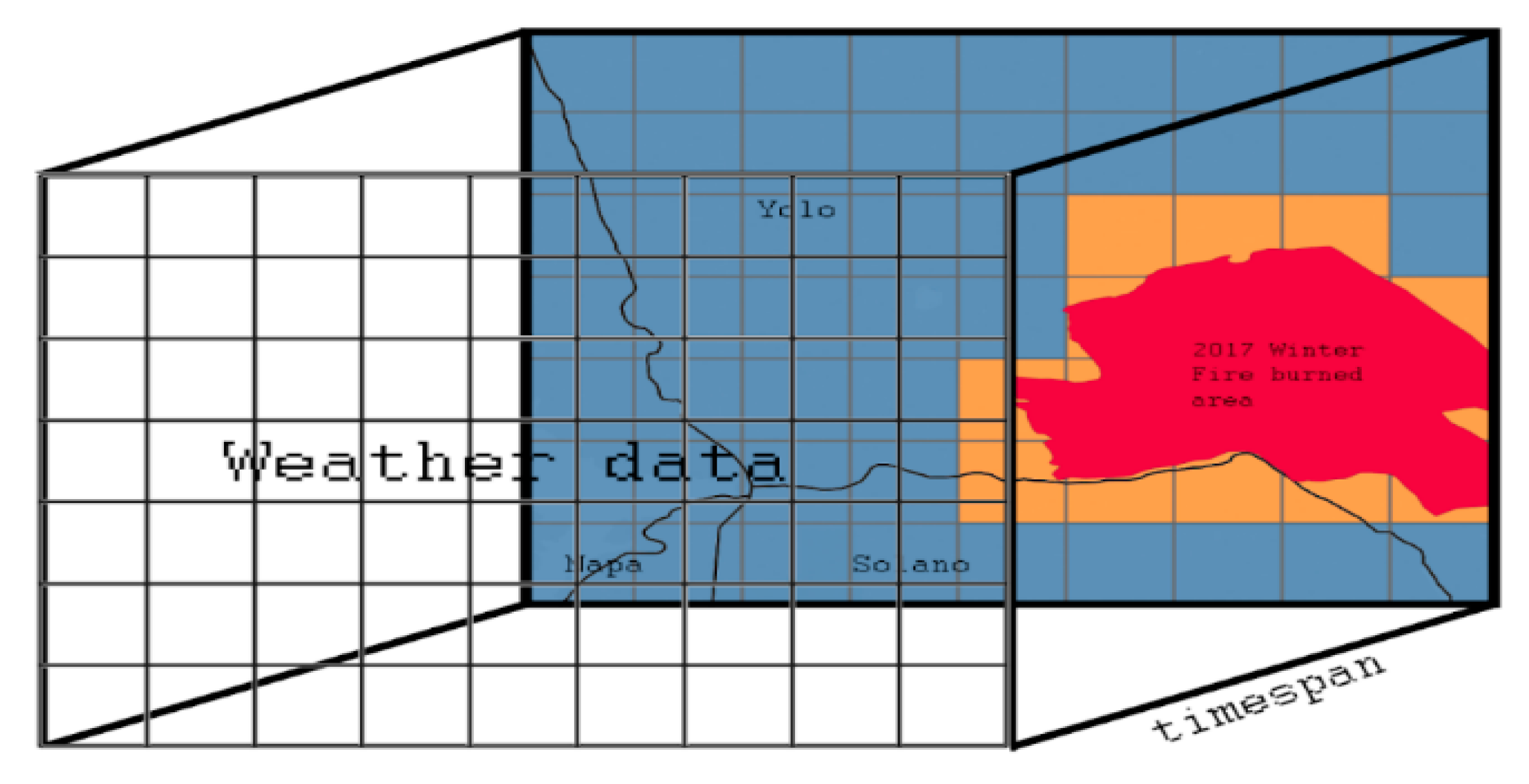
To create the weather dataset for the models, the selected area of study was divided into 1000 × 1000-m2 grid cells using free and open-source tool QGIS (Geographic Information System) to visualize the fire perimeter in a map (Figure 2). Thereafter, a mesh or gridded square layer was embedded on the area to isolate a fire-prone region/s, and coordinates of the grids were downloaded to be mapped with the weather data. To keep the data balanced for each sample of fire start day’s weather data, another sample from a no-fire day’s weather data was added to the dataset, and various combinations of years were included as well.
C. 
Vegetation data processing
For vegetation data, Landsat 8 dataset was gathered based on the area of interest geometry, and three separate GEE (Google Earth Explorer) data products applied on the image collection to derive NDVI (Normalized Difference Vegetation Index) [22,23,24], EVI (Enhanced Vegetation Index), and NDWI (Normalized Difference Water Index) vegetation indices. In order to overlay the vegetation indices in the area of study grid, the area was segmented into grids (1 km × 1 km) using the grid endpoints. Thirteen points including the four corners, four midpoints, centroid, and four diagonal points (or midpoints of four squares enclosed in the original square) were isolated. Vegetation indices of each of these points were directly fetched from GEE. Thereafter, the value for each grid was calculated as the average value of the 13 points after a series of experiments sampling 1, 5, and 13 points per grid. An elaborate analysis of this sampling methodology revealed that 13-point sampling per grid is sufficient and represented the vegetation of this area quite accurately. Taking all available points in the grid, features such as bodies of water can completely skew the calculation. For example, if half of a grid is a body of water, the other half with land can catch fire due to thick vegetation. For this reason, a 13-point approach for fire risk prediction was ideal compared to total aggregation of point-wise vegetation indices.
As part of data cleaning, we grouped points based on point id, start and end date and calculated the mean value such that a single value/row remains for a single inner grid at a given time. We integrated the original grid table with geometry, left, right, top, and bottom coordinates. Thereafter, the missing values were imputed. We considered using ‘time’ and ‘linear’ interpolation deemed most suitable for the time-series null value imputation [25]. The mathematical formula and Landsat bands-based formula for calculating Vegetation Index such as Normalized Difference Vegetation Index (NDVI), Enhanced Vegetation Index (EVI), and the Normalized Difference Water Index (NDWI) is given below in Equations (1)–(6) respectively [26]. NIR stands for Near-infrared band, whereas SWIR is a shortwave infrared band. The L value in EVI formula adjusts the canopy background, whereas the C value is the coefficient of atmospheric resistance. B is a blue band and G is the gain factor [27].
Formula for NDVI
NDVI = (NIR − Red) / (NIR + Red)
Landsat 8: NDVI = (Band 5 − Band 4) / (Band 5 + Band 4)
Range: −1 to 1
Formula for EVI
EVI = G * ((NIR − Red) / (NIR + C1 * Red − C2 * B + L))
Landsat 8: EVI = 2.5 * ((Band 5 − Band 4) / (Band 5 + 6 * Band 4 – 7.5 * Band 2 + 1))
Range: −1 to 1
Formula for NDWI
NDWI = (NIR − SWIR) / (NIR + SWIR)
Landsat 8: NDWI = (Band 5 – Band 6) / (Band 5 + Band 6)
Range: −1 to 1
In order to make the data balanced in terms of fire days vs. no-fire days, Synthetic Minority Oversampling Technique (SMOTE) [28] was used to generate the synthetic data to oversample the minority class (fire-days).
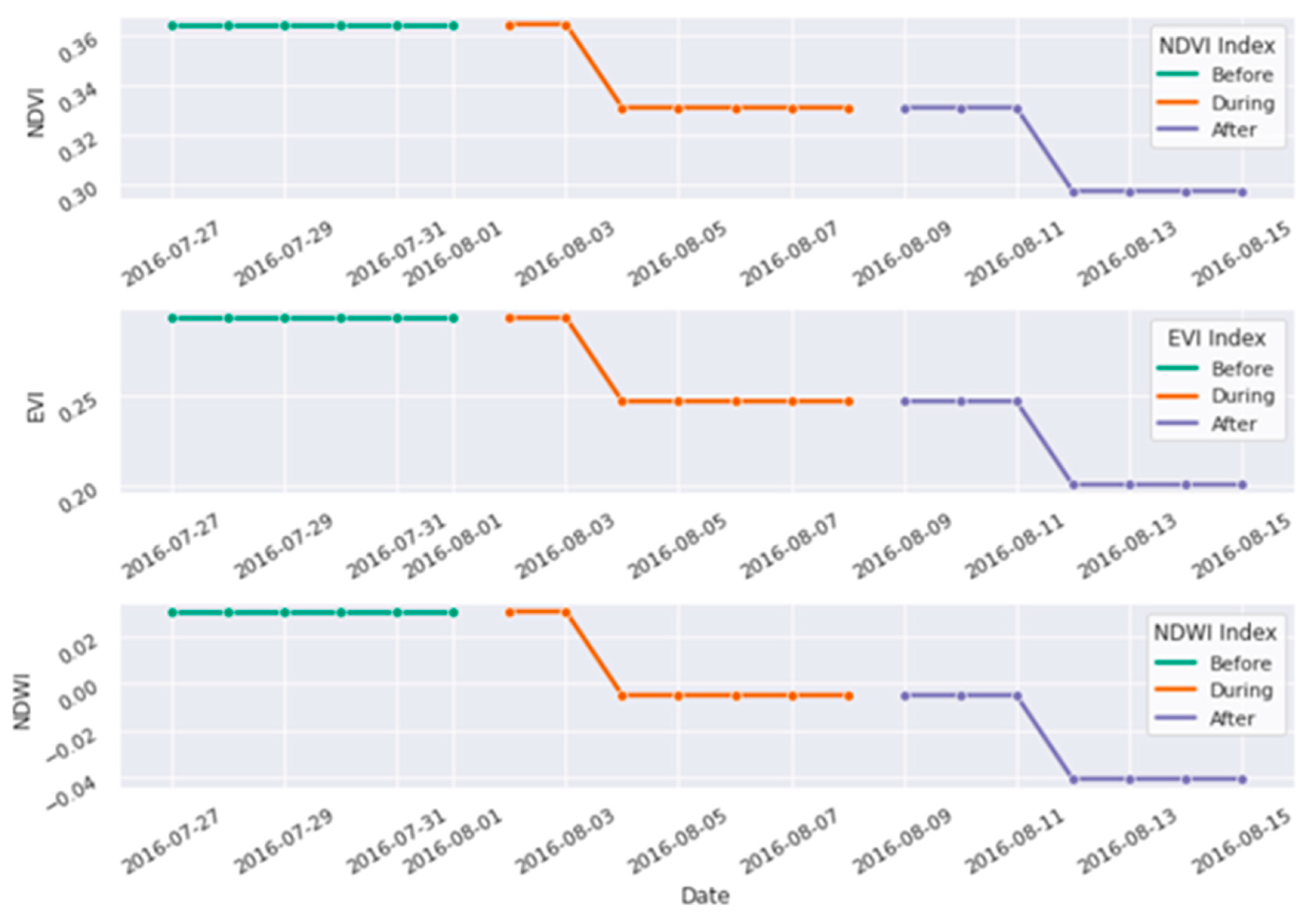
To display the fire probability of each of these indices, we chose a small subset of data before and after the fire, then set the data points before the fire to 1 (fire expected) and after the fire to 0 (No Fire). NDVI and EVI are reliable indicators of the likelihood of fire. The mean NDVI is 0.304 with a standard deviation of 0.148, whereas the mean EVI is 0.302 with a standard deviation of 0.111. Mean NDWI is 0.107 with a standard deviation of 0.135. Figure 3 shows the vegetation indices data before, during, and after the fire for one of the grid cells (id#25), which indicates the totally different ranges for the NDVI, EVI, and NDWI before, during, and after the fire.
D. 
Powerline data processing
The theoretical reason for using powerline dataset was that, although it does not provide enough information on wildfire prediction, it is a major factor in modeling wind direction and micro weather conditions to predict wildfire ignition. Powerline dataset alone lacks in temporal information since it does not change frequently. Combining with the weather dataset, it is effective in correlating the wildfire ignition conditions (powerline related fires usually occur during the windy weather).
We merged the spatial vector layers file with fire history and bounding box grid using the tools in QGIS software and exported the resultant data as a flat file. After exporting the flat file grids with no powerline passing through, it ended up having null values. For all the columns except Status and Circuit, null values were replaced with zero as the powerlines were not going through those grids. However, Status column null values were replaced as “Not operating” and, for Circuit column, null values were replaced with “Other” as the categorical variables.
E. 
Terrain data processing
For terrain data, 1-m Digital Elevation Models (DEM) maps were downloaded from USGS (U.S. Geological Survey) National Map 3DEP Downloadable Data Collection, merged with fire history data, and overlaid onto the study area bounding box grid using the inbuilt zonal statistics algorithm in QGIS. Then, we calculated the statistics for three features (slope, hill shade, aspect) in each grid and used them as the input to the machine learning algorithm.
Slope: Slope represents the rate of change of elevation for each digital elevation model (DEM) cell. It is the first derivative of a DEM, and by default, the slope appears as a grayscale image. We can add the Colormap function to specify a color scheme. The inclination of the slope can be output as either a value in degrees or percent rise utilizing these three options:
(1)
Degree: The inclination of the slope is calculated in degrees. The values range from 0 to 90.
(2)
Scaled: The inclination of the slope is calculated the same as degrees, but the z-factor is adjusted for scale.
(3)
Percent Rise: The inclination of the slope is output as percentage values. The values range from 0 to essentially infinity. A flat surface is 0 percent, and a 45-degree surface is 100 percent, and as the surface becomes more vertical, the percent rise becomes increasingly larger.
Hill Shade: To get a better look at the terrain, it is possible to calculate a hill shade, which is a raster that maps the terrain using light and shadow. A hill shade can provide very useful information about the sunlight at a given time of day, and it can also be used for aesthetic purposes to make the map look better.
Aspect: Aspect is the compass direction that a slope faces. After applying 1 × 1 km grid, statistics of the slope, hill shade, and aspect are calculated for each grid on the map.
We excluded the data for year 2014 from our model experimentation as weather data was missing for the same in dataset. With the four years of data available, we experimented with subsets of data for fitting and building the model as shown in Table 3. Combination of different years from the above types, along with stratified samples, were considered in model building after statistically analyzing the samples. The mentioned data sources, along with stratified samples, were combined and considered for model training, validation, and test datasets. Eighty percent and twenty percent of the dataset is used as training and test dataset, respectively. Furthermore, the training dataset is divided into 4:1 ratio for training and validation datasets.
Shown in Figure 4a,b are the most important features for the finalized training dataset in regard to base model I and base model II of the ensemble model, respectively. Figure 4c shows the same for combined model. The merits of our proposed model and the steps it uses to predict risk are as follows.

3. Wildfire Risk Prediction Models

In this section, we first formally discuss the merits of the proposed models, then explain the steps of our proposed risk prediction models in detail. We have already discussed the limitations of traditional and current machine learning models in the introduction section. Here, we will discuss the merits of our proposed models in brief. We have developed the models with the hourly or bi-weekly data for region-based wildfire risk prediction with augmented spatial sensitivity. Unlike the mentioned recent work in introduction section on wildfire models, we need a model that deals in wide range of variables such as weather, vegetation indices, terrain, and powerlines data, with both the spatial and temporal dimensions to address the practical wildfire challenges posed by the frequent fluctuations in weather forecast and region-based risk prediction. Hence, we used data-driven machine learning models that run on comprehensive datasets with multiple parameters including location-based weather, terrain, vegetation, and powerlines data, along with the fire history data to predict fire risk in our study area based on satellite data.
The high-level architectures of our proposed ensemble and combined machine learning models that ingest grid-based values are discussed in the following sections. The ensemble model stacks the best models, whereas the combined model runs on a combined dataset using the best-performing algorithm. As we have multiple layers of complex data sources, we decided to extract grid-specific data for the parameters in our study area to make the integration of datasets easier. The models proposed in this paper to predict the wildfire risk are the ensemble and combined models that run on comprehensive datasets with multiple parameters including location-based weather, terrain, vegetation, and powerlines data, along with the fire history data.
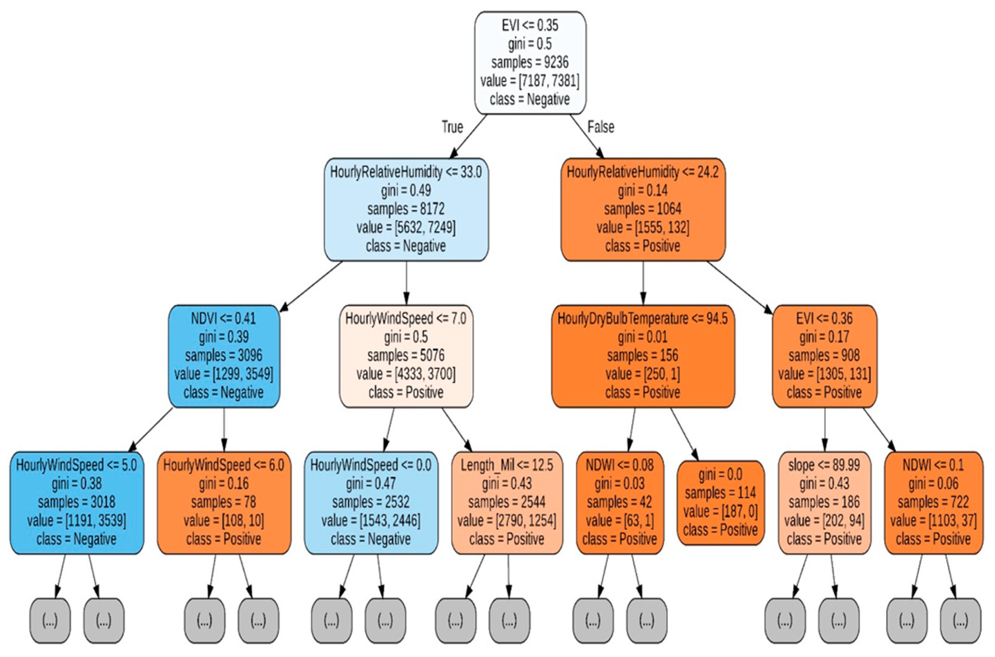
Unlike other existing models, these models are integrated models powered by machine learning algorithm such as Adaboost, Decision trees, Gradient descent, Multi-layered perceptron, Random Forest Tree (RF), and Long Short-Term Memory (LSTM) to address convoluted location-specific wildfire risk prediction. In terms of accuracy of individual models, the Random forest algorithm outperformed all other algorithms when experimented with varied target labeling and subsets of the datasets (refer Table 3). Thus, random forest was an optimal choice for the ensemble and combined wildfire risk predicting models (refer to Figure 5 for the random first tree visualization).
Accuracy comparison among machine learning with hyper-parameters are represented in Table 4. The Random Forest algorithm generally has better performance than decision trees. This is due to the Random Forest algorithm being an ensemble of decision trees. Thus, we employed Random Forest on the collected dataset for predicting the wildfire risk.
There are two main advantages of using Random Forest. First, the algorithm handles both numerical and categorical data, which allows more options on the choice of features. Second, since a random forest algorithm aggregates a collection of decision trees, it limits overfitting to a great context.

3.1. An Ensemble Model

In this section, we present an ensemble model, two base (weak) random forest algorithms used on a different set of data sources and their predicted probabilities combined to ensemble with stacking. For the first base model, data features included weather, powerline, and terrain data chose 8-day composites of vegetation indices available in Google Earth Engine (GEE) cloud catalogs as image collections for data ingestion.
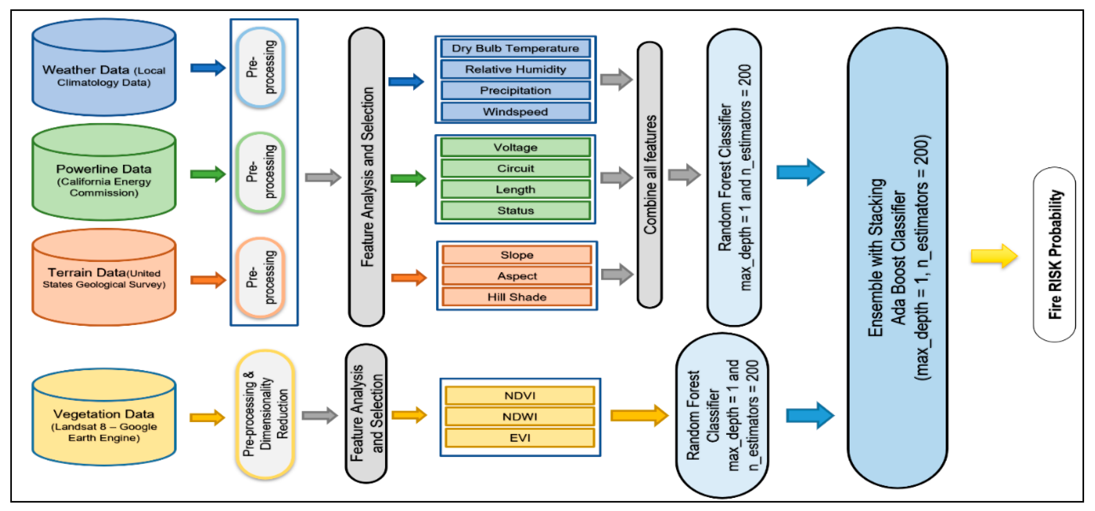
Weather, terrain, and powerline data were sparse and lacked sufficient temporal variation. Hence, they were clubbed together to produce the time series data for the base model. Figure 6 shows the architecture of the Ensample model. Data from each source (i.e., Weather, Powerline, Terrain, and Vegetation) were pre-processed, analyzed, and selected as part of the data transformation step. They were then inputted into two different random forest classifiers in order to calculate the wildfire risk probabilities from each, after which they were used in stacked generalization ensemble. In the stacked ensemble model, the outputs from the two weak models, called the base models (refer supplementary material for base models details and the interim results), were inputted to the meta classifier model resulting in a robust ensemble model.
During our experiments, Adaboost classifier consistently gave high accuracy as the second-layer learning algorithm for the ensemble model, although Random forest fared best in terms of accuracy. However, the results from the Random forest were inconsistent and unreliable. Therefore, we ensembled the models using the Adaboost meta estimator for the two base models with random forest classifier.
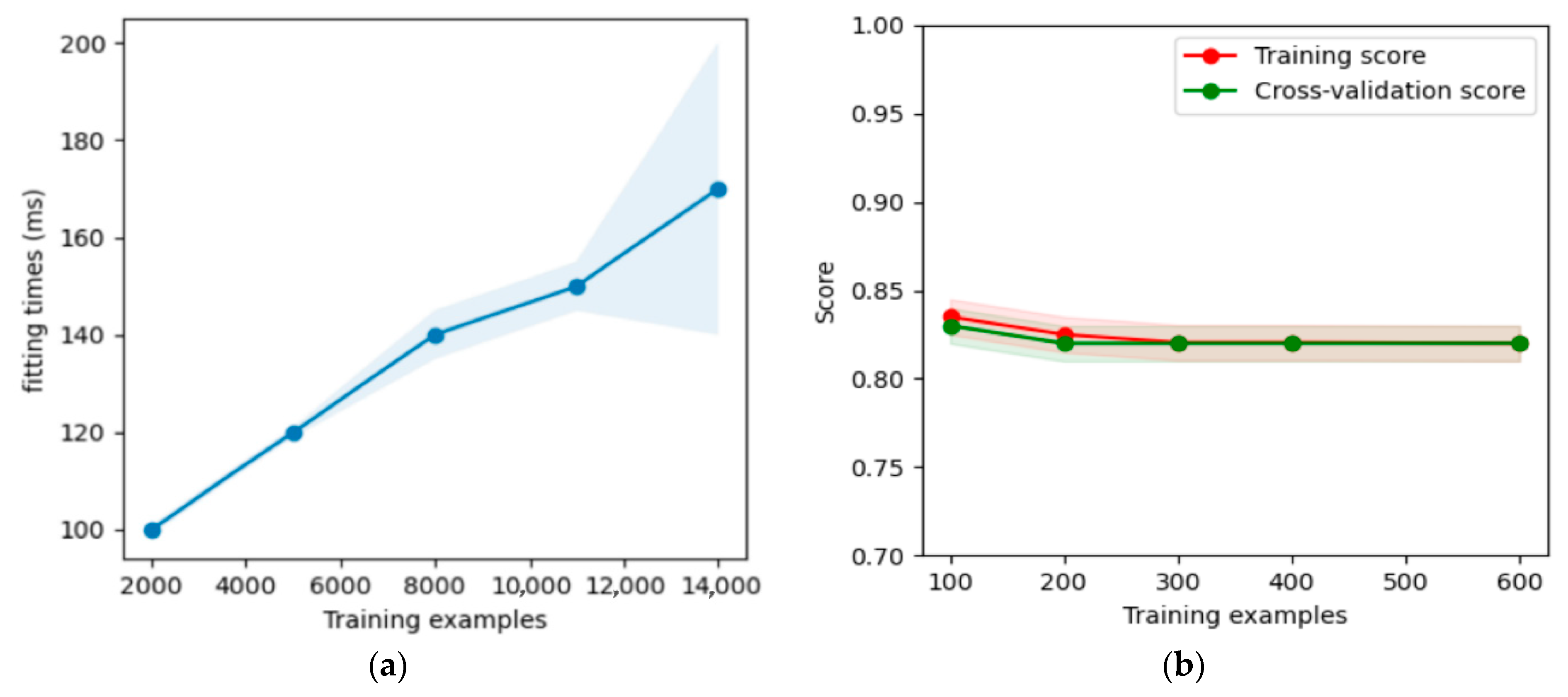
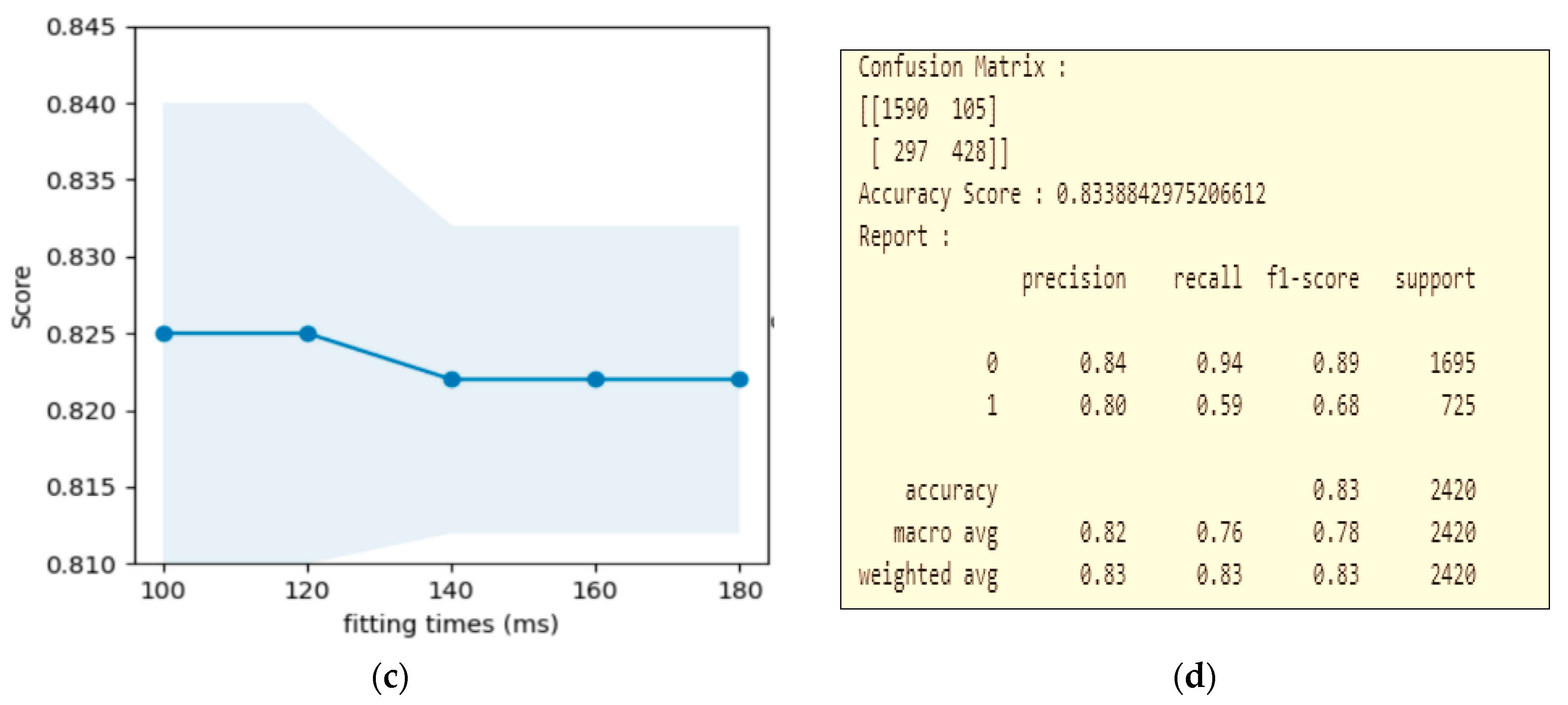
The above-mentioned individual vegetation and weather models were stacked, and their output was used as input for the final ensemble model. The learning curve in terms of the scalability of the model (fitting time vs. # of training examples) for the ensemble model is shown in Figure 7a. The ensemble model with “base model I” and “base model II” with combined output converged obtained a cross-validation accuracy of ~84% as shown in Figure 7b. This score is higher than what was obtained from the weak models alone.
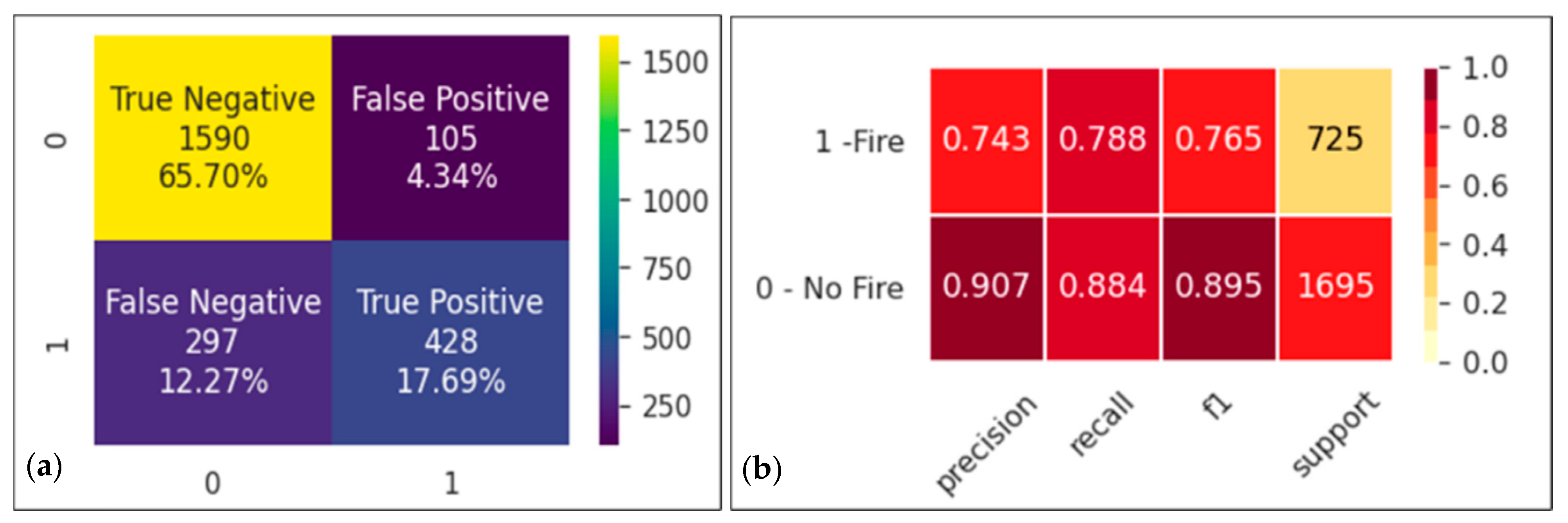
Overall, precision, recall, and f1 score were marked in the range of 80–84% as shown in Figure 8a,b, but ratio tp / (tp + fn) dropped to 59% for the samples with wildfire risk in Figure 7d. Figure 7c shows the performance curve with an accuracy of ~82%. For negative test data, the ensemble model resulted in a precision of 0.84 and an f1-score of 0.89 with support of 1695. For positive test data, the reported results were a precision of 0.80, an f1-score of 0.68, and a support of 725.
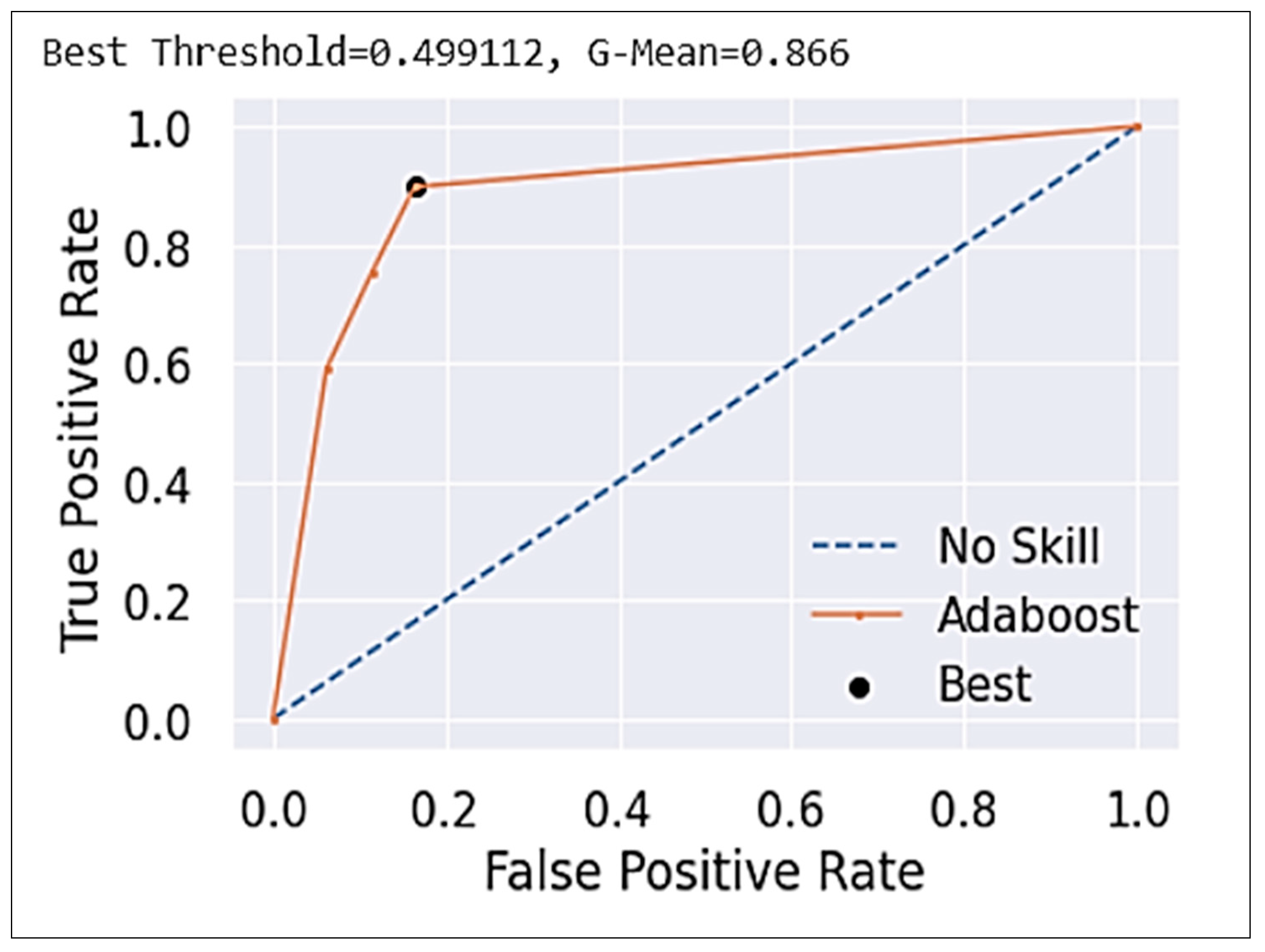
The ROC curve for the ensemble model is shown in Figure 9, which compares the true positive rate to the false positive as the threshold for predicting ‘1’ change. The area under the ROC curve is inherently related to the accuracy, but the AUC-ROC is preferred because it is automatically adjusted to the baseline and gives a robust picture of how the classifier performs at different threshold choices. It also shows the best threshold and ensemble model results with modified threshold value. The ROC curve shows the best threshold of 0.499112 and a G-Means of 0.866.

3.2. Combined Model

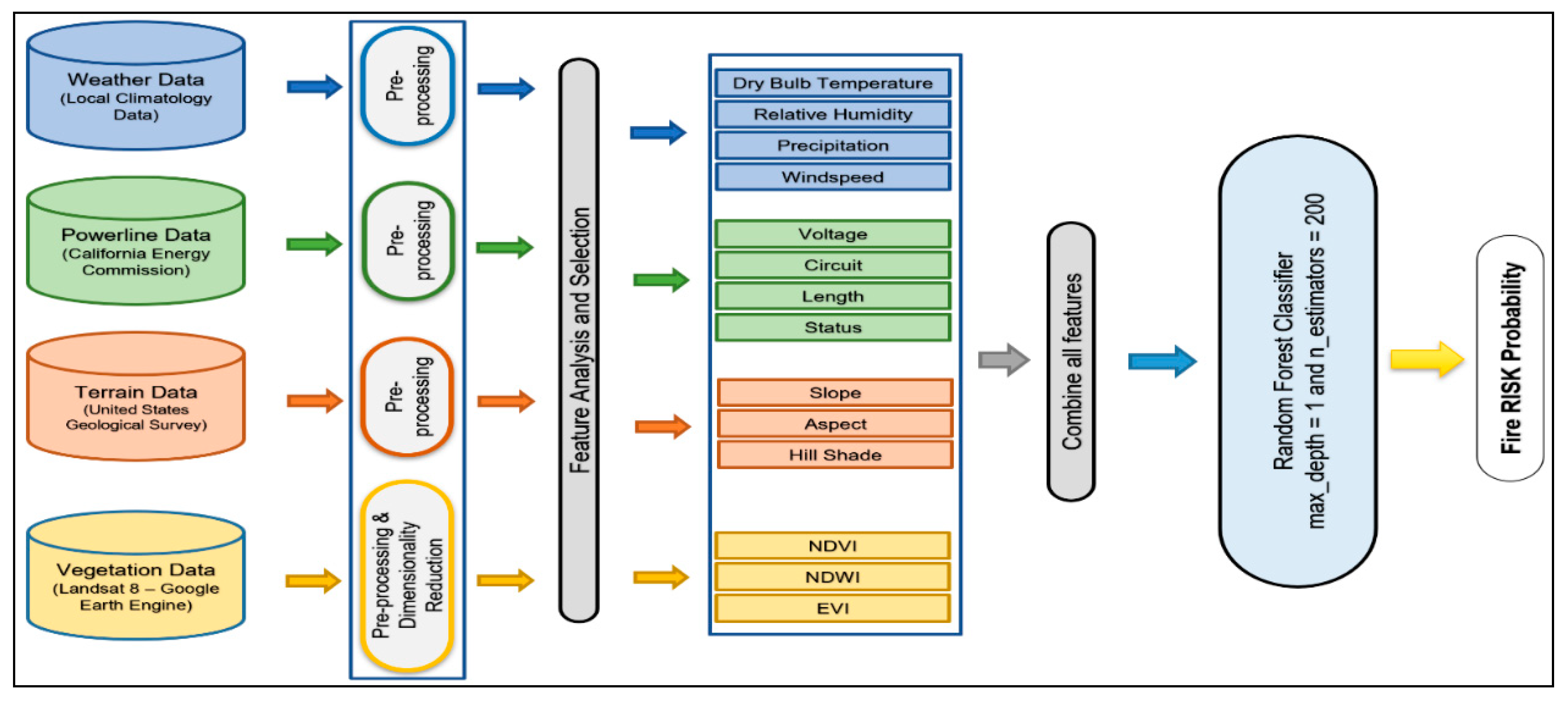
As seen in the diagram above (Figure 10), data from each source (i.e., Weather, Powerline, Terrain, and Vegetation) combined as data features and placed into a random forest classifier. The combined dataset with all the parameters such as weather, vegetation, terrain, and power lines were utilized for training with Random forest classifier and stratified train test split fared best. Data before being ingested were pre-processed, analyzed, and selected as part of data transformation step, and then combined and ingested into random forest classifier, which in turn calculates the wildfire risk probability. For both the models (i.e., ensemble and combined models), the same hyperparameters settings, which are max_depth as 1 for the tree in the random and n_estimators as 200, worked best. The combined dataset with all the parameters such as weather, vegetation, terrain, and power lines, in a python dataframe format, was utilized for training various models. Training, test, and validation sets following a similar methodology as the weather dataset. Yet again, the type II dataset (from Table 3) with random forest classifier and stratified train test split fared.
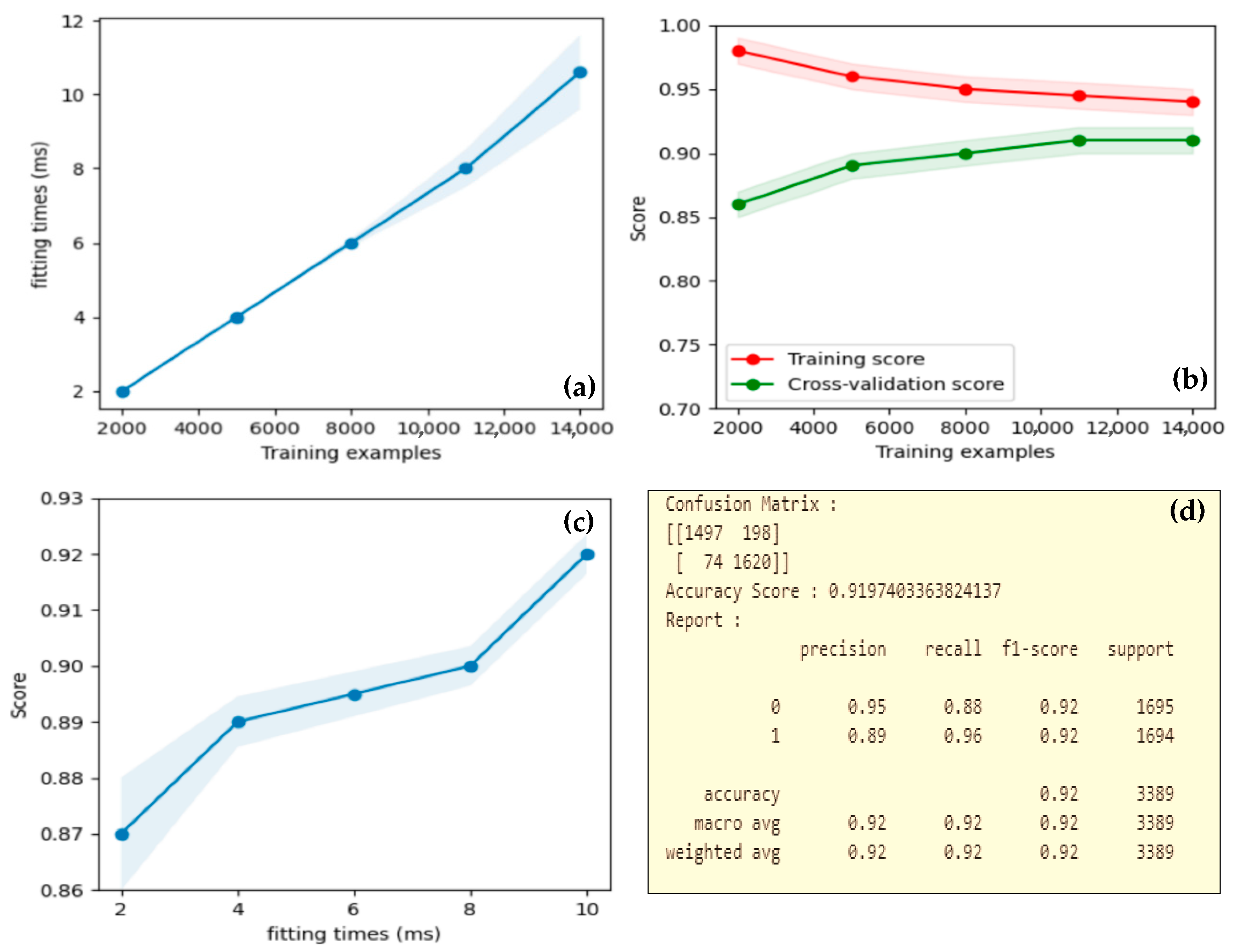
Learning curve in terms of the scalability of the model (fitting time vs. #training examples) for the ensemble model fitted with combined data (weather, terrain and powerline model, and vegetation model) are shown in Figure 11a.
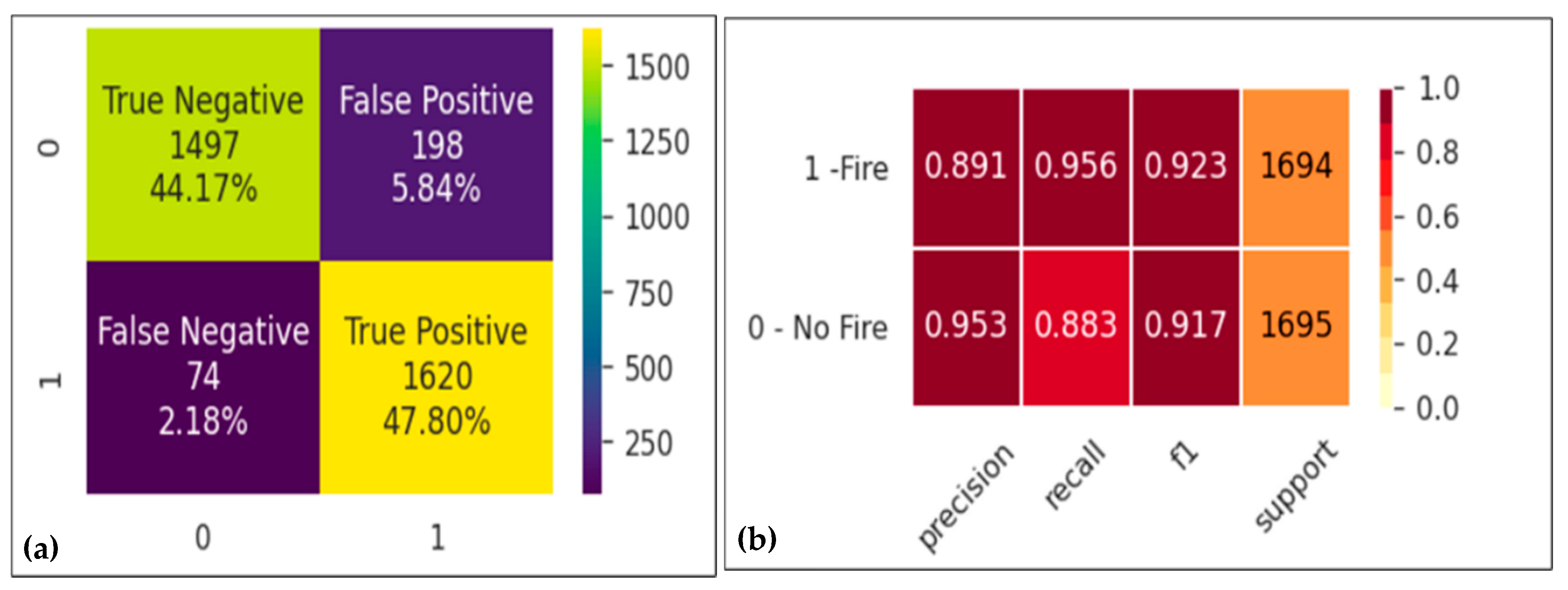
Figure 12a,b show the classification report, accuracy, and confusion matrix for the combined model. Clearly, combined random forest model has better evaluation results compared to ensemble model and the achieved model accuracy is 91%. Figure 11c shows the performance curve for the combined model. With the weather, vegetation, power lines, and terrain data being major parameters used in predicting fire risk, we tried different combinations of the data and models to get the best fit. The classification also shows the percentage for precision, recall, and f1 score for all classes. The classification report for the combined model shows balanced results with 0.95 precision and 0.92 f1-score with 1695 support for positive and 0.89 precision and 0.92 f1-score with 1694 support for negative test data. The dataset with all the above-mentioned parameters together was used to build one variation of the machine learning model. We called it a combined model that could fetch a model with 92% accuracy. This is by far the best model we obtained in terms of the evaluation results. Evaluation metrics for the combined model is shown in Figure 11d. Further, we tested it on a newer validation dataset (refer Figure 11b) and obtained good results. Thereafter, this robust model was considered as the final machine learning model for this project. The combined model, compared to the ensemble model, does a fantastic job in identifying the true negatives and true positives (i.e., 92% of the times it predicts the true negatives and true positives correctly). Out of the remaining 8%, false positives are close to 5.5%, and at the same time false negatives are approximately 2.5%.
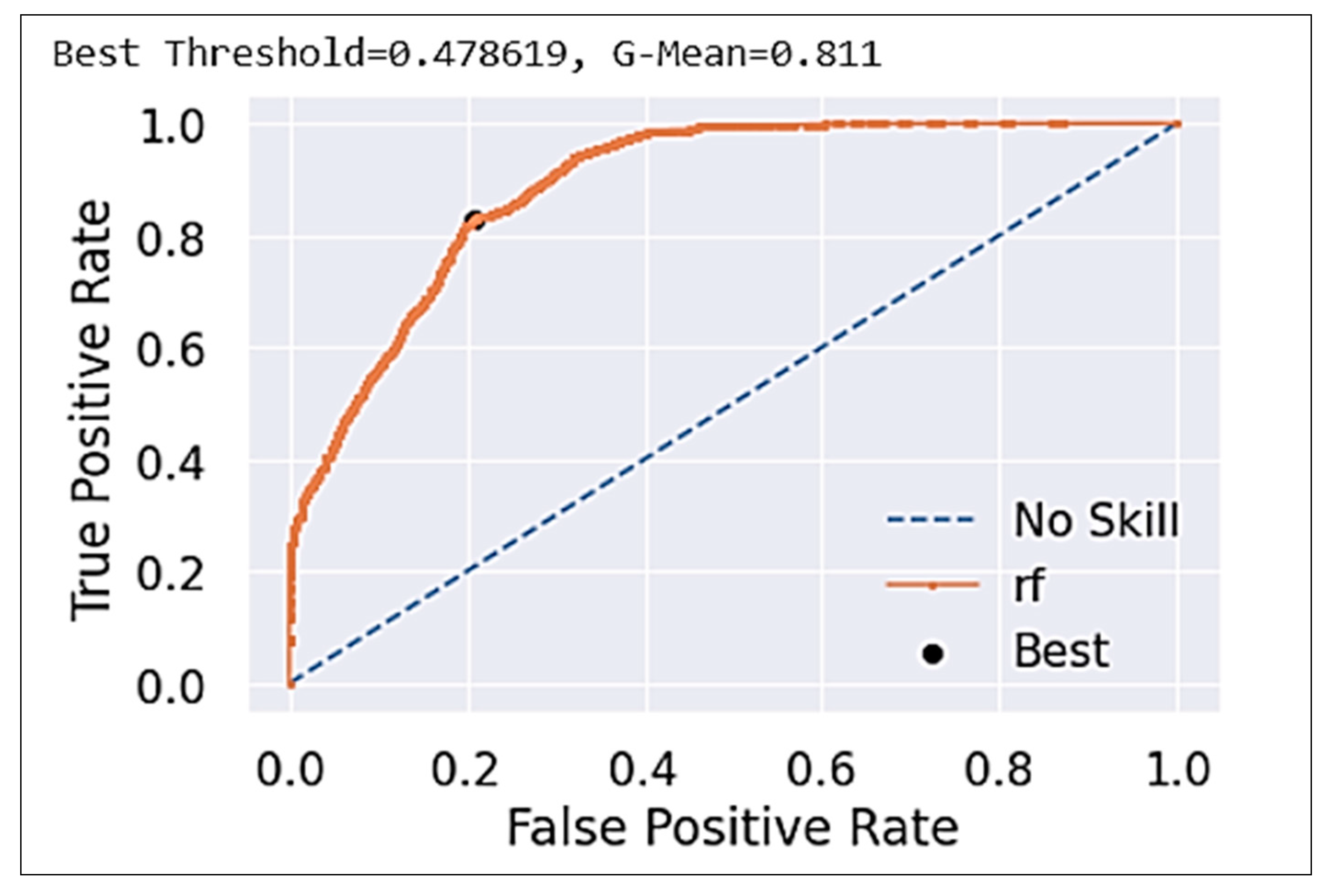
The ROC curve was plotted and evaluated, with the best threshold of 0.478619 and a G-Means of 0.811. The image in Figure 13 shows the best threshold and combined model results with a modified threshold value.
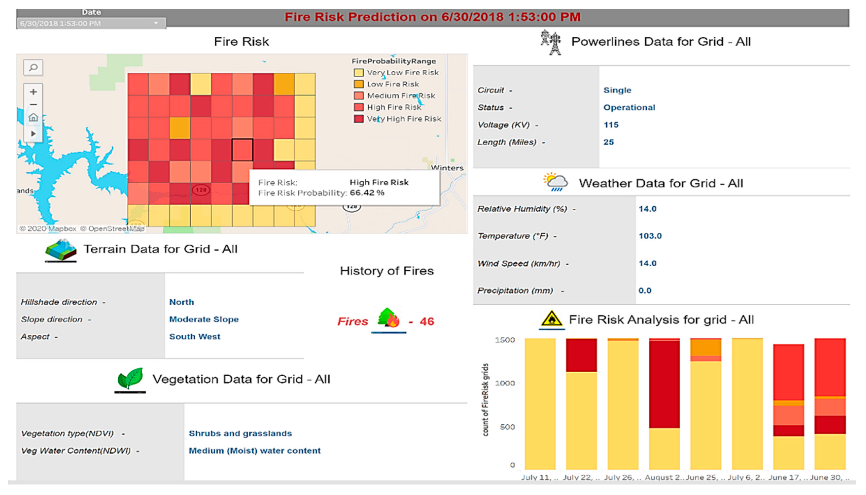
Figure 14 shows a combined model prediction dashboard for the real-time prediction of wildfire risk for the area under study on 6/30/2018 along with terrain, powerlines, vegetation, and weather data values. The top left part displays all the grid cells for the area under study. Color-coded grids represent the fire risk probabilities for each of the grids individually based on the spatial and temporal conditions. The above figure visualizes the fire risk probability and the risk label on a chosen date. The fire risk is lower on southern and eastern boundaries on that particular day, mainly based on the calculated vegetation indices values and terrain conditions as the Eastern and Southern area is not fertile and has no vegetation that can lead to wildfire. However, the high risk on a particular date is due to a combination of vegetation, weather, terrain, along with the powerline data. Regions close to water may have lush vegetation that causes the heightened fire risk. If the weather conditions are dry, that provides an abundance of combustible fuel.

4. Conclusions

In this era of climate change and rising temperatures, blazing wildfires are becoming a year-round phenomenon [2]. Wildfires, also known as wildland fires, forest fires, or brush fires, are uncontrolled fires sweeping across millions of acres of land, causing severe and extensive damage to our ecosystem [2]. With this study, we have established a machine-learning-ready basis for future studies and explored the key impacting features for wildfire prediction from a machine learning point of view. Unlike the statistical and machine learning approaches, our model relies on the high number of spatial and temporal variables and not just the standard ones such as weather, with which we learned the past fire events and obtained cutting-edge accuracy of 92% and real-time effectiveness in wildfire risk prediction.
In comparison to the ensemble model (Base model I + Base model II -> Adaboost), the combined model emerged as the winner in terms of accuracy. The results were not surprising but as expected; the justification for achieving better accuracy in the combined model is that Ensemble Base Model I (weather, terrain, and powerline) had no knowledge of the vegetation and, similarly, Ensemble Base Model II (vegetation) had trained separately and, due to whose vegetation model, could not derive any relation with the other variables. However, the combined model with a complete set of datasets was able to deduce the relationship among all the independent variables and achieved 92% accuracy.
In order to be successful in predicting the fire risk (including the ignition), high temporal resolution is needed. The model must be trained on region-specific variables such as vegetation, terrain, and weather datasets. With high spatial and temporal accuracy datasets, it can pinpoint an incident in real-time if we can fetch the most recent data. However, drawbacks were observed, the first one being that our machine learning model depends heavily on the data availability for the terrain. Additionally, other data such as weather, powerline, vegetation, and fire history are required. To further apply our model in different regions of the world, it relies on weather conditions and other region-specific temporal and spatial variables that add the region-specific constraints to the model’s hypothesis space and can attain better fire risk prediction accuracy.
Our models can be further improved to be generalized to all areas. For the future research direction, we are developing a wildfire machine learning platform to support wildfire risk analysis and prediction, as well as fire spreading prediction.

Author Contributions

Conceptualization, J.G.; methodology, A.M., M.R.R. and P.K.; software, V.A.K.T., N.P. and Q.L.; validation, M.R.R. and N.P.; data curation, Q.L., P.K. and V.A.K.T.; writing—original draft preparation, A.M.; writing—review and editing, A.M., J.G. and S.C.; supervision, J.G.; project administration, J.G. and S.C. All authors have read and agreed to the published version of the manuscript.

Funding

This research is partly supported by NASA MUREP (NNX15AQ02A).

Institutional Review Board Statement

Not applicable.

Informed Consent Statement

Not applicable.

Data Availability Statement

Publicly available datasets were analyzed in this study. This data can be found here: https://drive.google.com/drive/folders/1_3F12htWwtHFPxeyYx07Fly8Ts10hDYY?usp=sharing.

Acknowledgments

We want to thank Department of Applied Data Science, Department of Computer Engineering, and the Center for Applied Atmospheric Research and Education of San Jose State University, California, for providing us the opportunity to work on this project. Proofreading by Paul Zechiel was much appreciated. We also thank JustLight Technology Inc. for the grant support and SJSU Excellent Research Center on Smart Technology and Complex Systems for their support.

Conflicts of Interest

The authors declare no conflict of interest.

References

  1. Saleh, Y.; Hamid, R.P.; Sayed, N.M.; Soheila, P.; Saeedeh, E.; John, P.T. A Machine learning framework for multi-hazards modeling and mapping in a mountainous area. Sci. Rep. 2020, 10, 12144. [Google Scholar]
  2. World Economic Forum. Available online: https://www.weforum.org/agenda/2019/05/the-vicious-climate-wildfire-cycle (accessed on 9 May 2019).
  3. Calmatters. Available online: https://calmatters.org/explainers/californias-worsening-wildfires-explained/ (accessed on 20 August 2020).
  4. Scasta, J.; Weir, J.; Stambaugh, M. Droughts and Wildfires in Western U.S. Rangelands 2016, 38, 197–203. [Google Scholar] [CrossRef] [Green Version]
  5. California Department of Forestry and Fire Protection. Available online: https://www.fire.ca.gov/stats-events/ (accessed on 13 January 2021).
  6. Tiziano, G.; Bachisio, A.; Grazia, P.; Pierpaolo, D. An Improved Cellular Automata for Wildfire Spread. Procedia Comput. Sci. 2015, 51, 2287–2296. [Google Scholar]
  7. Bianchinia, G.; Caymes-Scutariab, P.; Méndez-Garabettiab, M. Evolutionary-Statistical System: A parallel method for improving forest fire spread prediction. J. Comput. Sci. 2015, 6, 58–66. [Google Scholar] [CrossRef]
  8. Miguel, M.G.; Germán, B.; Paola, C.S.; María, L.T. Increase in the quality of the prediction of a computational wildfire behavior method through the improvement of the internal metaheuristic. Fire Safe. J. 2016, 82, 49–62. [Google Scholar]
  9. Andrés, C.; Ana, C.; Tomàs, M. Applying Probability Theory for the Quality Assessment of a Wildfire Spread Prediction Framework Based on Genetic Algorithms. Sci. World J. 2013, 2013, 728414. [Google Scholar]
  10. Andrés, C.; Ana, C.; Tomàs, M. Response time assessment in forest fire spread simulation: An integrated methodology for efficient exploitation of available prediction time. Environ. Model. Softw. 2014, 54, 153–164. [Google Scholar]
  11. Andrés, C.; Ana, C.; Tomàs, M. Relieving Uncertainty in Forest Fire Spread Prediction by Exploiting Multicore Architectures. Procedia Comput. Sci. 2015, 51, 1752–1761. [Google Scholar]
  12. Philippe, J.G.; Guru, J.B.; BabuMagda, B. A Novel Visualization Environment to Support Modelers in Analyzing Data Generated by Cellular Automata, the Lecture Notes in Computer Science book series. In Proceedings of the International Conference on Digital Human Modeling and Applications in Health, Safety, Ergonomics and Risk Management, Toronto, ON, Canada, 23 June 2016; pp. 529–540. [Google Scholar]
  13. George, E.S.; Imad, H.E.; George, M.; Uchechukwu, C.W. Artificial Intelligence for Forest Fire Prediction. In Proceedings of the IEEE/ASME International Conference on Advanced Intelligent Mechanotrics, Montreal, ON, Canada, 6–9 July 2010. [Google Scholar]
  14. Onur, S.; Suha, B.; Cenk, D. Mapping regional forest fire probability using artificial neural network model in a Mediterranean forest ecosystem. Geomat. Nat. Haz. Risk 2016, 7, 1645–1658. [Google Scholar]
  15. Stojanova, D.; Kobler, A.; Ogrinc, P.; Ženko, B.; Džeroski, S. Estimating the risk of fire outbreaks in the natural environment. Data Min. Knowl. Discov. 2011, 24, 411–442. [Google Scholar] [CrossRef]
  16. Guruh, F.S.; Khabib, M. Predicting Size of Forest Fire Using Hybrid Model. In Proceedings of the Conference ICT-EurAsia 2014: Information and Communication Technology, Bali, Indonesia, 14–17 April 2014; pp. 316–327. [Google Scholar]
  17. Marcos, R.; Juan, R. An insight into machine-learning algorithms to model human-caused wildfire occurrence. Environ. Model Softw. 2014, 57, 192–201. [Google Scholar]
  18. Famiglietti, C.; Holtzman, N.; Campolo, J. Satellite-Based Prediction of Fire Risk in Northern California. Stanford University; Final Report, 2018. [Google Scholar]
  19. Salehi, M.; Rusu, L.I.; Lynar, T.; Phan, A. Dynamic and Robust Wildfire Risk Prediction System: An Unsupervised Approach. In Proceedings of the KDD ’16: The 22nd ACM SIGKDD International Conference on Knowledge Discovery and Data Mining, San Francisco, CA, USA, 13–17 August 2016. [Google Scholar]
  20. Dutta, R.; Das, A.; Aryal, J. Big data integration shows Australian bush-fire frequency is increasing significantly. R. Soc. Open Sci. 2016, 3, 150241. [Google Scholar] [CrossRef] [PubMed] [Green Version]
  21. Fire Perimeters GIS Data, California Department of Forestry and Fire Protection. Available online: https://frap.fire.ca.gov/frap-projects/fire-perimeters/ (accessed on 13 January 2021).
  22. NAIP Imagery, United States Department of Agriculture from Service Agency. Available online: https://www.fsa.usda.gov/programs-and-services/aerial-photography/imagery-programs/naip-imagery/ (accessed on 13 January 2021).
  23. Staff, S.X. Proba-V images Portuguese forest fire. Phys. Org. 2017.
  24. El-Nesr, M. Filling Gaps of a Time-Series Using Python. Medium. Available online: https://medium.com/@drnesr/filling-gaps-of-a-time-series-using-python-d4bfddd8c460 (accessed on 31 December 2018).
  25. Landsat Science, NASA. Available online: https://landsat.gsfc.nasa.gov/landsat-8/ (accessed on 20 February 2020).
  26. NDVI, NDBI & NDWI Calculation Using Landsat 7, 8. Asian Institute. Available online: https://www.linkedin.com/pulse/ndvi-ndbi-ndwi-calculation-using-landsat-7-8-tek-bahadur-kshetri/ (accessed on 30 September 2018).
  27. Landsat Surface Reflectance-Derived Spectral Indices. USGS. Available online: https://www.usgs.gov/media/images/landsat-surface-reflectance-and-enhanced-vegetation-index (accessed on 13 January 2021).
  28. Brownlee, J. SMOTE Oversampling for Imbalanced Classification with Python. Machine Learning Mastery. 17 January 2020. [Google Scholar]
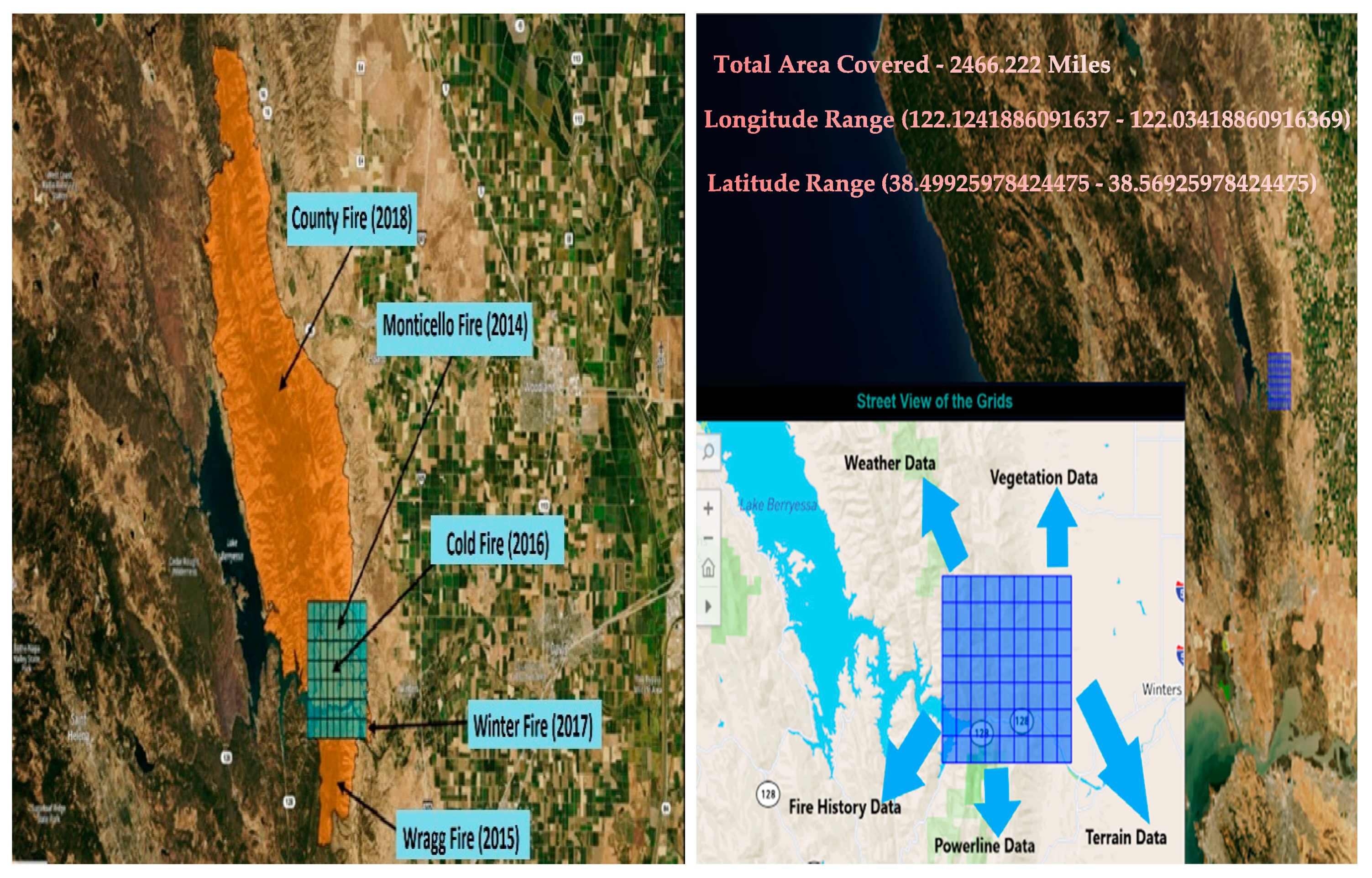
Figure 1. Integration of study area and Fire History (Monticello and Winters, California).
Atmosphere 12 00109 g001
Figure 2. Data mapping design for Base model I.
Atmosphere 12 00109 g002
Figure 3. Before, During and After fire, data w.r.t. vegetation indices for a grid cell id#25 in 2016.
Atmosphere 12 00109 g003
Figure 4. Feature importance for weather, powerline, and terrain dataset (a), vegetation dataset (b), and combined dataset (c).
Atmosphere 12 00109 g004
Figure 5. Generated random forest tree for weather, terrain, vegetation, and powerlines data.
Atmosphere 12 00109 g005
Figure 6. Architecture of the Ensemble (Adaboost) Random Forest models.
Atmosphere 12 00109 g006
Figure 7. Final Ensemble model (Adaboost)—Scalability (a), Learning Curve (b) on Training examples, Performance Curve (c), and Evaluation metrics (d).
Atmosphere 12 00109 g007aAtmosphere 12 00109 g007b
Figure 8. Confusion Matrix (a) and Classification report (b) of for Ensemble (Adaboost) model.
Atmosphere 12 00109 g008
Figure 9. ROC Curve for Ensemble (Adaboost) random forest model.
Atmosphere 12 00109 g009
Figure 10. Architecture of the Combined dataset Random Forest model.
Atmosphere 12 00109 g010
Figure 11. Combined dataset model (Random Forest)—Scalability (a), Learning Curve (b) on Training examples, Performance Curve, (c) and Evaluation metrics (d).
Atmosphere 12 00109 g011
Figure 12. Confusion Matrix (a) and Classification report (b) of Combined Random forest model.
Atmosphere 12 00109 g012
Figure 13. ROC for Combined random forest model.
Atmosphere 12 00109 g013
Figure 14. Fire Risk Prediction on 6/30/2018.
Atmosphere 12 00109 g014
Table 1. A Comparison of Machine Learning Models in Wildfire Risk.
Paper IDRegionPurpose and Area of StudyML ModelAccuracy
(in Percentage)
Data Params
Fire HistoryWeatherLandOther
Famiglietti, C., et al. (2018) LebanonFire Risk predictionSVM96.00%Daily Number of FireTemperature, Humidity, Solar radiation, PrecipitationN.A.N.A.
Dutta, R., et al. (2016)SloveniaFire outbreak predictive modelIBk80.50%Fire HistoryTemperature, Humidity, Wind Speed, Solar radiation, Precipitation, Transpiration & Evaporation, Weather ForecastLand usages, Altitude, Soil MoistureTraffic Corridor, Settlement Map
NB81.00%
J4878.60%
JRip81.50%
LogR83.00%
SVM83.00%
AdaBoost83.30%
BagJ4884.90%
RF82.50%
Bnet81.70%
NB55.32%
DT86.07%
RF66.69%
KNN86.08%
SVM91.31%
BRT73.00%
SVM70.90%
LR68.60%
El-Nesr, M. (2018)Blue Mountains, Australia Fire risk predictionCBFR85–90%Daily Number of FireN.A.ElevationN.A.
NASA (2020)AustraliaWildfire hotspot predictionKNN91.76%Fire HistoryHumidity, Wind Speed, Solar radiation, Transpiration and Evaporation, Heat Flux, Vapor PressureSoil MoistureN.A.
Bagging Tree94.53%
Ensemble91.00%
Our ModelMonticello and Winters, CaliforniaWildfire risk predictionRF91.76%Fire History, Daily Number of firesTemperature, Humidity, Precipitation, Wind Speed, Wind, Rain, Weather forecastSlope, Hill-shade, AspectVegetation Indices, Remote sensing, Powerline
Ensemble91.00%
Abbreviations: SVM (Support Vector Machine), MLP (Multilayer Perceptron), KNN (k-Nearest Neighbors), IBk (instance-bases learning with parameter k), NB (Naive Bayes), J48 (J48 Decision Trees), JRip/RIPPER (Repeated Incremental Pruning to produce error reduction), LogR (Weighted Decision Trees), RF (Random Forest), LR (Logistic Regression), BP (Back Propagation), CBFR (Context-Based Fire Risk), BRT (Boosted Regression Trees), BN (Bayesian Networks), Bnet (Tree Augmented Naive Bayes), N.A. (Not applicable).
Table 2. Data types and their sources.
DataData TypeSourcesTime Range
Fire HistoryShape fileFire and Resource Assessment Program (FRAP), CAL Fire, United States Forest MSDA Project, Service region, Bureau of Land Management, and National park service2015–2018
WeatherCensor data (CSV file)Climate Data Online (CDO) and Local Climatology Data (LCD)2015–2018
VegetationRemote-sensing satellite dataLandsat 8 satellite using Google Earth Engine (GEE)2014–2019
PowerlineShape fileCalifornia Energy CommissionN.A.
TerrainDEM fileUnited States Geological Survey (USGS)N.A.
Table 3. Variation of dataset for model building and training.
Data UsedPositive Target DataNegative Target Data
Type IData during fire7 Days before fire
Type IIData on fire start dateData before the fire
Type IIIData before fireData after fire
Type IVData on fire start date, excluding no-fire gridsData before the fire, excluding no-fire grids
Table 4. Model Accuracy with different ML algorithms.
ModelAccuracyHyper-Parameters Used
Random Forest92n_estimators = 200
Adaboost91.5n_estimators = 50, learning_rate = 1
Gradient Boosting trees90.5loss=deviance, n_estimators = 100
Weighted Decision Trees89.1criterion = gini,
splitter = best
MLP86.1activation = Softmax,
solver = adam
LSTM91.6Dropout = 0.2,
activation = Softmax
Publisher’s Note: MDPI stays neutral with regard to jurisdictional claims in published maps and institutional affiliations.