Temperature Response from the Change of Surface Heat Flux and Vertical Diffusivity by Urbanization

Abstract

A 1-D diffusion model of temperature is employed to understand important features of temperature response to the changes of surface heat flux (SHF) and vertical diffusivity shown in 3-D model simulations. Analytical results show that the temperature response to the SHF change is the convolution of the SHF change and Green’s function (GF). Because the GF is inversely proportional to the square root of diffusion coefficient near the surface, weak/strong diffusivity in the early morning/noontime tends to generate a large/small temperature response by slowing/accelerating heat flow from surface to the atmosphere. The modulation effect of the GF and the convolution effect explain very different temperature responses to the SHF change during each period. Analytical results also show that the temperature response to the change of DF is equal to the convolution of the product of diffusion coefficient change, vertical gradients of reference temperature and the GF. Because the vertical gradient of the GF is negative below 80 m, enhanced/reduced diffusivity would enhance/weaken the urban temperature, if the vertical gradient of reference temperature is negative/positive. Numerical results with typical values of the changes of SHF and diffusivity suggest that the changes of SHF has the dominant contribution to the temperature response.

1. Introduction

Large-scale urbanization significantly changes the land use and land cover in urban regions. The impervious surfaces of urban buildings, roofs and roads as well as the modified vegetation structure change the urban surface energy balance by altering the aerodynamic, radiative, thermal and moisture properties. The vertical diffusivity in urban areas is also changed by the change of surface heat fluxes as well as urban roughness length [1,2]. The impacts of these changes on the urban meteorological and chemical fields have been examined by employing the observation method [1,3,4,5], and by using high-resolution numerical models [5,6,7,8,9,10] implemented with urban schemes [11,12]. Among the meteorological fields affected by urbanization, the change of temperature near the surface, particularly the urban heat island (UHI) phenomenon, has been studied extensively because of its adverse impacts on human comfort and safety, urban ecology, as well as its indirect impact on urban climate through increasing energy demand in summer.

Although it has been recognized that the change of urban temperature is closely associated with the change of surface heat fluxes by urbanization, the mechanism underlying the diurnal temperature response to the change of surface heat flux has not been fully investigated. Observations [13,14] and model simulation results [10] show that the magnitude of the heat flux reduction in urban centers during the daytime in summer is about several times larger than that of heat flux enhancement in the early morning. However, the magnitude of the corresponding temperature change is much smaller than the 2 ${}^{°}$C to 3 ${}^{°}$C temperature enhancement—the so called UHI effect in the early morning. The cause of such drastically different response has not been investigated. In addition, it is also not clear how the change of vertical diffusivity by urbanization would affect urban temperature.

Because change of urban temperature is associated with interconnected physical and dynamical processes, it is difficult to assess the contribution of each process by examining the data of observation and model simulations. In this work, a 1-D diffusion model is employed to understand the drastically different temperature responses during the different period. There are several benefits of using the 1-D diffusion model. Unlike the numerical prediction model and climate model which cannot identify the impact of a specified process due to the interaction of many different processes in the model, the 1-D model can isolate the specified process and examine its contribution. Like other theoretical models used in atmospheric dynamics, the diffusion model has a simple form and its analytical solution can be derived. Because the model contains effects of surface heat flux and diffusivity, the solution can be used to show explicitly how temperature responds to the changes of surface heat flux and vertical diffusivity, and to examine their contributions by using the typical values of change of surface heat flux and diffusivity in numerical model simulations. Understanding the two contributions and corresponding mechanisms can help us gain physical insight into the diurnal and seasonal variations of the urbanization impact on urban temperature, and better interpret the numerical results of 3-D air quality model (GEM-MACH) of the Environment and Climate Change Canada [10,15]. Furthermore, the analytical results can help us understand the impacts of the uncertainties in surface heat flux associated with urban schemes and uncertainties in diffusion coefficient associated with diffusion parameterization schemes on the performance of numerical forecasts.

The paper is arranged as follows. A linearized diffusion equation around a reference state is presented first and the analytical solution to the equation is then derived in Section 2. Numerical results based on the analytical solution are shown in Section 3. A summary of the results is given in the last section.

2. 1-D Diffusion Model and Solution

Due to its simple form, the 1-D diffusion equation has been widely applied to investigate the transport of pollutants and chemicals in aquifers [16,17,18] and the diurnal variations of CO${}_2$ and other passive tracers in the atmospheric boundary layer (ABL) [19,20,21,22]. It is employed in this work to examine the temperature response to the change of the surface heat flux and diffusivity.

2.1. 1-D Diffusion Model

In the 1-D diffusion model, the evolution of temperature is described by the following equation:

$$\frac{\partial T}{\partial t}=\frac{\partial }{\partial z}\left(K\frac{\partial T}{\partial z}\right),$$

(1)

where $K(z,t)$ [m${}^2$][s${}^{-1}$] is the vertical diffusivity, T is temperature. The boundary conditions at the top and bottom of the vertical domain are,

$$K\frac{\partial T}{\partial z}=0,z=z_t$$

(2)

$$K\frac{\partial T}{\partial z}=-J_b,z=0,$$

(3)

where $J_b$ is the surface heat flux and $z_t$ is the (fixed) height of the ABL. The upper boundary condition (2) is based on the fact that K is very small near the top of the ABL. The value of K at the top of the ABL is different in different ABL parameterization schemes. It is exactly zero in the nonlocal scheme, and it is not zero in the turbulent kinetic energy (TKE) scheme. Numerical results with the TKE scheme show that although K is not zero at the top of the ABL and above, it is very small compared with values within the ABL. Although Equation (2) is a good approximation of reality, it cannot handle the very special case with very strong temperature at the top of the ABL. However, in this special case, the corresponding upper boundary Equation (5) for the incremental form of the 1-D model would not be affected. This is because the influence of urbanization decays rapidly with height and becomes negligible at the top of the ABL.

In order to investigate the temperature responses to the change of surface heat flux and diffusivity, we use $T_r(z,t)$, $K_r$ and $J_{b,r}$ as the reference state which represents the state in rural area adjacent to urban area or model simulation results without the urbanization effect. Thus the evolution of the departure from $T_r$ ($\Delta T$) due to the change of diffusivity ($\Delta K=K-K_r$) and surface flux ($\Delta J_b=J_b-J_{b,r}$) by urbanization can be described by the following equation:

$$\frac{\partial \Delta T}{\partial t}=\frac{\partial }{\partial z}\left(K_r\frac{\partial \Delta T}{\partial z}\right)+\frac{\partial }{\partial z}\left(\Delta K\frac{\partial T_r}{\partial z}\right),$$

(4)

subject to the initial condition $\Delta T=0$ and the following boundary conditions,

$$K_r\frac{\partial \Delta T}{\partial z}=-\Delta K\frac{\partial T_r}{\partial z},z=z_t$$

(5)

$$K_r\frac{\partial \Delta T}{\partial z}=-\Delta J_b-\Delta K\frac{\partial T_r}{\partial z},z=0,$$

(6)

where $\Delta K$, $\Delta J_b$, $T_r$ and $K_r$ are known. Note that although $\Delta J_b$ is called the change of surface heat flux, it is the combined sensible and latent heat flux at the urban roof level. Positive and negative differences correspond to enhancement and reduction by urbanization, respectively. In deriving Equation (4), $\partial (\Delta K(\partial \Delta T/\partial z\left)\right)/\partial z$ is ignored.

2.2. Solution to the 1-D Model

Equation (4) is an inhomogeneous partial differential equation for which the analytical solution to the equation is difficult to obtain when $K_r$ is a function of time and height. However, by using the Green’s function (GF) method, the solution expressed in terms of the GF can be derived to show the temperature responses to the changes in surface heat flux and diffusivity. In this method [23], the GF ($G(z,t|z^{\prime },\tau )$), a response function at ($z,t$) to an impulse at ($z^{\prime },\tau$), satisfies the following equation:

$$\frac{\partial G}{\partial t}-\frac{\partial }{\partial z}\left(K_r\frac{\partial G}{\partial z}\right)=\delta (z-z^{\prime })\delta (t-\tau ),$$

(7)

where $\delta$ is the Dirac delta function, subject to the following boundary conditions,

$$K_r\frac{\partial G}{\partial z}=0,z=z_T$$

(8)

$$K_r\frac{\partial G}{\partial z}=0.z=0.$$

(9)

To solve Equation (7), we use $G(z,t|z^{\prime },\tau )=G(z^{\prime },-\tau |z,-t)$ to re-write Equation (7) as,

$$\frac{\partial G}{\partial \tau }=-\frac{\partial }{\partial z^{\prime }}\left(K_r\frac{\partial G}{\partial z^{\prime }}\right)-\delta (z-z^{\prime })\delta (t-\tau ),$$

(10)

and write Equation (4) in terms of $z^{\prime },\tau$ as

$$\frac{\partial \Delta T}{\partial \tau }=\frac{\partial }{\partial z^{\prime }}\left(K_r\frac{\partial \Delta T}{\partial z^{\prime }}\right)+\frac{\partial }{\partial z^{\prime }}\left(\Delta K\frac{\partial T_r}{\partial z^{\prime }}\right).$$

(11)

Multiplying Equation (10) by $\Delta T$ and Equation (11) by G, integrating the summation from 0 to $t+ϵ$, where $ϵ>0$, and from 0 to z, and using the initial and boundary conditions (5)–(6) and (8)–(9), one obtains,

$$\Delta T=-{\int }_0^{z}G(z,t|z^{\prime },\tau )\Delta T(z^{\prime },\tau ){|}_0^{t+ϵ}d{z}^{\prime }+{\int }_0^{t}G(z,t|0,\tau )\Delta J_{b}d\tau -{\int }_0^t{\int }_0^{z_T}\Delta K\frac{\partial G}{\partial z^{\prime }}\frac{\partial T_r}{\partial z^{\prime }}d{z}^{\prime }d\tau .$$

(12)

Because $G(z,t|z^{\prime },t+ϵ)=0$ and $\Delta T(z,0)=0$, Equation (12) becomes,

$$\Delta T={\int }_0^{t}G(z,t|0,\tau )\Delta J_{b}d\tau -{\int }_0^t{\int }_0^{z_t}\frac{\partial T_r}{\partial z^{\prime }}\frac{\partial G}{\partial z^{\prime }}\Delta Kd{z}^{\prime }d\tau .$$

(13)

Equation (13) shows that the intensity of temperature response depends not only on the value of $\Delta J_b$ and $\Delta K$, but also on other factors. The temperature response to $\Delta J_b$ is modulated by the GF at $z=0$, and its sensitivity to $\Delta K$ is modulated by the vertical gradients of the GF and $T_r$. Although the analytical form of G is not available in general, Equations (7)–(9) suggest that its value depends on $K_r$. Thus, the reference diffusivity can have a great impact on the intensity of the temperature response through the GF. The two integrals on the right-hand side of Equation (13) are the convolution of the GF at $z=0$ and $\Delta J_b$, and the convolution of $\Delta K\partial T_r/\partial z^{\prime }$ and $\partial G/\partial z^{\prime }$, respectively. Therefore, the temperature response at a given time t is affected not only by the changes of surface flux and diffusivity and reference state at that time but also by their values prior to t.

In the following part, the two important features of temperature response described by Equation (13) and their applications in understanding the different temperature response during different periods will be further discussed based on the analytical form of GF derived in a special case.

2.3. Analytical Solution with Time-Varying $K_R$

Equation (13) shows that GF modulates the impacts of $\Delta J_b$ and $\Delta K$ on temperature response. In order to understand the modulation effect quantitatively, analytical form of G is needed. In this part, we consider a special case in which $K_r=K_0\eta \left(t\right)$, where $\eta \left(t\right)$ is a dimensionless function of time representing the variation of eddy diffusivity and $K_0$ is a positive constant with unit [m${}^2$][s${}^{-1}$]. With this $K_r$, Equation (4) can be written as

$$\frac{\partial \Delta T}{\partial \widehat{t}}=K_0\frac{{\partial }^{2}T}{\partial z^2}+\frac{\partial }{\partial z}\left(\frac{\Delta K}{\eta }\frac{\partial T_r}{\partial z}\right)\equiv K_0\frac{{\partial }^2\Delta T}{\partial z^2}+\frac{\partial F}{\partial z},$$

(14)

where $\widehat{t}={\int }^t\eta \left(\tau \right)d\tau$, and the vertical boundary conditions become

$$\frac{\partial \Delta T}{\partial z}=-\frac{\Delta K}{K_0\eta \left(t\right)}\frac{\partial T_r}{\partial z},z=z_t$$

(15)

$$\frac{\partial \Delta T}{\partial z}=-\frac{\Delta J_b}{K_{0}T\left(t\right)}-\frac{\Delta K}{K_0\eta \left(t\right)}\frac{\partial T_r}{\partial z}.z=0.$$

(16)

To keep the nature of the initial condition unchanged, it requires that $\widehat{t}(t=0)=0$. In order to apply the Laplace transform, it also requires that $\widehat{t}\to \infty$ when $t\to \infty$. To solve Equation (14), we apply the Laplace transform to Equation (14) to obtain

$$\frac{d^2\varphi }{d{z}^2}={\lambda }^2\varphi -\frac{d\mathcal{F}}{dz},$$

(17)

where $\varphi ={\int }_0^{\infty }exp(-p\widehat{t})\Delta Td\widehat{t}$, $p>0$, $\lambda =\sqrt{p/K_0}$, and $\mathcal{F}$ is the transform of $F/K_0$ defined in Equation (14). The transformed boundary conditions are

$$\frac{d\varphi }{dz}=-{\mathcal{F}}_{z_T},z=z_t$$

(18)

$$\frac{d\varphi }{dz}=-{\mathcal{J}}_b-{\mathcal{F}}_0,z=0,$$

(19)

where ${\mathcal{J}}_b$ is the transform of the first term on the right-hand side of Equation (16), ${\mathcal{F}}_{z_t},{\mathcal{F}}_0$ are the transform of the term on the right-hand side of Equation (15) and the second term on the right-hand side of Equation (16), respectively.

The analytical solution (Equation (A15) in Appendix A) can be obtained by solving Equation (17) and applying the inverse Laplace transform. When the domain is semi-infinite, the solution becomes (Equation (A29) in Appendix A)

$$\Delta T={\int }_0^t{G}_0\Delta J_b\left(\tau \right)d\tau -{\int }_0^{\infty }{\int }_0^t\frac{\Delta K}{4\sqrt{\pi K_0^3{\mathcal{T}}^3}}\frac{\partial T_r}{\partial z^{\prime }}\frac{\partial {\tilde{G}}_{1d}}{\partial z^{\prime }}d\tau d{z}^{\prime },$$

(20)

where $\mathcal{T}={\int }_{\tau }^t\eta \left(t^{\prime }\right)d{t}^{\prime }$,

$$G_0=\frac{1}{\sqrt{K_0\pi \mathcal{T}}}exp\left(-\frac{z^2}{4K_0\mathcal{T}}\right)$$

(21)

is the value of the GF at $z=0$, and

$$\frac{\partial {\tilde{G}}_{1d}}{\partial z^{\prime }}=-\left[(z^{\prime }+z)exp\left(-\frac{{(z^{\prime }+z)}^2}{4K_0\mathcal{T}}\right)+(z^{\prime }-z)exp\left(-\frac{{(z^{\prime }-z)}^2}{4K_0\mathcal{T}}\right)\right].$$

(22)

In the ABL, weak mixing tends to slow down heat flow from surface to the atmosphere, and thus leads to temperature enhancement by keeping more heat near the surface. Strong mixing tends to reduce temperature response by accelerating upward heat flow when $\Delta J_{b,}$ is positive. This mechanism is described quantitatively by Equation (20). The equation shows that a positive/negative $\Delta J_b$ would lead to temperature enhancement/reduction. Because $G_0$ is proportional to the square root of the diffusion coefficient, weak diffusivity in the early morning during which $\Delta J_b$ is positive, would enhance the urban temperature near the surface and leads to the UHI effect. Strong diffusivity during the daytime would reduce the sensitivity of temperature to the change of $\Delta J_b$. Due to the convolution effect, enhanced surface heat flux in the early morning would offset the effect of deduction of $\Delta J_b$ on temperature response during the daytime. Thus, the modulation effect by the GF along with the convolution effect explains why the temperature responses in the early morning and during daytime are so different.

Temperature response to the change of diffusivity is more complicated. Equation (20) shows that the temperature response to $\Delta K$ is the convolution of the product of $\Delta K$ and $\partial T_r/\partial z^{\prime }$ and $\partial {\tilde{G}}_{1D}/\partial z^{\prime }$. Unlike $G_0$ which is positive, $\partial {\tilde{G}}_{1D}/\partial z^{\prime }$ defined in Equation (22) can be positive or negative at certain z and $\mathcal{T}$. Although there is no rigorous criterion to determine if this term is sign definite (positive or negative) in a certain range of z for all $z^{\prime }$, Equation (22) suggests that this term tends to be negative for small z and positive for large z. And this is confirmed by Figure 1 which shows the distribution of $\partial {\tilde{G}}_{1D}/\partial z^{\prime }$ in the $z-z^{\prime }$ plane for $K_0=1$ and a wide range of $\mathcal{T}$. It can be seen from the figure that $\partial {\tilde{G}}_{1d}/\partial z^{\prime }$ is negative for any $z^{\prime }$ under $z=80$ m for a wide range of $4K_0\mathcal{T}$. It is negative for any z and $z^{\prime }$ when $K_0=5$ (Figure 2). Therefore, the temperature response to $\Delta K$ depends on the signs of $\Delta K$ and $\partial T_r/\partial z^{\prime }$ under $z=80$ m. In the early morning $\partial T_r/\partial z^{\prime }$ is positive due to the inverse of temperature near the ground, positive/negative $\Delta K$ tends to reduce/enhance temperature response to $\Delta K$. In the following part, the contributions associated with the change of surface heat flux and diffusivity will be compared with typical values of $\Delta J_b$, $\Delta K$ and reference state.

If $\Delta K$ and $\partial T_r/\partial z^{\prime }$ are independent of $z^{\prime }$, Equation (20) can be written as

$$\Delta T={\int }_0^t\frac{1}{\sqrt{K_0\pi \mathcal{T}}}exp\left(-\frac{z^2}{4K_0\mathcal{T}}\right)\left(\Delta J_b\left(\tau \right)+\Delta K\frac{\partial T_r}{\partial z}\right)d\tau .$$

(23)

In this special case, the temperature response to the change of surface heat flux and diffusivity is modulated by diffusivity in the same way.

3. Numerical Results

In Reference [10], GEM-MACH is employed to examine the impacts of urbanization on urban meteorological and chemical fields. The monthly averaged diurnal variations of the change of surface heat flux and vertical diffusivity induced by the Town Energy Balance Model (TEB) [11] are used in this section to compute the temperature responses to $\Delta J_b$ and $\Delta K$ numerically based on Equation (20).

In GEM-MACH, the vertical diffusion coefficient in the lower part of the ABL is nearly constant in the early morning and at nighttime and has a parabolic distribution during the daytime with a maximum value around the noontime. Such diurnal variation can be described by the following piecewise function:

$$\eta \left(t\right)=\left\{\begin{array}{cc}1& 0\mathrm{h}\le t\le 6\mathrm{h}\\ \beta -\frac{\beta -1}{36}{(t-12)}^2& 6\mathrm{h}<t<18\mathrm{h}\\ 1& 18\mathrm{h}\le t\le 24\mathrm{h},\end{array}\right.$$

(24)

where t is the local standard time (LST), $\beta =K_{max}/K_0$, and $K_{max}$ is the maximum of $K_r$ at $t=12$. Thus $K_0$ represents the value of $K_r$ during nighttime (18:00 p.m. to 0:00 a.m.) and in the early morning (0:00 a.m. to 6:00 a.m.). The large changes in $K_r$ at 6 h and 18 h reflect the sudden increase of vertical mixing at sunrise and sunset, respectively. Figure 3b shows the diurnal variation of $K_r$ in winter ($K_{r,max}=20$) and summer ($K_{r,max}=8$). Using Equation (24) $\mathcal{T}(t,\tau )$ becomes

$$\mathcal{T}(t,\tau )=\left\{\begin{array}{cc}t-\tau & 0\mathrm{h}\le t<6\mathrm{h}\\ Z_1(t,\tau )& 6\mathrm{h}\le t<18\mathrm{h}\\ Z_2(t,\tau )& 18\mathrm{h}\le t\le 24\mathrm{h},\end{array}\right.$$

(25)

where

$$Z_1(t,\tau )=\left\{\begin{array}{cc}6-\tau +\beta (t-6)-\frac{\beta -1}{108}\left[{(18-12)}^3-6^3\right]& 0\mathrm{h}\le \tau <6\mathrm{h}\\ \beta (t-\tau )-\frac{\beta -1}{108}\left[{(t-12)}^3-{(\tau -12)}^3\right]& \tau >6\mathrm{h},\end{array}\right.$$

(26)

$$Z_2(t,\tau )=\left\{\begin{array}{cc}6-\tau +\beta (18-6)-\frac{\beta -1}{108}\left[{(t-12)}^3-6^3\right]+t-18& 0\mathrm{h}\le \tau <6\mathrm{h}\\ \beta (18-\tau )-\frac{\beta -1}{108}\left[{(18-12)}^3-{(\tau -12)}^3\right]+t-18& 6\mathrm{h}<\tau <18\mathrm{h}\\ t-\tau & \tau \ge 18\mathrm{h}.\end{array}\right.$$

(27)

In the following part, Equations (25)–(27) will be used to compute the temperature response to the specified $\Delta J_b$ and $\Delta K$.

3.1. Response to the Change of Surface Heat Flux

The GEM-MACH simulation results show that in summer the surface heat flux change by urbanization are nearly a positive constant in the early morning and at nighttime but are negative during daytime. In winter the positive differences last longer (before 10:00 a.m. and after 2:00 p.m.) [10]. The reduction of the surface heat fluxes during daytime is much stronger in summer than in winter. The diurnal variations of the change of surface heat flux in summer and winter are shown in Figure 3a. Note that the unit of $\Delta J_b$ in the figure is [K][m][s${}^{-1}$] not [W][m${}^{-2}$].

With $\Delta J_b$ and $K_r$ shown in Figure 3a,b, the diurnal temperature response to $\Delta J_b$ is computed based on Equation (20) and the results at 15 m are presented in Figure 3c. It shows that temperature enhancement appears only in the early morning and at the nighttime when $\Delta J_b$ is positive in summer, but it appears not only in this period but also in the period when $\Delta J_b$ is negative in winter. The lasting temperature enhancement during the daytime in winter is due to the convolution effect described in Equation (20). Such effect be also seen in the positive temperature response between 7:00 a.m. and 9:00 a.m. in summer, during which $\Delta J_b$ is negative.

The modulation of the temperature response by diffusivity can be seen in the diurnal variation of temperature response in summer. Although the magnitude of the reduction of surface heat flux during the daytime due to urbanization is three times larger than the magnitude of the enhancement of surface heat flux in the early morning, the magnitude of the corresponding temperature response is much smaller. The modulation effect on temperature by diffusivity during the daytime can be seen more clearly in Figure 4a which shows that the magnitude of the temperature reduction decreases as diffusivity increases. The modulation effect of diffusivity can be also seen in the diurnal variation of temperature response at different height. Figure 4b shows that when diffusivity is weak in the early morning and nighttime, the magnitude of response decreases as height increases. However, when diffusivity is strong during the daytime, the temperature response is more homogeneous in height.

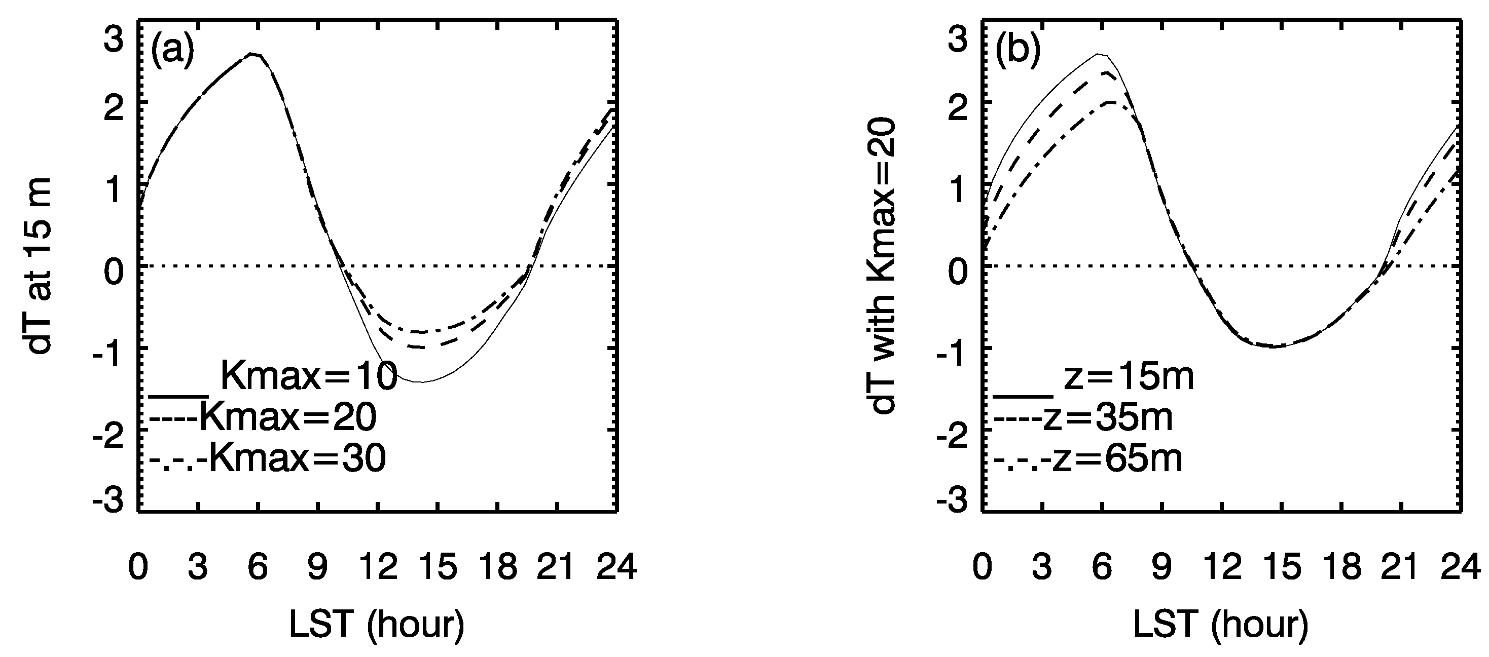
3.2. Response to the Change Of Diffusivity

The simulation results from GEM-MACH show that while the diurnal variations of diffusivity change are similar over different urban areas in winter, the change in summer are different. To compute the temperature response to the change of diffusivity, the diurnal variation of $\Delta K$ similar to that over New York city showing in Figure 5a is used. In the computation, the temperature gradient between 8:00 a.m. and 8:00 p.m. is −0.01([${}^{°}$C][m${}^{-1}$]) and is 0.02 ([${}^{°}$C][m${}^{-1}]$) between 8:00 p.m. to 8:00 a.m. below 20 m and 0 above 20 m to reflect the temperature inversion.

Figure 5b shows that positive $\Delta K$ leads to about 0.2 ${}^{°}$C temperature enhancement in the early morning and at nighttime during which gradient of reference temperature is negative. Positive/negative $\Delta K$ in winter/summer leads to very weak negative/positive temperature response during the daytime when the gradient of reference temperature is negative. Strong modulation by diffusivity can be seen in the diurnal variation of temperature response to $\Delta K$. Although the magnitude of $\Delta K$ during the daytime in summer is much stronger than $\Delta K$ in the early morning, the temperature response is much weaker suggesting a strong modulation effect by the strong diffusivity during the daytime. In the figure, −0.2 ${}^{°}$C temperature response around 7:00 p.m. in winter is attributed to weak diffusivity. The comparison between Figure 3c and Figure 5b suggests that the magnitude of the temperature response to $\Delta J_b$ is much larger than that to $\Delta K$ suggesting that $\Delta J_b$ is a major contributor to the UHI effect in the early morning.

The above numerical results show that the contribution of the change of surface heat flux to the change of temperature is dominant. The temperature response to the change of surface heat flux has a similar evolution pattern and magnitude to those in GEM-MACH simulation with the TEB scheme [10]. The evaluation of the temperature prediction by GEM-MACH against ground-based observations shows that the inclusion of the TEB scheme significantly improves the bias and root-mean-square-deviation of the temperature prediction over downtown Toronto. Therefore, the similar results of the 1-D model and numerical weather prediction model suggest that the 1-D model can describe the fundamental mechanism of diurnal variation of temperature response to the change of surface heat flux.

4. Summary

Urbanization has a great impact on urban temperature. The change of urban temperature has been studied extensively due to its impact on human comfort and safety, urban ecology and energy demand. To understand some important features of the diurnal temperature change shown in observations and 3-D numerical model simulations from GEM-MACH, a 1-D diffusion model is employed in this work to investigate the mechanism underlying the temperature responses to the change of urban surface heat flux and vertical turbulent mixing.

The solution to the linearized 1-D diffusion equation around a reference state is derived by employing the GF method. It shows that the temperature response to the change of surface heat flux is equal to the convolution of the change of heat flux and the GF. Thus the impact of the change of surface heat flux is modulated by the GF, and the temperature response at a given time t depends not only on the value of the change of surface heat flux at that time but also on the value prior to t. Since the GF is positive, enhanced/reduced urban heat flux change would lead to temperature enhancement. If the reference diffusion coefficient is only the function of time, the value of the GF is inversely proportional to the square root of the reference diffusion coefficient near the surface. Thus, GF is large when the diffusivity is weak in the early morning and at nighttime, and is small during daytime when diffusivity is strong. Consequentially, temperature response to the change of surface heat flux is significantly reduced during daytime. The modulation effect by the GF and the convolution effect explain that although the magnitude of surface flux reduction during the daytime is much larger than that in the early morning, the magnitude of the temperature response is smaller than that in the early morning.

The analytical results also show that temperature response to the change of diffusion coefficient is modulated by the vertical gradients of reference temperature and the GF. The numerical results show that if the reference diffusion coefficient depends only on time, the vertical gradient of the GF is negative under 80 m. Therefore positive diffusion coefficient difference would enhance urban temperature in the early morning when the vertical gradient of reference temperature is positive due to temperature inversion. Because the gradient of the reference temperature is negative during the daytime, reduction of the diffusion coefficient by urbanization in summer would also enhance temperature, but the enhancement would be significantly reduced by strong diffusivity. For the same reason, the magnitude of temperature reduction by the enhancement of the diffusion coefficient during the daytime in winter would also be reduced.

Temperature response to the change of surface heat flux and diffusivity are investigated numerically. The numerical results show that with the typical diurnal variations of the change of surface heat flux and diffusivity and reference variables, temperature response to the change of surface heat flux is much larger than the response to the change of diffusivity. Since the magnitude and diurnal variation pattern of temperature response in this work are quite similar to the numerical simulation results from GEM-MACH, the analytical results of this paper can be employed to interpret the 3-D GEM-MACH model simulation results.

References

1. Oke, T.R. Boundary-Layer Climate; Methuen: London, UK, 1987; 435p. [Google Scholar]
2. Oke, T.R. The Heat Island of the Urban Boundary Layer: Characteristics, Causes and Effects. In Wind Climate in Cities, NATO ASI Series (Series E: Applied Sciences); Cermak, J.E., Davenport, A.G., Plate, E.J., Viegas, D.X., Eds.; Springer: Dordrecht, The Netherlands, 1995; pp. 81–108. [Google Scholar]
3. Oke, T.R. The heat island of the urban boundary layer: Characteristics, causes and effects. In Wind Climate in Cities; Cermak, J.E., Ed.; Kluwer Academic Publisher: Dordrecht, The Netherlands, 1995; Volume 84, pp. 35–45. [Google Scholar]
4. Grimmond, C.S.B.; Roth, M.; Oke, T.R.; Au, Y.C.; Best, M.; Betts, R.; Carmichael, G.; Cleugh, H.; Dabberdt, W.; Emmanuel, R.; et al. Climate and more sustainable cities: Climate information for improved planning and management of cities (Producers/capabilities perspective). Procedia Environ. Sci. 2010, 1, 247–274. [Google Scholar] [CrossRef] [Green Version]
5. Roth, M. Urban Heat Islands. In Handbook of Environmental Fluid Dynamics; Fernando, H.J.S., Ed.; CRC Press/Taylor & Francis Group, LLC: Boca Raton, FL, USA, 2013; pp. 143–159. [Google Scholar]
6. Martilli, A. Current research and future challenges in urban mesoscale modelling. Int. J. Climatol. 2007, 27, 1909–1918. [Google Scholar] [CrossRef]
7. Masson, V. Urban surface modeling and meso-scale impact of cities. Theor. Appl. Clim. 2006, 84, 35–45. [Google Scholar] [CrossRef]
8. Leroyer, S.; Blair, S.; Mailhot, J.; Strachan, I.B. Micro-scale Numerical Prediction over Montreal with the Canadian external urban modeling system. J. Appl. Meteor. Clim. 2011, 50, 2410–2428. [Google Scholar] [CrossRef]
9. Stroud, C.A.; Ren, S.; Zhang, J.; Moran, M.D.; Akingunola, A.; Makar, P.A.; Munoz-Alpizar, R.; Leroyer, S.; Belair, S.; Sills, D.; et al. Chemical Analysis of Surface. Level Ozone Exceedances during the 2015 Pan American Games. Atmosphere 2020, 11, 572. [Google Scholar] [CrossRef]
10. Ren, S.; Stroud, C.; Belair, S.; Leroyer, S.; Munoz-Alpizar, R.; Moran, M.; Zhang, J.; Akingunola, A.; Makar, P. Impact of urbanization on the predictions of urban meteorology and pollutants over four major North American cities. Atmosphere 2020, 11, 969. [Google Scholar] [CrossRef]
11. Masson, V. A Physically-Based Scheme For The Urban Energy Budget In Atmospheric Models. Bound.-Layer Meteorol. 2000, 94, 357–397. [Google Scholar] [CrossRef]
12. Martilli, A. Numerical study of urban impact on boundary layer structure: Sensitivity to wind speed, urban morphology and rural soil moisture. J. Appl. Meteor. 2002, 41, 1247–1266. [Google Scholar] [CrossRef]
13. Oke, T.R. The energetic basis of the urban heat islan. Q. J. R. Meteorol. Soc. 1982, 108, 1–23. [Google Scholar]
14. Cleugh, H.A.; Oke, T.R. Suburban-rural energy balance comparisons in summer for Vancouver, B.C. Bound.-Layer Meteorol. 1986, 36, 351–369. [Google Scholar] [CrossRef]
15. Makar, P.A.; Gong, W.; Hogrefe, C.; Zhang, Y.; Curci, G.; Žabkar, R.; Milbr, T.J.; Im, U.; Balzarini, A.; Baró, R.; et al. Feedbacks between air pollution and weather, Part 1: Effects on weather. Atmos. Environ. 2015, 115, 442–469. [Google Scholar] [CrossRef]
16. Leij, F.J.; Priesack, E.; Schaap, M.G. Solute transport modeled with Green’s functions with application to persistent solute source. J. Contam. Hydrol. 2000, 41, 155–173. [Google Scholar] [CrossRef]
17. Jaiswal, D.K.; Kumar, A.; Yadav, P.R. Analytical solution to the one-dimensional advection-diffusion equation with temporally dependent coefficients. J. Water Resour. Prot. 2011, 3, 76–84. [Google Scholar] [CrossRef] [Green Version]
18. Chen, J.S.; Liu, C.W. Generalized analytical solution for advection-dispersion equation in finite spatial domain with arbitrary time-dependent inlet boundary condition. Hydrol. Earth Syst. Sci. 2011, 15, 2471–2479. [Google Scholar] [CrossRef] [Green Version]
19. Holzer, M.; Hall, T.M. Transit-Time and Tracer-Age Distributions in Geophysical Flows. J. Atmos. Sci. 2000, 57, 3539–3558. [Google Scholar] [CrossRef] [Green Version]
20. Chen, B.; Chen, J.M.; Liu, J.; Chan, D.; Higuchi, K.; Shashkov, A. A vertical diffusion scheme to estimate the atmospheric rectifier effect. J. Geophys. Res. 2004, 109, D04306. [Google Scholar] [CrossRef]
21. Arson, V.E.; Volkmer, H. An idealized model of the one-dimensional carbon dioxide rectifier effect. Tellus 2008, 60B, 76–84. [Google Scholar]
22. Ren, S. Solutions to the 3-D transport equation and 1-D diffusion equation for passive tracers in the atmospheric boundary layer and their applications. J. Atmos. Sci. 2019, 76, 2143–2169. [Google Scholar] [CrossRef]
23. Kevin, D.C.; Beck, J.V.; Haji-Sheikh, A.; Litkouhi, B. Heat Conduction Using GREEN’S Functions; CRC Press, Taylor Francis Group: Boca Raton, FL, USA, 2011; 663p. [Google Scholar]
24. Bateman, H. Tables of Integral Transforms; McGraw-Hill Book Company, Inc.: New York, NY, USA, 1954; Volume 1, 391p. [Google Scholar]
Figure 1. Distribution of G ˜ 1 d / z on the z z plane with K t = 1 and a wide range of T . Contours with a positive value are shaded.
Atmosphere 11 00978 g001
Figure 2. Same as Figure 1 but with K t = 5 .
Atmosphere 11 00978 g002
Figure 3. Diurnal variation of Δ J (a), reference diffusion coefficient (b) and diurnal temperature response to Δ J at 15 m (c) in the summer case (solid lines) and winter case (dashed lines).
Atmosphere 11 00978 g003
Figure 4. Diurnal variation of temperature response to Δ J at 15 m with different K t , m a x (a) and at different height with K t , m a x = 20 (b).
Atmosphere 11 00978 g004
Figure 5. Diurnal variation of Δ K (a), and diurnal temperature response to Δ K t at 15 m (b) in the summer case (solid lines) and winter case (dashed lines).
Atmosphere 11 00978 g005