Towards a Better Design of Convection-Allowing Ensembles for Precipitation Forecasts over Ensenada, Baja California, Mexico

Abstract

Convective ensembles promise to increase forecast accuracy while at the same time providing information on the probability of the forecast. A vast number of different methods of ensemble creation have been developed over time. Here, initial conditions and model error uncertainties are represented by a convective-allowing ensemble with more than 50 members. The results are analyzed using one case study with relatively high precipitation over Ensenada, Baja California, Mexico. The ensemble members are perturbed using random initial perturbations, breeding, and the Stochastic Kinetic Energy Backscatter parameterization (SKEBS) within the Weather Research and Forecasting (WRF) model. The aim is to improve the high-resolution ensemble design provided in a previous study for the same region by maximizing the spread of an ensemble with low member count. To this end, a comparative analysis of the members is performed using perturbation growth rates and information entropy. In addition, a comparative verification is performed using observations from one automatic meteorological station and satellite-derived precipitation data. It was found that the growth rates and the one-dimensional power spectral density of the initial perturbation fields are clustered depending on each member’s origin and the methods used to generate the breeding members. An inverse relationship was observed between these two variables, which can be useful for selecting appropriate initial condition perturbations. The dynamical injections of energy, introduced as perturbations to the numerical fields by the SKEBS method, were essential to maintain positive growth rates during the simulation period. Evaluation of the information entropy suggests that a selection of a set of members generated by the SKEBS method is best for increasing the ensemble spread while saving computer resources.

1. Introduction

Convection-allowing ensemble systems are increasingly used for weather forecasting in various applications [1,2,3,4,5,6,7]. These ensembles are a composition of multiple, different realizations (members) of the atmospheric dynamical state. The aim of performing these ensemble runs is to provide a more representative distribution of the initial and boundary conditions, and model errors to reduce forecast uncertainties. Furthermore, their high spatial resolutions, 4 km or less, represent the convective regime more realistically at a local scale, improving the accuracy of, for example, quantitative precipitation forecasts [8,9].

The inaccuracy and lack of resolution of the initial meteorological data motivate the use of perturbations to the initial and boundary conditions in a high-resolution ensemble. The numerical forecasts of coarser-resolutions used to drive limited-area models are another source of error. Different methodologies have been applied to construct perturbations, such as the addition of random perturbations [10], breeding [11,12], and singular vectors [13]. On the other hand, uncertainty due to model errors is commonly addressed through multimodel [14] or multiphysics [15] ensembles. Recently, the introduction of time and spatially-correlated stochastic perturbations during model integration have shown to improve the ensemble spread [16,17,18,19,20,21]. Du et al. [22] provide a vast list of methodologies to create ensemble forecasts.

A wide range of studies provide information on the performance of each of the above methods regarding the representation of the probability distribution function of the atmospheric state. For example, Toth and Kalnay [12] made a comprehensive analysis of the use of the breeding vectors in global ensemble forecasts. As they highlighted, the advantages of using this method over singular vectors and random initial perturbations include its simplicity, low computational costs, and a good representation of the spatial structure of the analysis errors. However, they also stated that using different perturbation techniques may contribute to the success of ensemble forecasts. Similarly, after comparing various initial condition perturbation strategies, Bowler [23] determined that the random perturbations methodology is, at least, as good as any other. Magnusson et al. [24] performed a comparative study between various initial perturbation strategies focusing on the perturbations’ growth. It showed that perturbations need to be located on the attractor to start growing steadily at short time scales.

Greybush et al. [25] analyzed several sets of ensemble forecasts at high-resolution using initial condition perturbations, stochastic perturbations of dynamical and physical fields at runtime, and multiphysics strategies for one winter case study. They showed that all methods improved scores relative to the control run. Nevertheless, the multiphysics method scored best for reliability concerning precipitation observations. Li et al. [26] used model error representation methods to investigate whether stochastic parameterization schemes could outperform multiphysics schemes. They found that the multiphysics ensemble method performed better than the stochastic schemes. However, results could vary depending on the physics included in the model, and the domain resolution [20,27,28].

Méndez-Turrubiates et al. [29] explored the feasibility of quantitative precipitation predictions through high-resolution ensemble forecasts based on the Weather Research and Forecasting (WRF) model. Their implementation was the first implementation of a convective-allowing ensemble over Ensenada, Baja California, Mexico. However, the authors focused on post-processing techniques to improve precipitation-related forecast skill scores while applying only random perturbations to the initial conditions using a generic, low-resolution background error covariance matrix. Therefore, those perturbations were characterized by large decorrelation scales and smaller increments [30]. However, the shortening of the spatial perturbation structures’ length scales could add value to the underlying atmospheric dynamics [31].

The present investigation extends Méndez-Turrubiates et al.’s work [29] with a focus on applying different perturbation techniques to represent initial conditions and model error uncertainties. The general intent is to evaluate the performance of a high-resolution ensemble system designed to maximize the spread with the least set of members possible and improve precipitation forecasts. The approach uses three distinct types of ensemble members: (1) random perturbations to the initial conditions, (2) perturbations through the breeding method, and (3) model error representation through the Stochastic Kinetic Energy Backscatter parameterization. More than 50 members are analyzed within a convective-allowing ensemble for one case study of relatively intense precipitation over the region of interest.

In Section 2, we first describe the data, the case study location and date, and the methods. Then, we present the analysis of the perturbations provided by the various strategies. In Section 3, the initial perturbations are characterized in terms of the average spectral energy, which correlates with their initial growth rates. It is shown that the evolution of those growth rates can describe the member’s behavior in time and has implications for the ensemble spread. An entropy-based analysis was performed, and it will be shown how this can be used to determine the type of perturbations that maximizes the amount of new information provided by each ensemble member. Verification of the individual ensemble members against observations is also provided.

2. Data and Methods

The spatial and temporal coverage of the case study is introduced in Section 2.1, followed by the three data sources that are used in this study: model data to initialize the model, site observations for evaluation, and remotely sensed precipitation data, which enables the verification across the whole domain. These sources are detailed in Section 2.2 and Section 2.3 below. Then the ensemble member configuration is presented (Section 2.4), followed by the details of the configuration of the WRF model (Section 2.5) and the generation of perturbations (Section 2.6). The manuscript continues by presenting the analysis methods used to evaluate the ensemble members (Section 2.7), followed by the forecast verification metrics used (Section 2.8).

2.1. Spatial and Temporal Coverage of the Case Study

In Figure 1, the white-edged square encloses the study area. As one can see, it comprises most of the southwestern USA (California and Arizona) and the northern part of the Peninsula of Baja California, Mexico. Westward is the Pacific Ocean. The northern part of the Gulf of California appears in the bottom-right corner of the Figure. Particular attention will be given to the area in the center of the spatial domain, where most precipitation occurred during our present case study. The study area was centered over the Port of Ensenada. The black star marker in Figure 1 represents the location of the Lopez Zamora automatic meteorological station. Observations from this station wer gatheered for the case study. Such observations covered 48 h, starting on 27 February 2017 (20170227) at 00 UTC. This date was selected because the highest amount of precipitations for the year 2017 was reported during February 27 and 28, as a result of the movement of a cold front.

2.2. Initial and Boundary Conditions of the WRF Model

The initial and boundary conditions were extracted from the North American Mesoscale Forecast System (NAM) forecasts [32], provided by the National Centers for Environmental Prediction (NCEP). NAM products have various coverage and spatial resolutions. Here we used the inner grid of the NAM model (NAM05) covering the United States of America (USA) and most of Canada and Mexico with a spatial resolution close to 5 km. NAM05 provides outputs in Grib 2 format every day as a result of one initialization at 00 UTC producing valid forecasts every 1–3 h and up to 60 h each run. Therefore, its time and spatial coverage satisfy the boundary and initial conditions of the ensemble implementation described within the next sections.

2.3. Observational Data at the Meteorological Station and Imerg

Figure 2 shows time series plots for data collected at the Lopez Zamora (ZMS) station maintained by the National Meteorological Service of Mexico (SMN). Data for precipitation (RAIN) in mm/h, temperature (T) in degree Celsius, water vapor mixing ratio (QVAPOR) in g/kg, and surface pressure (P) in hPa, were used.

Most of the precipitation occurred after 12 UTC of 27 February 2017. After hour 32 in Figure 2, which corresponded to 08 UTC of 28 February 2017, the dry air mass following the cold front sets in with relatively high pressures and no precipitation. The minimum temperature of around 10 degree Celsius, reached at 14 UTC of 28 February 2017 (Hour 39), could also have been related to heat loss during the nighttime hours.

NASA Global Precipitation Measurement (GPM) Integrated Multi-satellite retrievals for GPM (IMERG) [33] precipitation data inter-calibrates, merges, and interpolates satellite microwave precipitation estimates, together with microwave-calibrated infrared satellite estimates, and precipitation gauge analyses, to form a spatio-temporal dataset. The IMERG product used here was the 3IMERGHH product, which provides precipitation estimates every 30 min at a spatial resolution of 0.1${}^{\circ }$, corresponding to ∼11 km. We integrated the precipitation data into hourly estimates without modifying the product’s spatial resolution. Figure 3 shows the hourly precipitation data for the study area, corresponding to 19 UTC of 27 February 2017, when the ZMS reported the most intense precipitation.

2.4. Ensemble Members Design

The high-resolution ensemble had 56 members, corresponding to 55 perturbations and a control run. As discussed before, the numerical simulations for each ensemble member started at 00 UTC of 27 February 2017 and ended 48 h later. The outputs were stored with a frequency of 1 h during the study period.

Table 1. Labeling used to identify each ensemble member. The color represents the source of the members’ perturbation: control (black), control with  [29] setup (cyan), CV3 covariance matrix (yellow), CV7 covariance matrix (orange), SKEBS (lavender), breeding (carnation pink), and breeding unsigned from SKEBS (rhodamine).

Cu00u	Op71u	Op73u	Su01u	Su05u	Bn31n	Bn71n	Bn72n	Bn73n	Bn74n	Bn01u	Bn05u
Cu09u	On71u	On73u	Su02u	Su06u	Bp31n	Bp71n	Bp72n	Bp73n	Bp74n	Bp01u	Bp05u
Op31u	Op72u	Op74u	Su03u	Su07u	Bn31p	Bn71p	Bn72p	Bn73p	Bn74p	Bn02u	Bn06u
On31u	On72u	On74u	Su04u	Su08u	Bp31p	Bp71p	Bp72p	Bp73p	Bp74p	Bp02u	Bp06u
										Bn03u	Bn07u
										Bp03u	Bp07u
										Bn04u	Bn08u
										Bp04u	Bp08u

shows the label and color of each ensemble member. The color depended on the source of the members’ perturbation. The color scheme assigned to the members was the same throughout the paper.

The labeling provided the following information about the member. The first letter indicates the source of the perturbation used to produce the member. Four choices may appear:

• C: control run,
• O: random initial perturbations using RANDOMCV from WRF Data Assimilation (WRFDA),
• B: initial conditions perturbed using the breeding technique [12], or
• S: using the Stochastic Kinetic Energy Backscatter Scheme (SKEBS).

Note that a second member using the C letter is shown in the Table, Cu09u, representing another deterministic run of the WRF model using a different set of physical parameterizations.

The second letter indicates the sign of the perturbation, which can be positive (p), negative (n), or does not apply (u). The perturbation sign refers to whether it was added to (p) or subtracted from (n) the unperturbed initial conditions. Hence, signed members appeared in pairs, which are symmetric to the unmodified initial conditions to improve the coverage of the associated uncertainties [12]. Unsigned members, corresponding to SKEBS members and the control run, were those to which the signed pairing could not be applied due to the nature of the perturbation method.

The second letter was followed by two digits used to differentiate between random perturbation methods or track the breeding members’ heritage. More information about these methods is given below in Section 2.6.

The third and final letter indicats the sign of the perturbation from which the current one originated. Note that only breeding members were allowed to inherit the previous sign, and it did not apply for the other members.

2.5. Set-Up of the WRF Model

The WRF model version 3.9 was used here [34]. The numerical domain, labeled D01, is shown in Figure 1. The model grid had a spatial resolution of 3 km.

Table 2. Dynamical and physical parameterizations used.

Parameterizations	Selection	Comments	References
cumulus (cu)	None (cu = 0)	convection solved explicitly at current resolution	[35,36]
microphysics (mp)	Thompson (mp = 8)	Best scheme at high resolution for this region	[37,38]
planetary boundary layer (pbl)	Yonsei University scheme (pbl = 1)	lower bias with respect to observations	[38,39], [40]
long (lw) and short (sw) wave radiation	Rapid Radiative Transfer model (RRTMG) (sw = 4, lw = 4)	represent sub-grid scale radiative processes	[41]
surface layer (sfc)	MM5 model revised scheme based on Monin-Obukhiv (sfc = 1)	compatible with pbl	[42,43]
diffusion option (diff_opt)	full diffusion (diff_opt = 2)	acurately compute horizontal gradients in sloped coordinates	[34]

summarizes the dynamic and physical parameterizations used. The WRF preprocessing system (WPS) selected default topography and soil information with a resolution of 30 s, corresponding to ∼1 km. This resolution was sufficient to describe the dynamics, together with flux exchange processes at the resolving scale; see also Figure 1.

We applied Digital Filtering Initialization (DFI) to the simulations to reduce the model spin-up time. In this case, we used the recommended Dolph filter [44], a low-pass digital time filter that minimizes the maximum difference between a filter’s transfer function and an ideal transfer function in the pass and stop bands. The scheme applies the filter twice: first in an adiabatic backward integration, and then in a forward diabatic integration [34].

The deterministic realization Cu09u (cyan in Table 1) was introduced as a member of the ensemble using a different set of physical parameterizations. The goal was to establish comparisons with the control run (Cu00u) and evaluate the sensitivity to changes in the physics configuration (multiphysics ensemble). This member followed the experiment design implemented by Méndez-Turrubiates et al. [29], where the outer domain had a spatial resolution of 4 km. In addition, it used the Kain–Fritsch cumulus parameterization [45], combined with the WSM3 microphysical scheme [46].

2.6. Ensemble-Member Perturbation Methods

Besides the control run (Cu00u) and the unperturbed alternative-physics member (Cu09u), for which descriptions have been provided above, three other perturbation methods were used in this research to generate the ensemble: random perturbations, Stochastic Kinetic Energy Backscatter, and breeding. Each of these methods will now be discussed in turn.

2.6.1. Random Perturbations

The first method used the RANDOMCV routine from the WRF Data Assimilation (WRFDA) module. This routine used a background error covariance matrix to generate the members’ new initial and boundary conditions (IBC). The latter was accomplished by adding seeded random perturbations to the unmodified IBC from NAM. Each of these, hereafter called positive members (Op31u, Op71u, Op72u, Op73u, and Op74u), also produced a negative member (labeled On31u, On71u, On72u, On73u, and On74u, respectively), by subtracting twice the randomly generated perturbation from its corresponding positive member. Toth and Kalnay [12] used this technique to generate symmetric breeding perturbations, and we expanded this idea to random perturbations to better account for the uncertainties in the IBC. This way, a total of 10 different members were generated from random perturbations of the IBC. Only the initial boundary conditions were updated after the perturbation was applied. The boundary conditions provided by the NAM coarser-resolution numerical forecasts were not modified.

The main differences between the positive members are discussed next. The member Op31u, and by extension its negative pair (On31u), were created using the CV3 covariance matrix provided within the WRF model package, obtained from a global model simulation with a low spatial resolution [34]. Within these members, we preserved the typical length scale and variances of the errors described by the CV3; see yellow members in Table 1. This method was used to generate random perturbations in [29]. The remaining positive, randomly perturbed members (Op71u, Op72u, Op73u, Op74u) were produced using the domain-specific CV7 covariance matrix generated by the WRF model for the first 6 months of the year 2017. CV7 was created with the GEN_BE tool [47], provided within WRFDA, using the NMC (National Meteorological Center) method [48]. It is worth noting that these four members differed not only in the seed used to generate the perturbations but also in the length scale of the background error covariance matrix, while Op71u preserved the length scale of CV7, Op72u, Op73u, and Op74u used half, three-halves, and twice the length scale of the typical background errors, respectively. The typical decorrelation scales in the CV3 randomly perturbed fields were around three times larger than those of the CV7. These members and their negative pairs are highlighted in orange in Table 1.

2.6.2. Stochastic Kinetic Energy Backscatter

A total of eight members were generated using the Stochastic Kinetic Energy Backscatter Scheme (SKEBS) provided within the WRF model. SKEBS acts on the wind rotational, and the potential temperature tendencies in the WRF simulations by adding stochastic, vertically-barotropic perturbations at run time. It works on the basis that the model does not correctly represent the turbulent kinetic energy flux onto the subgrid scales. In turn, the model truncation errors, for example, are projected as kinetic energy at the model grid scales [17,49]. The parameters set to produce the stochastic perturbations followed [19]. With a backscatter rate of ${10}^{-5}$ for the stream function and ${10}^{-6}$ for the temperature, and a decorrelation time of three hours, they analyzed model errors in a convection-permitting ensemble system with a similar spatial resolution in their outer numerical domain. In addition, the difference between the SKEBS members (marked green in Table 1) is the seed used to generate their perturbations. From a practical point of view, the main difference between this method and the others was that perturbations were dynamically introduced during the simulation period.

2.6.3. Breeding

The rest of the members in our convection-allowing ensemble study were produced using the breeding method [12] and setting the breeding cycle to 24 h. Therefore, simulations were performed for the day before 27 February 2017 at 00 UTC using the members generated by both methods mentioned above. It can be seen in Table 1, that each of those members produced two new breeding members, 36 in total, highlighted in pink. For example, the member Op31u run for the day before (20170226 at 00UTC) bred two symmetrical members, Bp31p and Bn31p. The energy conservation criteria based on the root-mean-square equation were used as the norm to rescale the perturbations generated with this method [12]. As in the case of random perturbations, the breeding method only affected the initial boundary conditions when the perturbations were added to the initial fields.

2.7. Methods for Perturbations Analysis

The two methods used to analyze the state differences in all members are presented below. One was based on the Lyapunov exponent and the other on Information Entropy (IE). The state differences, conceived as the difference between each member and the control run (Cu00u) fields, were analyzed for the variables T, QVAPOR, P, wind speed (WSP), and RAIN whenever possible. As these differences were computed at every hour during the study period, we linked to each member three stages of its corresponding perturbation. The initial perturbation was the one generated by either method described above. It was used to start the simulation of that member. We also used the term initial perturbation after DFI, to identify the perturbation at the beginning of the simulation but after carrying out the Digital Filter Initialization process within WRF. At any forecast hour of the simulation period after 27 February 2017 at 00 UTC, we named it only by member perturbation.

2.7.1. Lyapunov Exponent Method

We used the Lyapunov exponent to analyze the exponential growth rate of the evolving perturbations. In a chaotic system, as the WRF governing equations [50,51], the perturbations grew in time exponentially. At time $∆t$, the exponential growth of the perturbation $∆P$ was determined by the factor $\lambda$ following Equation (1), also called the Lyapunov exponent. In this equation, $∆P_0$ represents the same perturbation at the initial state. Even in a chaotic system, $\lambda$ can vary throughout the attractor. However, as $∆t$ goes to infinity, the dominant Lyapunov exponent is reached, and wherever it is greater than zero, there is chaos [24].

$$\lambda =\frac{1}{∆t}ln(\frac{\parallel ∆P\parallel }{\parallel ∆P_0\parallel })$$

(1)

2.7.2. Information Entropy Method

The analysis of Information Entropy (IE) determines the uncertainty or amount of new information each member provides to the ensemble [52]. Theoretically, all the ensemble members should provide the same amount of new information to maximize the entropy of the ensemble probability distribution [53]. Ma et al. [54] used this method to analyze the perturbation information amount in breeding-based convection-allowing ensembles quantitatively. The information entropy was computed with Equation (2) at any given point in time and space. $\mathbf{P}=[∆P_1,∆P_2,\dots ,∆P_N]$ represents the set of perturbations contained by the N members of the ensemble. The operand $K_{PDF}[\ast ]$ is the discrete probability density function of $\mathbf{P}$, estimated from a Gaussian kernel with the Silverman method [55].

$$IE=-{\int }_N{K}_{PDF}\left[\mathbf{P}\right]\ast {log}_2\left(K_{PDF}\left[\mathbf{P}\right]\right)d\mathbf{P}$$

(2)

2.8. Verification Metrics

The grid-to-point and grid-to-grid verification methods were used in this research. The former was applied to assess the WRF ensemble outputs using the Lopez Zamora meteorological station. The latter was used to verify the ensemble precipitation with IMERG data. Since we were analyzing only one case study, and because observations for this region were scarce, the primary purpose of the verification analysis was to compare the relative performance between the ensemble members and to assess the possibility of improving the ensemble results.

Seven statistical metrics were used: bias, mean, standard deviation, correlation, root mean square error, probability of detection (POD), and false alarm ratio (FAR) [56]. Bias was used to compare the ensemble members and was computed as the average of any field difference. The mean or average of a variable, F, in time or space, is computed as follows:

$$\overline{F}=\frac{1}{N}\sum _{i=1}^N{F}_i,$$

where N is the number of elements of the variable in the dimension(s) being averaged. The standard deviation (STD) measured the ensemble’s spread when computed using the members as the ensemble dimension. This metric was calculated as

$$ST{D}_F=\sqrt{\frac{{\displaystyle \sum _{i=1}^N}{(F_i-\overline{F})}^2}{N-1}}.$$

Pearson’s linear correlation coefficient (COR) determined the linear relationship between observations and forecasts:

$$COR=\frac{{\displaystyle \sum _{i=1}^N}{F}_i{O}_i-N\overline{F}\overline{O}}{(N-1)ST{D}_{F}ST{D}_O}.$$

The root-mean-square error (RMSE),

$$RMSE=\sqrt{\frac{1}{N}\sum _{i=1}^N{(F_i-O_i)}^2},$$

measured the error of the forecast, F, with respect to the observations, O, with zero value indicating a perfect forecast. Similarly, if we let N be the ensemble dimension, the ensemble error could be determined.

The dichotomic statistic metrics, POD and FAR, were used to compare the forecasts with IMERG precipitation data. Their formulas are presented below, where the dichotomic variables, a, b, c, and d, were determined using the contingency table (see

Table 3. Contingency table.

	Observations
Forecast	Yes	No
Yes	a (hits)	b (false alarms)
No	c (misses)	d (correct rejections)

). This table counts the hits, misses, false alarms, and correct rejections of a prediction instance of an event relative to its observation at a given point. A precipitation event occurred for rainfall values equal to and higher than 0.1 mm/h.

$$POD=\frac{a}{a+c};$$

$$FAR=\frac{b}{b+d}$$

3. Results and Discussion

The performance of the different perturbation strategies was analyzed in three stages. The first stage, Section 3.1, analyzes the perturbations, their growth rates, and information entropy. This stage provides information on which member will add the most value to the final ensemble. Then, in the second stage, Section 3.2, the individual members and the full ensemble are compared to the observations. Finally, in Section 3.3, an ensemble is created from a subset of the members and its ensemble forecast compared to the observations. This final comparison then proves the manuscript’s hypothesis that members can be selected a priori to form a more skillful ensemble.

3.1. Analysis of Initial Perturbations and Perturbation Growth

The results presented below describe the initial perturbations used in the ensemble. The perturbation growth and information entropy evolution are analyzed to find the optimal set of members that maximizes the ensemble spread.

3.1.1. The Growth Rate of The Perturbations

In Figure 4, we show the spatially-averaged growth rate of the perturbations for each member, computed for every hour (thick colored lines), using Equation (1). The shading areas represent the vertical variability of the growth rates. It can be noted that the growth rate of the perturbations decreased rapidly during the first 6 hours for most simulations. In this respect, it is understood that numerical imbalances in the perturbed initial conditions could produce gravity wave motions that decreased the amplitude of the perturbations in the first hours of the forecast simulation. Sound waves also helped to propagate the energy associated with the perturbations in high-resolution atmospheric domains [57].

The breeding members coming from CV3 perturbations (light pink) showed different behavior. Their growth rate was never positive but increased in the first 6 hours, as they were initially more negative. These members possessed the lowest growth rate values at all times. All members reached a steady growth rate towards the end of the simulation period, as expected [24]. Magnusson et al. [24] also noted that the error was supposed to grow exponentially during the first hours of an atmospheric model integration while the growth rate decreased. After a while, long enough to consider it infinite, the error saturated, and so the growth rate stabilized as Equation (1) converged to the dominant Lyapunov exponent.

The members appeared grouped depending on the source and method with which the initial perturbation fields were created. Firstly, SKEBS simulations (green) showed the highest growth rates, which remained positive throughout the simulation. The member with different physics (Cu09u in cyan) exerted a similar behavior but with lower initial growth values. Meanwhile, the breeding members coming from SKEBS perturbations (dark pink) showed positive growth at first but ended up with negative average growth rates, closer to zero (no growth). Finally, randomly-perturbed (orange) and breeding members (pink) from CV7 behaved alike: initially-positive growth rates rapidly became negative with values around −0.1. The members with randomly-perturbed initial fields using CV3 (yellow) always had negative growth rates below that value. These results are in contrast with [24], who found that for 5000 simulation cases, the average growth rate would be around unity for these kinds of members using the chaotic model from [50], although the governing equations in WRF used to simulate our case study represent a chaotic system for which positive Lyapunov exponents are expected. Figure 4, on the other hand, presents results averaged in physical space.

Figure 4 shows the effectiveness of the SKEBS parameterizations in WRF to simulate the perturbation growth behavior with a different physics configuration without the need to change the model physics. The continuous injections of perturbations to the wind and temperature fields made the all-time positive growth rate possible. Even so, those growth rates were low (<0.2), while perturbations from breeding and randomly-perturbed members decreased on average toward the end of the simulation period. In this respect, it was probably the length scale of the integration period that made the initial condition perturbation methods unable to produce growing perturbations. For longer forecast periods, even random perturbations are expected to grow after reaching the attractor [24].

For short-range forecasts, however, high, positive initial growth rates are essential to ensure positive growth rates throughout the simulation. With that in mind, in Figure 5, the one-dimensional power spectral density (PSD) was computed for the initial perturbation fields of P, T, $Qv$, and $WSP$ near the surface. Following [58], the one-dimensional PSD of each ensemble member was obtained as the average of the two-dimensional Fourier coefficients over annuli in wavenumber space. In this Figure, all members showed the same behavior: a decreasing PSD with length scale, in agreement with [58]. However, here the members differed in terms of the overall PSD (i.e., the PSD integrated over all length scales) partly because here the data were not detrended. Kühnlein et al. [58] expected that the total spectral energy of the initial temperature perturbations to peak at around 3 km height, decreasing with altitude and toward the surface due to the filtering process of the initial conditions. All members in Figure 5b may have exceeded the values reported in the mentioned study by a few orders of magnitude.

Clustering can be observed similarly as in Figure 4. Note that members using CV3 random perturbations (yellow) had more overall PSD than those using CV7 (orange) or SKEBS (green). Breeding members (pink), on the other hand, broke into three groups responding more to the method they inherited. For example, the members with more overall PSD were the breeding perturbations coming from CV3 randomly-perturbed fields (light pink). Those related to SKEBS (dark pink) tended to have less energy associated. No special filter was applied to the initial conditions near the surface as in [58], and it was speculated that the DFI process and the conservation energy method used to obtain the breeding members influenced this outcome.

A relation can be established between results from Figure 4 and Figure 5. Generally, the members with higher overall PSD at the beginning of the simulation had lower initial growth rates. This inverse relationship was stronger for P and $WSP$, but it could also be observed for the temperature and water vapor mixing ratio. The differences in the initial growth rate between the groups could be related with three factors: (1) the degree of numerical balance among the perturbed variables throughout the entire spatial domain, (2) the degree of amplification the perturbations, randomly or not, produced on the local instabilities within the atmospheric flow and (3) the role played by the DFI process. In this regard, it can be noted that the breeding members coming from CV3 perturbations were the only simulations that did not use DFI, which happened to show an initial transient growth [59]. In addition, Ref. [57] mentioned that the moist convective instability and forced convection locally present in the simulation domain were necessary for perturbation growth.

Since results in Figure 4 are averaged in horizontal space, Figure 6 displays the vertically and time-averaged growth rate for some ensemble members. Here, the member with different physics (Cu09u, Figure 6a) had positive growth rates throughout almost the entire domain. However, the higher values appeared over the Pacific Ocean and on the northern Gulf of California. This behavior might be associated with thermal and dynamic instabilities generated as a response to the differences between this member’s and the control’s physic parameterizations. Members using SKEBS (Figure 6d,e) also had positive values but showed no definite pattern of the growth rate fields because their perturbations were randomly computed. All members had different patterns in the growth rate average field without any preferred location for their extrema. For its part, randomly-perturbed members using CV3 (e.g., Figure 6b) presented negative growth, and their breeding counterparts (Figure 6f for the given case) showed even lower values. The randomly-perturbed members using CV7 and associated breeding members (Figure 6c,g) showed areas of positive growth rates over land, and even more so, the breeding members coming from SKEBS simulations (see Figure 6h,i). The latter implies that these breeding members could still be useful in an ensemble prediction system because their perturbation growth over areas of interest might have increased its spread. The localized, positive growth rates in Figure 6c,g–i were associated with the convective instability that characterized this case study.

Above we illustrated that the method used to create each member’s initial condition perturbation defined the starting value of the average perturbation growth rate. However, its effect decayed rapidly during the simulation time as the error grew. After approximately 6 hours, the boundary conditions constrained the perturbation growth from the outside. At this point, only localized growth could be found in areas with thermodynamic instability in random and breeding members, which were associated with either small scale convection due to heating and moisture sources or large scale motions such as a cold front. Therefore, spatially averaged growth rates were bound to decrease substantially with time during the simulation period. Consequently, the desired spread between the ensemble members might not have been obtained. It was observed that the 1-dimensional spectral signature of the initial perturbations could provide information regarding the initial growth rate since smaller total spectral energies were linked to higher average initial growth rates of the perturbations. In addition, it was not enough to provide suitable initial perturbations; the entire domain, including its boundaries, must be perturbed periodically to avoid growth decay. The SKEBS method met both of these requirements.

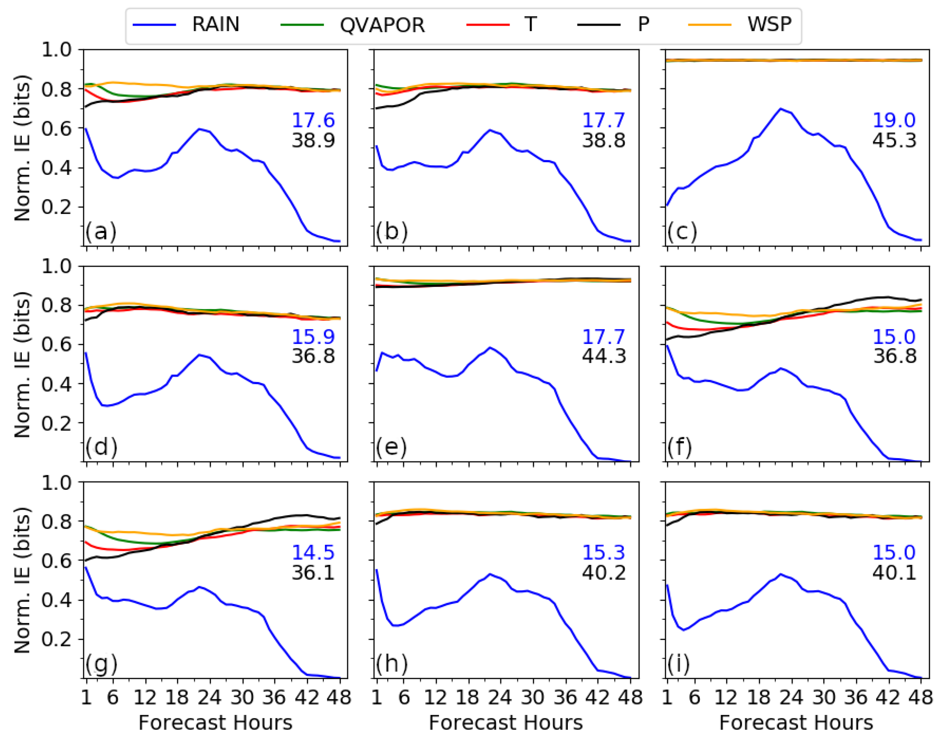
3.1.2. Information Entropy

The amount of useful information the ensemble has according to its members, the information entropy (IE), Equation (2), is plotted in Figure 7, normalized with the maximum theoretical value of this ensemble. A value of one would indicate that all members contributed equally to the ensemble, i.e., each member provides the same amount of useful information. A value of zero indicated that only one member was sufficient to describe the meteorological conditions because the model was certain about the outcome. The evolution of the spatially-averaged IE appears in Figure 7a, while the time-averaged IE is shown in Figure 7b,f, for all five meteorological variables analyzed in this study.

All continuous variables, $Qv$, T, P, and $WSP$, showed similar behavior. However, some disagreement occurred at the start of the simulation, which was related to differences in the initial perturbation fields. In addition, it should be noted that the IE values were below 0.8, indicating that some members provided more information than others. Discrete values on the domain grid points could reach up to 0.85. The maximum entropy values of these variables reflected the uncertainties in the prediction of the meteorological conditions. In addition, the content of water vapor over the northern Gulf of California and adjacent areas seemed to be the variable with the largest uncertainty. The regional variability of near-surface temperature and wind between different ensemble members may have contributde to a discrepancy between the actual amount of vapor from the Gulf of California into the atmosphere, and the amount the model “saw”.

Rain, as a discrete variable, showed a different IE evolution. In this case, it seemed to respond better to the likelihood of precipitation in a specific area. In Figure 7b, higher uncertainties were produced in the same area where precipitation would occur, in association with the cold front featuring in the case study. The white area in the lower right of the domain indicates zero IE. Here all members agreed that no precipitation would occur during the forecast period. Figure 7a shows that IE went down to zero because precipitation diminished in the whole domain towards the end of the forecast period. These results confirmed that precipitation was a difficult variable to predict. Even when it was likely to occur in one region associated with strong meteorological forcing, its intensity was highly variable at a high temporal and spatial resolution. Furthermore, relatively low IE values during rainfall hours indicated redundant information among all the ensemble members considered. Hence, a selection of these members was expected to improve IE results and the ensemble spread, while saving computer resources and time.

Table 4. Description of the experiments to evaluate the information entropy.

Name	Description	Members *
Exp1	Only positive members considered	Cu09ur, Su…, Op…, Bp…
Exp2	Only negative members considered	Cu09ur, Su…, On…, Bn…
Exp3	Only members with positive growth	Cu09ur, Su…
Exp4	Members with positive growth and breeding	Cu09ur, Su…, Bp…, Bn…
Exp5	Only negative growth considered	Op…, On…
Exp6	Members with negative growth and breeding	Op…, On…, Bp…, Bn…
Exp7	Twice the number of members with negative growth and breeding	2*(Op…, On…, Bp…, Bn…)
Exp8	Use only SKEBS and positive breeding members	Su…, Bp…
Exp9	Use only SKEBS and negative breeding members	Su…, Bn…

* See Table 2 for more information regarding the members’ name.

shows the results for nine experiments (Exp) that were performed with the methodology above. The information entropy was computed using different groups of members depending, for example, on the results described in Figure 4, and on the sign of the perturbations. Thus, for experiment one (Exp1), only positive members were considered regardless of how the perturbations were obtained. Experiment two (Exp2) used negative members. Note, however, that unsigned members like Cu09u and SKEBS (Su…) were used in the experiment using positive perturbation members (Exp1) and in the experiment using negative perturbation members (Exp2) as well.

We also tested simulations with positive growth rates (Exp 3) alone, and with breeding members (Exp4). Negative growth simulations with (Exp6) and without (Exp5) breeding were also analyzed. We studied the sensitivity of the IE calculations to the number of members and repeated information through Exp7, and analyzed the behavior of SKEBS simulations combined with positive (Exp8) and negative (Exp9) breeding members.

Figure 8 shows the evolution of IE calculations, like Figure 7a, but for all nine tests. The two values shown inside the frame of each plot represent the integral IE for the rain variable (blue), and the highest integral IE found for the rest of the meteorological variables (black); these two variables showed a similar IE evolution. Integral IE was taken as the integral over time of each meteorological variable’s hourly entropy values. The results showed that the perturbations’ sign had little influence on the IE profile and integral values; see Figure 8a,b,h,i. Both pairs of plots showed similar patterns, and the overall values were practically unaffected. The main difference between experiments Exp6 and Exp7 was the number of members. Exp7 doubled the number of simulations Exp6 has, and because the members used in both tests were the same, the information they provided was also doubled. The IE profiles looked the same in all variables, and only the overall results were slightly affected (see Figure 8f,g). Therefore, it appears that IE values were not sensitive to the number of members used to compute them because they were normalized, in each case, by the maximum theoretical value. However, repeating information led to a smaller IE.

Exp3 performed best in the IE calculations. Exp3 included only positive growth rate members. The continuous variables show flat lines of constant hourly IE values close to 0.95, representing 95% of the total information entropy this experiment would have if it were perfect. In the case of precipitation, the IE profile was different from the other tests in the first forecast hours. Low IE at the beginning of the simulation reflected the agreement among these members to produce low to no precipitation at this time. The same occurred toward the end of the simulation period. During the peak hours of the cold front influence, when the most rainfall was produced in this case study, hourly IE values reached up to 0.7. Hence, this test presented the highest integral information entropy of all experiments. Unexpectedly, the second-ranked test regarding integral IE values was Exp5, which corresponded to members with negative growth rates. Finally, the use of breeding members in tests Exp8 and Exp9 contributed to higher integral entropy values for the continuous variables, but lower for the rain. Consequently, their results fell below Exp3’s.

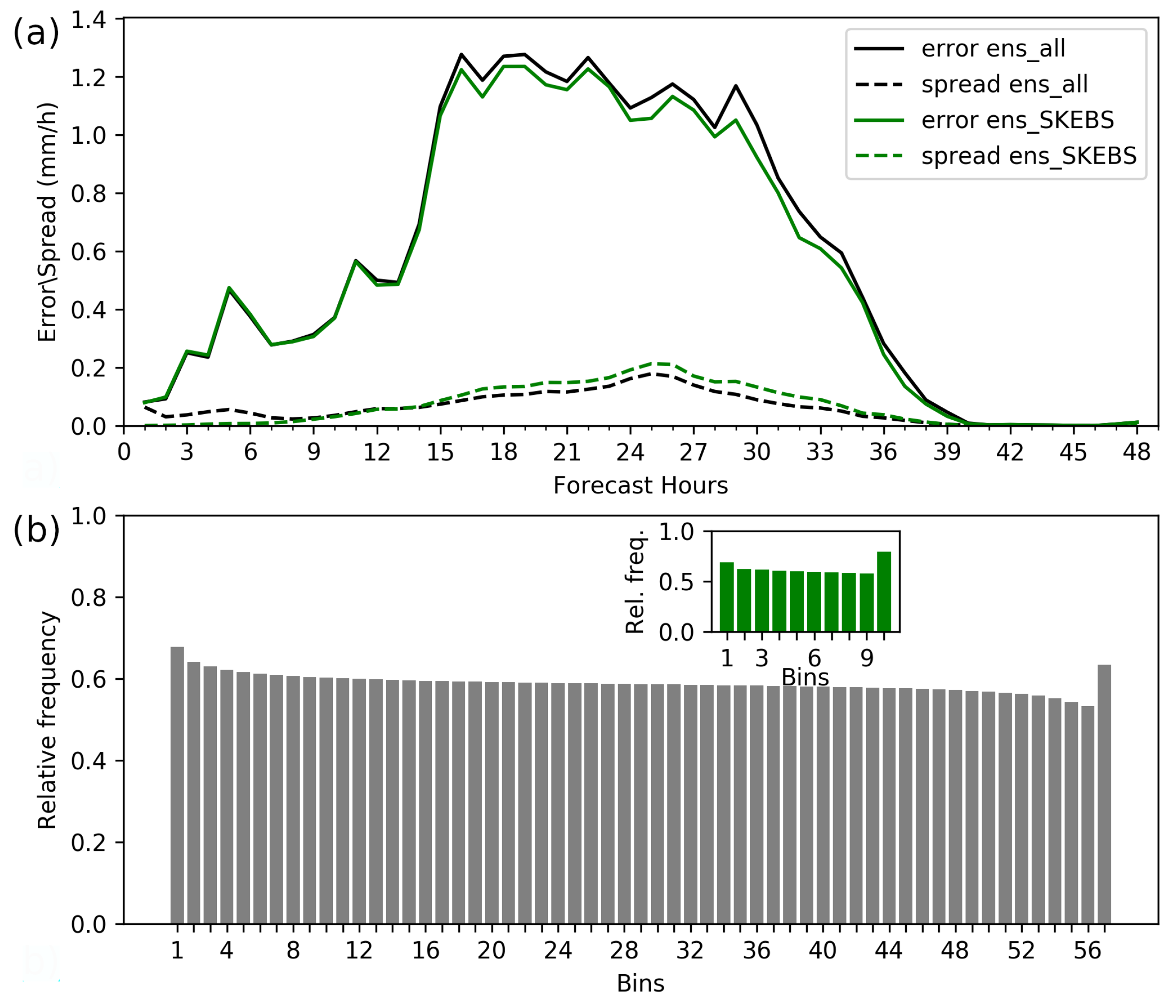
3.2. Verification Analysis

In this Section, we assess each deterministic run’s performance and the ensemble itself as a whole. The verification was performed near the Lopez Zamora Meteorological Station, close to the center of the domain. This point was located in the area where most precipitation occurred. IMERG data were used to extend the precipitation analysis through the entire domain.

The overall behavior of the ensemble members was evaluated by comparing them with each other and analyzing the level of agreement within the simulations. Figure 9 displays the bias computed as the average of the field difference between two members on top, while the bottom map shows the standard deviation of precipitation of all simulations. It can here be observed that all breeding simulations exhibited small differences between them. The same was observed for temperature and pressure (not shown). Despite the localized perturbation growth found in the breeding members coming from SKEBS, these simulations showed the smallest biases. However, there were some differences between the breeding members and the rest of the simulations. SKEBS members showed notable differences between each other. This difference, combined with their positive perturbation growth found earlier, made these members desirable for constructing an EPS. The members with the most substantial overall biases were those associated with random perturbations using CV3. These biases may be related to the amplitude and length scale of the initial perturbations with which these simulations started. This result probably explains why Exp 5 ranked second place in integral IE values. The large biases in these CV3-related members made them outliers that added new, and perhaps unwanted, information. The member Cu09u also showed large biases. Here this member produced less overall precipitation than the other simulations.

Although the advantages of using multiphysics ensembles to increase ensemble spread have been confirmed [26,27], we argue that selecting a suite of physical parameterizations that behave differently enough for the region of interest can be challenging. Instead, using a well-tested, physical parameterization set for one specific region, and applying SKEBS could be sufficient to obtain, at least, a comparative degree of spread amongst these members without the need to consider unrealistic outliers.

The ensemble dispersion can be inferred from the standard deviation (Figure 9b). The areas of higher values coincided with the regions where the WRF model presented more uncertainty due to the thermodynamic instability present in the domain during the study period. Note that in the case of precipitation, the areas with higher dispersion agreed well with those of maximum rainfall shown in Figure 3. For the other variables, this was not the case.

Meanwhile, the biases for water vapor and wind speed were higher and different among all the ensemble members. Figure 10a shows the biases and Figure 10b the standard deviation for the water vapor. Here, the same members found as outliers for precipitation were those with the highest overall bias. The standard deviations of temperature, vapor, pressure, and wind speed exhibited similar patterns. As shown for water vapor, all these variables presented high values eastward of the peninsula’s elevation axis extending toward the northern Gulf of California and south of Arizona. To a lesser extent, such high values were also present along the coasts of California and Baja California. Minimum dispersion occurred windward of the mountain peaks along the peninsula, north of the domain, and over the Pacific Ocean. The water vapor was, spatially, the most uncertain variable in the model. Wind speed (not shown) had less spatial variability but showed the least agreement within the ensemble members regarding its intensity.

Results of the grid point verification at the Lopez Zamora station are presented using Taylor diagrams for precipitation, water vapor mixing ratio, temperature, and pressure, shown in Figure 11a–d, respectively. The radial axis shows the standard deviation (STD), while the azimuth presents Pearson’s correlation coefficient (COR). The red dot represents the observation and reference value. Away from this dot set as the center, gray-dashed circumferences account for the root mean square difference (RMSD).

Precipitation was the variable most sensitive to variations between the ensemble members (see Figure 11). The members showed little dispersion with correlation values around 0.9 and standard deviations slightly above the reference for temperature and pressure. The water vapor mixing ratio exerted a similar behavior, although the STD of all members was slightly below the reference, while COR values fell to 0.8. The overall RMSD values were around unity for these three variables. The latter suggested little value added to the temperature, pressure, and water vapor mixing ratio analysis amongst ensemble members.

The Taylor diagram for precipitation (Figure 11a) showed more dispersion between the members. However, COR values were lower than those for the other variables but are still above 0.6 for most members. Most of the variability was observed along the radial axis and could be represented with the SKEBS members (green marks) alone. Increasing the amount of SKEBS members could contribute to better represent the natural variability of the precipitation in terms of the period analyzed in this case study without the need to use any other perturbation methodology. Duda et al. [20] and Romine et al. [19] also found an increase in the spread produced by SKEBS perturbations in a high-resolution ensemble with seven members over the center of the United States. Moreover, it should be noted that the initial condition perturbation members (yellow, orange, and pink marks) tended to be grouped, showing no dispersion in the Taylor plots. Of those members, the ones using CV3 tended to show outliers indicating the worst deterministic forecasts. However, the overall ensemble mean (brown circle) was strongly determined by this lack of dispersion and the number of breeding members. The STD values were near the reference for the temperature, water vapor, and pressure, but they were almost doubled for precipitation.

In Figure 11a, two additional circular marks appeared. The violet one corresponded to the IMERG precipitation dataset evaluated at a point nearest the station location, and the dark-blue one represented the ERA5-Land dataset [60]. In Figure 11a, both datasets showed similar behavior compared to the precipitation observed in the Lopez Zamora station during the study. The IMERG standard deviation was closer to that of the actual observation (red dot), which was probably related to the coarser, 0.25 degree, resolution of the ERA5 simulations from which this product was derived. Therefore, for this study, we used the IMERG dataset.

IMERG data allowed us to extend the precipitation analysis to about a third of grid points in the domain. However, more importantly, it has been shown that IMERG can be a useful tool for precipitation assessments in areas where in-situ observations are sparse [61,62]. Figure 12a shows the Taylor diagram at a grid point representing the Lopez Zamora station location but using the GPM calibrated precipitation as the reference. Comparing this plot and Figure 11a, it is shown that the statistics of the members in the Taylor plots remained grouped around the ensemble mean (brown circle), with a tendency to stretch along the radial axis. Both the satellite-derived and the actual precipitation gauge measurements presented similar standard deviations below 2 mm/h. However, COR values could be overestimated by 0.1, while the RMSD was underestimated when using IMERG data as a reference. The latter could be related to the smoothing of the precipitation field of IMERG. Figure 12b shows the same statistic information but for the grid point in the analysis domain with maximum average precipitation computed from all ensemble members during the study period. It shows that the higher the ensemble average precipitation, the higher the correlation and errors to IMERG can be. In addition, the dispersion between the statistics of the SKEBS members was maintained, while it was reduced for the breeding members. We mentioned earlier that higher uncertainties were produced in the area where precipitation was more likely to occur. The grid point with maximum average precipitation was expected to be found within this area. Therefore, we deduced that high correlations and errors with respect to IMERG would also be found in regions with high information entropy because it was a measure of uncertainty.

3.3. Verification of the Full Ensemble against the Ensemble of Selected Members

Above, an analysis of individual members was performed. Results showed that the SKEBS members presented positive growth rates and enough information and dispersion to disregard the others. Further analysis used IMERG precipitation data to compare statistics from the overall ensemble (the ensemble accounting for all members: ens_all) and the ensemble made of SKEBS members only (ens_SKEBS).

In this respect, Figure 13 presents the spread-skill diagram in (a), and the rank histogram in (b) [56]. Hourly precipitation data for IMERG were used as a reference against the two-dimensional precipitation fields of the WRF simulations composing the ensembles. These numerical fields were interpolated to match the IMERG resolution in the study domain. Figure 13a provides information on how the ensembles behave by comparing the error (thick) and the spread (dashed) lines. Theoretically, in a perfect ensemble, both lines should be approximately equal. In Figure 13b, the shape of the histogram itself characterized the ensemble spread. A flat histogram would indicate that any member of the ensemble (shown as a bin) was equally likely to produce the observed precipitation. Meanwhile, any tilting would be associated with biases. Bell- and U-shaped histograms are signs of over- and under-spread, respectively.

Figure 13 shows that the ensembles’ precipitation errors are higher than their spreads. In general, the spread increased in line with the error, and the errors did not surpass 1.3 mm/h. It is also shown that the error/spread relation improved for ens_SKEBS during the hours of intense precipitation. The rank histogram shows that both ensembles had a low spread associated with their members not being able to reproduce extreme values. Small tilting towards the left in both ends of these plots was associated with the inherent characteristics of precipitation since it was discrete and contained a mode of no rain. However, if intense precipitation occurred over some discrete points, the model under predicted it. In the same manner, the model tended to produce continuous fields of precipitation, which could overestimate observations of zero rainfall in small amounts. These findings agree with [63], who analyzed the spread-skill relationship for precipitation forecasts and their dependence on the intensity and spatial distribution using a high-resolution ensemble.

A reliability diagram [64] for the overall ensemble (ens_all) is shown in Figure 14a. The thick, black, diagonal line corresponded to a perfect ensemble while the shaded area still indicated reliability. The blue line is computed for the ensemble using a threshold of 0.1 mm to dichotomize precipitation events. Observed frequencies above 20% (dashed line) indicated reliability. The ensemble achieved this, albeit without sharpness (lack of average tilt in the blue curve). This result was expected since low or no precipitation is usually overestimated by most members in areas with a low probability of occurrence or under weak meteorological forcing. On the other hand, when the forcing was strong or in areas where the probability of precipitation is high, most members agreed to produce some precipitation but with no accuracy. For ens_SKEBS (not shown), the same characteristics remained.

The ROC plot [64,65] for the ensembles is shown in Figure 14b. The diagonal black dashed line represented no skill, which accounted for half of the square’s total area defined by the Figure axes. Any other value of the area under the curve (AUC) above 0.5 would indicate that the ensemble skill could be improved, which could be achieved, for example, by parameter tuning, by increasing the number of members, or statistical post-processing. An ensemble with perfect skill would have an AUC of 1.0 squared units indicated by a line going from the origin to the other extreme of the diagonal through the left and top axes. The blue line represented an AUC of 0.75 square units for the whole analysis domain, which confirms that the overall ensemble skill could be improved. However, the curve showed a straight line between the FAR interval (0.15,1.0). This behavior is typical for rare events. Depending on the domain and the temporal-spatial distribution of the precipitation, it may have the characteristics of a rare event. Therefore, the ROC curve was re-computed for a subregion where precipitation was more likely to occur. This subregion was located between 31 and 33 degrees north and from 115 to 118 degrees west. The resulting curve, shown in dashed blue, was more rounded, and the AUC increased to 0.84 square units. This result highlights once again the complexity of the precipitation as a verification variable. At the same time, it shows how unsettled the skill results of an ensemble can be depending on the meteorological forcing linked to a precipitation event. The latter also applies to any deterministic model simulation. For ens_SKEBS, the AUC corresponding to the same subregion was 0.82 square units, which was smaller than that of ens_all by 0.02 square units, mainly due to the difference in the number of members between the two ensembles. The lesser the number of members considered, the rarer the precipitation events could be considered while fixing the area of analysis, as in this case.

These results suggest that the current high-resolution ensemble system’s skill can be improved using only SKEBS members. In addition, increasing the current number of these members could contribute to improving the spread and verification statistics.

4. Summary and Conclusions

To design a convective scale ensemble prediction system in Baja California centered over the Port of Ensenada, 56 different WRF members were analyzed during a high precipitation event. Those members represented initial conditions and model error uncertainties. Within this set, we explored the behavior of random perturbations in the initial conditions derived from two different background error covariance matrices and different wavelengths. Another subset used the stochastic kinetic energy backscatter scheme. Breeding perturbations were included using a 24 h breeding cycle of the day before the simulation start and the member generation methods mentioned above. Lastly, one member was created using physics options different from the rest of the simulations.

The initial condition analysis found that the average spatial growth of the perturbations shows rapid exponential growth of the model errors during the first six hours of the simulation period. Afterwards, the average growth rate remains constant until the end of the simulation. The time and vertical averages of the perturbation growth rates reflect the role of the convective energy and the orographic forcing in the localization of growth patches. The latter is especially true for breeding members coming from SKEBS, and, to a lesser extent, for the SKEBS members because of the continuous injections of energy throughout the simulation period by the parametrization. The rest of the members showed limited growth except for the member with different physics.

Regarding the growth rate analysis, it seems that SKEBS members mimic multiphysics behavior. The results show that the power spectral density profiles of the initial perturbation fields tend to be grouped depending on each member’s origin and the methods used to create the breeding members due to energy conservation. We found an inverse relationship between the overall PSD at the beginning of the simulations and the initial growth rate. This relation is potentially useful for selecting appropriate initial condition perturbations for ensemble generation. However, even the “best” initial condition perturbations are not enough to generate a desirable spread of an ensemble because of the rapid decay of the perturbation growth rates due to the lateral boundary constraints in a limited area model. The dynamical injections of energy, introduced as perturbations to the numerical fields by the SKEBS method, were essential to maintain positive growth rates during the simulation.

The normalized information entropy analysis shows spatially-averaged values under 0.9 for all meteorological variables. For precipitation, a distinct evolution pattern is observed, which is very different from the other variables’ pattern. The precipitation normalized IE maxima are below 0.6 around the 24 h of the simulation period when most precipitation occurred. In addition, time-average IE values show some spatial correlation with the standard deviation. The results found here suggested the need to eliminate redundant information in the ensemble. In this respect, nine experiments were carried out. These experiments led to the conclusion that the normalized IE is maximized using only the members with positive average growth rates during the simulation period. In this experiment, spatially-averaged normalized IE values topped at 0.95 for temperature, water vapor, pressure, and wind speed with similar evolution patterns, while for precipitation, a peak above 0.7 was reached.

Generally, the ensemble presented here is under dispersive, i.e., the ensemble spread does not provide a good estimate of forecast error, with a few outliers such as the members using CV3 random perturbations. These initial perturbations were characterized by large spatial wavelengths, which is probably why they presented the smallest growth rates. The breeding members coming from SKEBS could have some value, particularly in areas of atmospheric instability. Their spread and growth rate could increase after a few breeding cycles, as the literature suggests [12]. However, in this case, it was noted that the domain average growth rate is negative, leading to little dispersion between these members. Moreover, the mean biases between members are small, especially for the breeding members. They are more substantial and more variable among SKEBS simulations, and peak, in absolute terms, for water vapor mixing ratio and wind speed. The average spread of the ensemble is spatially variable with locally higher values, as a response of the atmospheric conditions and characteristics of the simulation domain. For example, the largest dispersion areas of the ensemble precipitation appear in regions with intense rainfall. With water vapor, the spread is larger over the northern Gulf of California. It should be noted, however, that the standard deviation values are rather low. Meanwhile, the other variables show larger spreads leeward of the mountain systems northern of the peninsula and south of California.

For the design of the ensemble proposed for this region, we suggest using only SKEBS members. In addition, increasing the number of these members depending on the computer resources available could benefit the spread of the ensemble and forecast verification statistics. The spread results found in an earlier study for this region [29] should improve following this suggestion. Additionally, evidence was found that post-processing techniques can improve the forecast results of the ensemble. Further investigations will focus on the statistical post-processing in higher resolution ensemble simulations to improve the skill of the quantitative precipitation forecasts.

References

1. Gebhardt, C.; Theis, S.; Krahe, P.; Renner, V. Experimental ensemble forecasts of precipitation based on a convection-resolving model. Atmos. Sci. Lett. 2008, 9, 67–72. [Google Scholar] [CrossRef]
2. Johnson, A.; Wang, X.; Kong, F.; Xue, M. Hierarchical Cluster Analysis of a Convection-Allowing Ensemble during the Hazardous Weather Testbed 2009 Spring Experiment. Part I: Development of the Object-Oriented Cluster Analysis Method for Precipitation Fields. Mon. Weather Rev. 2011, 139, 3673–3693. [Google Scholar] [CrossRef] [Green Version]
3. Duda, J.D.; Wang, X.; Kong, F.; Xue, M. Using Varied Microphysics to Account for Uncertainty in Warm-Season QPF in a Convection-Allowing Ensemble. Mon. Weather Rev. 2014, 142, 2198–2219. [Google Scholar] [CrossRef]
4. Schwartz, C.S.; Romine, G.S.; Smith, K.R.; Weisman, M.L. Characterizing and optimizing precipitation forecasts from a convection-permitting ensemble initialized by a mesoscale ensemble Kalman filter. Weather Forecast. 2014, 29, 1295–1318. [Google Scholar] [CrossRef] [Green Version]
5. Klasa, C.; Arpagaus, M.; Walser, A.; Wernli, H. An evaluation of the convection-permitting ensemble COSMO-E for three contrasting precipitation events in Switzerland. Q. J. R. Meteorol. Soc. 2018, 144, 744–764. [Google Scholar] [CrossRef]
6. Fosser, G.; Kendon, E.; Chan, S.; Lock, A.; Roberts, N.; Bush, M. Optimal configuration and resolution for the first convection-permitting ensemble of climate projections over the United Kingdom. Int. J. Climatol. 2019. [Google Scholar] [CrossRef]
7. Porson, A.N.; Hagelin, S.; Boyd, D.F.A.; Roberts, N.M.; North, R.; Webster, S.; Lo, J.C.F. Extreme rainfall sensitivity in convective-scale ensemble modelling over Singapore. Q. J. R. Meteorol. Soc. 2019, 145, 3004–3022. [Google Scholar] [CrossRef]
8. Clark, A.J.; Kain, J.S.; Stensrud, D.J.; Xue, M.; Kong, F.; Coniglio, M.C.; Thomas, K.W.; Wang, Y.; Brewster, K.; Gao, J.; et al. Probabilistic precipitation forecast skill as a function of ensemble size and spatial scale in a convection-allowing ensemble. Mon. Weather Rev. 2011, 139, 1410–1418. [Google Scholar] [CrossRef] [Green Version]
9. Schellander-Gorgas, T.; Wang, Y.; Meier, F.; Weidle, F.; Wittmann, C.; Kann, A. On the forecast skill of a convection-permitting ensemble. Geosci. Model Dev. 2017, 10, 35–56. [Google Scholar] [CrossRef] [Green Version]
10. Du, J.; Mullen, S.L.; Sanders, F. Short-range ensemble forecasting of quantitative precipitation. Mon. Weather Rev. 1997, 125, 2427–2459. [Google Scholar] [CrossRef]
11. Toth, Z.; Kalnay, E. Ensemble forecasting at NMC: The generation of perturbations. Bull. Am. Meteorol. Soc. 1993, 74, 2317–2330. [Google Scholar] [CrossRef] [Green Version]
12. Toth, Z.; Kalnay, E. Ensemble Forecasting at NCEP and the Breeding Method. Mon. Weather. Rev. 1997, 125, 3297–3319. [Google Scholar] [CrossRef]
13. Leutbecher, M. On ensemble prediction using singular vectors started from forecasts. Mon. Weather Rev. 2005, 133, 3038–3046. [Google Scholar] [CrossRef]
14. Krishnamurti, T.N.; Kishtawal, C.M.; Zhang, Z.; LaRow, T.; Bachiochi, D.; Williford, E.; Gadgil, S.; Surendran, S. Multimodel ensemble forecasts for weather and seasonal climate. J. Clim. 2000, 13, 4196–4216. [Google Scholar] [CrossRef]
15. Evans, R.E.; Harrison, M.S.J.; Graham, R.J.; Mylne, K.R. Joint medium-range ensembles from the Met. Office and ECMWF systems. Mon. Weather Rev. 2000, 128, 3104–3127. [Google Scholar] [CrossRef]
16. Buizza, R.; Milleer, M.; Palmer, T.N. Stochastic representation of model uncertainties in the ECMWF ensemble prediction system. Q. J. R. Meteorol. Soc. 1999, 125, 2887–2908. [Google Scholar] [CrossRef]
17. Shutts, G.J. A kinetic energy backscatter algorithm for use in ensemble prediction systems. Q. J. R. Meteorol. Soc. 2005, 612, 3079–3102. [Google Scholar] [CrossRef] [Green Version]
18. Bouttier, F.; Vié, B.; Nuissier, O.; Raynaud, L. Impact of stochastic physics in a convection-permitting ensemble. Mon. Weather Rev. 2012, 140, 3706–3721. [Google Scholar] [CrossRef]
19. Romine, G.S.; Schwartz, C.S.; Berner, J.; Fossell, K.R.; Snyder, C.; Anderson, J.L.; Weisman, M.L. Representing Forecast Error in a Convection-Permitting Ensemble System. Mon. Weather Rev. 2014, 142, 4519–4541. [Google Scholar] [CrossRef] [Green Version]
20. Duda, J.F.; Wang, X.; Kong, F.; Xue, M.; Berner, J. Impact of a Stochastic Kinetic Energy Backscatter Scheme on Warm Season Convection-Allowing Ensemble Forecasts. Mon. Weather Rev. 2016, 144, 1887–1908. [Google Scholar] [CrossRef]
21. Berner, J.; Achatz, U.; Batte, L.; Bengtsson, L.; de la Cámara, A.; Christensen, H.M.; Colangeli, M.; Coleman, D.R.B.; Crommelin, D.; Dolaptchiev, S.I.; et al. Stochastic parameterization: Toward a new view of weather and climate models. Bull. Am. Meteorol. Soc. 2017, 98, 565–588. [Google Scholar] [CrossRef] [Green Version]
22. Du, J.; Berner, J.; Buizza, R.; Charron, M.; Houtekamer, P.; Hou, D.; Isidora, J.; Mu, M.; Wang, X.; Wei, M.; et al. Ensemble methods for meteorological predictions. NCEP Office Notes 2018, 493. [Google Scholar] [CrossRef]
23. Bowler, N.E. Comparison of error breeding, singular vectors, random perturbations and ensemble Kalman filter perturbation strategies on a simple model. Tellus 2006, 58A, 538–548. [Google Scholar] [CrossRef] [Green Version]
24. Magnusson, L.; Källén, E.; Nycander, J. Initial state perturbations in ensemble forecasting. Nonlin. Processes Geophys. 2008, 15, 751–759. [Google Scholar] [CrossRef]
25. Greybush, S.J.; Saslo, S.; Grumm, R. Assessing the ensemble predictability of precipitation forecasts for the January 2015 and 2016 East Coast winter storms. Weather Forecast. 2017, 32, 1057–1078. [Google Scholar] [CrossRef]
26. Li, C.H.; Berner, J.; Hong, J.S.; Fong, C.T.; Kuo, Y.H. The Taiwan WRF Ensemble Prediction System: Scientific Description, Model-Error Representation and Performance Results. Asia-Pac. J. Atmos. Sci. 2019. [Google Scholar] [CrossRef] [Green Version]
27. Berner, J.; Fossel, K.R.; Ha, S.Y.; Hacker, J.P.; Snyder, C. Increasing the skill of probabilistic forecasts: understanding performance improvements from model-error representations. Mon. Weather Rev. 2015, 143, 1295–1320. [Google Scholar] [CrossRef]
28. Jankov, I.; Berner, J.; Beck, J.; Jiang, H.; Olson, J.B.; Grell, G.; Smirnova, T.G.; Benjamin, S.G.; Brown, J.M. A performance comparison between multiphysics and stochastic approaches within a North American RAP ensemble. Mon. Weather Rev. 2017, 145, 1161–1179. [Google Scholar] [CrossRef]
29. Méndez-Turrubiates, R.F.; Gross, M.; Magar, V. Local Quantitative Precipitation Forecasts with Minimal Data Requirement – An Ensemble Approach. Weather Forecast. 2020, 35, 821–839. [Google Scholar] [CrossRef]
30. Guo, Y.R.; Lin, H.C.; Ma, X.X.; Huang, X.Y.; Terng, C.T.; Kuo, Y.H. Impact of WRF-Var (3DVar) background error statistics on typhoon analysis and forecast. In Seventh WRF Users’ Workshop; NCAR: Boulder, CO, USA, 2006. [Google Scholar]
31. Pannekoucke, O.; Berre, L.; Desroziers, G. Background-error correlation length-scale estimates and their sampling statistics. Q. J. R. Meteorol. Soc. A J. Atmos. Sci. Appl. Meteorol. Phys. Oceanogr. 2008, 134, 497–508. [Google Scholar] [CrossRef] [Green Version]
32. National Centers for Environmental Prediction National Weather Service, NOAA, U.S. Department of Commerce (NCEP). NCEP North American Mesoscale (NAM) 12 km Analysis; Research Data Archive at the National Center for Atmospheric Research, Computational and Information Systems Labortory: Boulder, CO, USA, 2014. [CrossRef]
33. Huffman, G.J.; Bolvin, D.T.; Braithwaite, D. Integrated Multi-SatellitE Retrievals for GPM (IMERG). NASA’s Precipitation Processing Center. 2014. Available online: https://storm.pps.eosdis.nasa.gov/storm/ (accessed on 8 September 2020).
34. Skamarock, W.C.; Klemp, J.B.; Dudhia, J.; Gill, D.O.; Barker, D.M.; Wang, W.; Power, J.G. A description of the Advanced Research WRF version 3. NCAR Technical Note 2008. [Google Scholar] [CrossRef]
35. Stensrud, D.J. Parameterization Schemes: Keys to Understanding Numerical Weather Prediction Models; Cambridge University Press: Cambridge, UK, 2009. [Google Scholar]
36. Hsiao, L.F.; Yang, M.J.; Lee, C.S.; Kuo, H.C.; Shih, D.S.; Tsai, C.C.; Wang, C.J.; Chang, L.Y.; Chen, D.Y.C.; Feng, L.; et al. Ensemble forecasting of typhoon rainfall and floods over a mountainous watershed in Taiwan. J. Hydrol. 2013, 506, 55–68. [Google Scholar] [CrossRef] [Green Version]
37. Thompson, G.; Field, P.R.; Rasmussen, R.M.; Hall, W.D. Explicit Forecasts of Winter Precipitation Using an Improved Bulk Microphysics Scheme. Part II: Implementation of a New Snow Parameterization. Mon. Weather Rev. 2008, 136, 5095–5115. [Google Scholar] [CrossRef]
38. Tan, E. Microphysics parameterization sensitivity of the WRF Model version 3.1.7 to extreme precipitation: evaluation of the 1997 New Year’s flood of California. Geosci. Model Dev. Discuss. 2016, 1–29. [Google Scholar] [CrossRef] [Green Version]
39. Hong, S.Y.; Noh, Y.; Dudhia, J. A new vertical diffusion package with an explicit treatment of entrainment processes. Mon. Weather Rev. 2006, 134, 2318–2341. [Google Scholar] [CrossRef] [Green Version]
40. Hu, X.M.; Nielsen-Gammon, J.W.; Zhang, F. Evaluation of three planetary boundary layer schemes in the WRF model. J. Appl. Meteor. Climatol. 2010, 49, 1831–1844. [Google Scholar] [CrossRef] [Green Version]
41. Iacono, M.J.; Delamere, J.S.; Mlawer, E.J.; Shephard, M.W.; Clough, S.A.; Collins, W.D. Radiative forcing by long-lived greenhouse gases: Calculations with the AER radiative transfer models. J. Geophys. Res. Atmos. 2008, 113. [Google Scholar] [CrossRef]
42. Jiménez, P.A.; Dudhia, J.; González-Rouco, J.F.; Navarro, J.; Montávez, J.P.; García-Bustamante, E. A revised scheme for the WRF surface layer formulation. Mon. Weather Rev. 2012, 140, 898–918. [Google Scholar] [CrossRef] [Green Version]
43. Fairall, C.W.; Bradley, E.F.; Hare, J.E.; Grachev, A.A.; Edson, J.B. Bulk parameterization of air–sea fluxes: Updates and verification for the COARE algorithm. J. Clim. 2003, 16, 571–591. [Google Scholar] [CrossRef]
44. Lynch, P. The Dolph–Chebyshev window: A simple optimal filter. Mon. Weather Rev. 1997, 125, 655–660. [Google Scholar] [CrossRef] [Green Version]
45. Kain, J.S. The Kain–Fritsch convective parameterization: An update. J. Appl. Meteorol. 2004, 43, 170–181. [Google Scholar] [CrossRef] [Green Version]
46. Hong, S.Y.; Dudhia, J.; Chen, S.H. A revised approach to ice microphysical processes for the bulk parameterization of clouds and precipitation. Mon. Weather Rev. 2004, 132, 103–120. [Google Scholar] [CrossRef]
47. Descombes, G.; Auligné, T.; Vandenberghe, F.; Barker, D.M.; Barre, J. Generalized background error covariance matrix model (GEN_BE v2. 0). Geosci. Model Dev. 2015, 8, 669–696. [Google Scholar] [CrossRef] [Green Version]
48. Parrish, D.F.; Derber, J.C. The National Meteorological Center’s spectral statistical interpolation analysis system. Mon. Weather Rev. 1992, 120, 1747–1763. [Google Scholar] [CrossRef]
49. Berner, J.; Shutts, G.J.; Leutbecher, M.; Palmer, T.N. A spectral stochastic kinetic energy backscatter scheme and its impact on flow-dependent predictability in the ECMWF ensemble prediction system. J. Atmos. Sci. 2009, 66, 603–626. [Google Scholar] [CrossRef]
50. Lorenz, E.N. Deterministic Nonperiodic Flow. J. Atmos. Sci. 1963, 20, 130–141. [Google Scholar] [CrossRef] [Green Version]
51. Blázquez, J.; Pessacg, N.L.; Gonzalez, P.L.M. Simulation of a baroclinic wave with the WRF regional model: Sensitivity to the initial conditions in an ideal and a real experiment. Meteorol. Appl. 2013, 20, 447–456. [Google Scholar] [CrossRef]
52. DelSole, T. Predictability and information theory. Part II: Imperfect forecasts. J. Atmos. Sci. 2005, 62, 3368–3381. [Google Scholar] [CrossRef]
53. MacKay, D.J.C. Information Theory, Inference and Learning Algorithms; Cambridge University Press: Cambridge, UK, 2003. [Google Scholar]
54. Ma, S.; Chen, C.; He, H.; Xiang, J.; Chen, S.; Li, Y.; Jiang, Y.; Wu, D.; Luo, H. An Analysis on Perturbation Features of Convection-Allowing Ensemble Prediction Based on the Local Breeding Growth Mode. Weather Forecast. 2019, 34, 289–304. [Google Scholar] [CrossRef]
55. Silverman, B.W. Density Estimation for Statistics and Data Analysis; Chapman & Hall/CRC: Boca Raton, FL, USA, 1998. [Google Scholar]
56. Wilks, D.S. Statistical Methods in the Atmospheric Sciences, 3rd ed.; Elsevier: Amsterdam, The Netherlands, 2011; p. 676. [Google Scholar]
57. Hohenegger, C.; Schär, C. Predictability and Error Growth Dynamics in Cloud-Resolving Models. J. Atmos. Sci. 2007, 64, 4467–4478. [Google Scholar] [CrossRef]
58. Kühnlein, C.; Keil, C.; Craig, G.C.; Gebhardt, C. The impact of downscaled initial condition perturbations on convective-scale ensemble forecasts of precipitation. Q. J. R. Meteorol. Soc. 2014, 140, 1552–1562. [Google Scholar] [CrossRef]
59. Trevisan, A. Impact of Transient Error Growth on Global Average Predictability Measures. J. Atmos. Sci. 1993, 50, 1016–1028. [Google Scholar] [CrossRef]
60. Copernicus Climate Change Service (C3S). ERA5-Land Reanalysis. Available online: http://doi.org/10.24381/cds.e2161bac (accessed on 8 September 2020).
61. Mayor, Y.G.; Tereshchenko, I.; Fonseca-Hernández, M.; Pantoja, D.; Montes, J. Evaluation of error in IMERG precipitation estimates under different topographic conditions and temporal scales over Mexico. Remote Sens. 2017, 9, 503. [Google Scholar] [CrossRef] [Green Version]
62. Asong, Z.; Razavi, S.; Wheater, H.S.; Wong, J.S. Evaluation of integrated multisatellite retrievals for GPM (IMERG) over southern Canada against ground precipitation observations: A preliminary assessment. J. Hydrometeorol. 2017, 18, 1033–1050. [Google Scholar] [CrossRef]
63. Chen, X.; Yuan, H.; Xue, M. Spatial spread-skill relationship in terms of agreement scales for precipitation forecasts in a convection-allowing ensemble. Q. J. R. Meteorol. Soc. 2017, 144. [Google Scholar] [CrossRef]
64. Jolliffe, I.T.; Stephenson, D. Forecast Verification. A Practitioner’s Guide in Atmospheric Science, 2nd ed.; Wiley and Sons Ltd.: Hoboken, NJ, USA, 2012. [Google Scholar]
65. Abhilash, S.; Sahai, A.K.; Borah, N.; Joseph, S.; Chattopadhyay, R.; Rajeevan, M.; Mapes, B.E.; Kumar, A. Improved Spread–Error Relationship and Probabilistic Prediction from the CFS-Based Grand Ensemble Prediction System. J. Appl. Meteorol. Climatol. 2015, 54, 1569–1578. [Google Scholar] [CrossRef]
Figure 1. Case Study area. The star with the ZMS label near the center of the domain shows the approximate location of the Lopez Zamora Meteorological Station.
Atmosphere 11 00973 g001
Figure 2. Observation data from the Lopez Zamora Station: (a) precipitation in mm/h, (b) water vapor mixing ratio in g/kg, (c) temperature in degree celsius, and (d) pressure in hPa. The horizontal axis represents the hours after 27 February 2017 at 00 UTC.
Atmosphere 11 00973 g002
Figure 3. Hourly precipitation estimates (in mm/h) from IMERG. Valid for 27 February 2017 at 19 UTC.
Atmosphere 11 00973 g003
Figure 4. The growth rate of the perturbations for each ensemble member during the simulation period starting at 00Z on 27 February 2017. Light shadings represent the vertical standard deviations.
Atmosphere 11 00973 g004
Figure 5. 1-D power spectral density in dB of the water vapor (a), temperature (b), pressure (c), and wind speed (d) perturbation fields in the sigma level closest to the surface at 00Z on 27 February 2017 for each member of the ensemble system. The frequency domain (horizontal axis) is expressed in terms of distance in km.
Atmosphere 11 00973 g005
Figure 6. Time and vertically-averaged growth rate of the perturbations during the simulation period starting at 00Z on 27 February 2017. The members presented are Cu09ur (a), Op31ur (b), Op71ur (c), Su01ur (d), Su05ur (e), Bp31po (f), Bp71po (g), Bp01us (h), Bp05us (i).
Atmosphere 11 00973 g006
Figure 7. Temporal evolution (a) and spatial distribution (bf) of information entropy computed for rain, temperature, water vapor, pressure, and wind speed from (bf), respectively. Valid for the simulation period starting at 00Z on 27 February 2017.
Atmosphere 11 00973 g007
Figure 8. Temporal evolution of the information entropy computed for rain, temperature, water vapor, pressure, and wind speed for the nine experiments set in Table 4. The experiments appear ordered from (ai), respectively. Valid for the simulation period starting at 00Z on 27 February 2017.
Atmosphere 11 00973 g008
Figure 9. Overall bias (a) and standard deviation (b) of all members for precipitation in mm/h. Valid for the simulation period starting at 00Z on 27 February 2017.
Atmosphere 11 00973 g009
Figure 10. Overall bias (a) and standard deviation (b) of all members for water vapor mixing ratio in g/kg. Valid for the simulation period starting at 00Z on 27 February 2017.
Atmosphere 11 00973 g010
Figure 11. Taylor diagrams for (a) precipitation, (b) water vapor mixing ratio, (c) temperature and (d) pressure computed from hourly data from the Lopez Zamora Meteorological Station used as a reference. WRF data is taken from the domain point closest to the station location. Valid for the simulation period starting at 00Z on 27 February 2017. Dark blue and violet circles in (a) correspond to ERA5-Land, and IMERG datasets evaluated at the point closest to the station location, respectively.
Atmosphere 11 00973 g011
Figure 12. Taylor diagrams for precipitation computed from IMERG hourly data used as a reference. WRF data is taken from (a) the domain point closest to the Lopez Zamora station location, and (b) the point of maximum average precipitation from all members. Valid for the simulation period starting at 00Z on 27 February 2017.
Atmosphere 11 00973 g012
Figure 13. (a) the spread-skill diagram and (b) the rank histogram plot for precipitation using hourly IMERG data as observations for the WRF domain. Black lines and bars correspond to the overall ensemble, while the green ones are for the ensemble considering Stochastic Kinetic Energy Backscatter parameterization (SKEBS) members only. Valid for the simulation period starting at 00Z on 27 February 2017.
Atmosphere 11 00973 g013
Figure 14. (a) the reliability diagram and (b) the ROC plot for precipitation using hourly IMERG data as observations for the WRF domain. Blue lines correspond to the overall ensemble, while the green one are for the ensemble considering SKEBS members only. Valid for the simulation period starting at 00Z on 27 February 2017.
Atmosphere 11 00973 g014