1. Introduction
The impact of odour emission sources on sensitive receptors is a hotly debated topic in recent years. For wastewater treatment plants (WWTPs), because of their proximity to sensitive elements and their location in urban and territorial contexts, an olfactory impact evaluation strategy is required, to limit harassments on the surrounding area and to ensure the correct process management. Odour impact assessment presents multiple aspects of complexity. The scientific community agrees in recommending an integrated multi-tool assessment strategy, which supports both qualitative and quantitative analyses, atmospheric dispersion modelling, odour measurement in ambient air, population monitoring as well as the mitigation and control actions of olfactory harassment [
1,
2]. Odour impact assessment is carried out through the following phases: sampling, characterization, odour emission rate (OER) calculation, atmospheric dispersion modelling and impact evaluation [
3].
Recently, a significant contribution to the knowledge of odour sampling methods and tools was brought by research, deepening all odour impact assessment stages and the representativeness requirements that the results must have. Odour sampling and characterization are two critical evaluation phases of the assessment. Their accuracy and representativeness, especially related to measuring instruments and type of analysis, strongly influence the subsequent implementation phases of the assessment [
4]. Sensorial analyses are necessary for odour dispersion modelling. The European technique is dynamic olfactometry (DO), regulated by the EN13725: 2004 standard. In this method, the dilution degree necessary to reach the olfactory panel threshold is assessed. Even though the topic of uncertainty relevant to olfactometry is still debated among the scientific community, some studies are proving that the uncertainty of dynamic olfactometry can be estimated between one fourth and fourfold of an actual measurement value [
5,
6].
The odour emission rate calculation is mainly linked to the emission conditions within the sampling devices. Area sources are commonly sampled with hood methods. Hoods can be static or dynamic, for active and passive source sampling, respectively. The most common dynamic hoods are wind tunnels (WTs) and flow chambers (FCs).
In the atmospheric dispersion modelling phase, the results depend on the model choice and settings, but also on the quality of the input data. The type of model choice is a crucial aspect. This is linked to the features of the simulation domain and the scope of the analysis [
7]. To properly evaluate these aspects, it is necessary to conduct a careful study domain analysis, related to the area orography and meteorology, but also emission sources and potentially sensitive receptors. The quality of the incoming meteorological data is also a fundamental factor. The scientific community does not agree on the simulation interval choice: some international jurisdictions prescribe a seasonal or multi-year evaluation duration, believing that it best represents the variability of the emissive and meteorological sources’ conditions [
8].
Finally, the interpretation of the results is based on standardized assumptions on impact evaluation. The time series of odour concentration provided by dispersion models must be evaluated by odour impact criteria (OIC). The OIC are defined by an odour concentration threshold (C
T), the exceedance probability of this threshold (p
T) and the averaging time used to predict the concentrations (A
T) [
9]. If the OIC are specified for an averaging time shorter than 1 h, the peak-to-mean factor (P/M) is commonly applied. The P/M factor allows taking into account the fluctuations of the odour concentrations, which are linked to the atmospheric turbulence and the olfactory sensitivity of the human nose. Applying a P/M factor is simple, but it has a high degree of approximation compared to reality. In many countries, regulations adopt a constant factor. However, concentration fluctuations depend on multiple factors, such as the emissions variability, the source type, the atmospheric stability class and the receptor-source distance.
The results of the application of OIC with odour dispersion modelling are usually reported through the calculation of separation distances. The separation distance is intended to encompass the area within which odour annoyance can be expected, relying on a certain level of protection [
10]. The definition of separation distances can be regarded as a practical approach for decision-making on odour pollution because it easily communicates for all stakeholders the area within which odour annoyance can be expected [
11].
Previous studies showed that different national and local administrations adopted a wide variety of different parameter combinations [
12]. In general, the preferred combinations are either low odour concentration thresholds/high exceedance probabilities or vice versa [
13]. Nevertheless, the theme complexity led to different approaches and instruments, resulting in a lack of homogeneity between regulations [
12]. Besides, the assessment procedures are often incomplete or lack precise information, generating variability in the results. This variability represents the object of the present study.
The objective of this research work was to evaluate the influence of the uncertainties related to some individual stages of odour impact assessment in the application of the current regulatory criteria. The study focused on two main aspects of the assessment. The first was the meteorology data used in dispersion modelling. The second was the open field correction method for wind velocity used in the calculation of OERs. A WWTP located in Northern Italy, whose odour emissions sources were measured in previous campaigns conducted in 2019, was considered as a case study. The evaluation procedure was established by following the guidelines of the Northern Italian regions, which are based on olfactometry analysis according to the European EN13725 standard [
14]. Odour dispersion modelling was carried out using the CALPUFF software.
This study was structured by developing a reference impact assessment and simulation according to the Lombardy Region guidelines [
15], and subsequently running alternative simulations with a modified meteorology and odour emission rate (OER) characterization. This paper is structured as follows: the methodology and a description of the reference and alternative simulations are reported in
Section 2; the results are reported in
Section 3; results are discussed in
Section 4; and, finally, some conclusive remarks are reported in
Section 5.
2. Methodology
In the present study, the odour impact assessment was based on the maximum impact standard, on which the regulations of many states (including Italy) rely on. In this approach, concentrations deriving from the dispersion modelling analysis are evaluated by applying the following odour impact criteria (OIC) [
12]: odour concentration threshold, percentile compliance level, and averaging time for calculating the concentrations.
The study was structured as follows. Firstly, a reference simulation was conducted following Lombardy Region guidelines. Alternative simulations were then made, considering the same modelling domain and emission sources, and alternative simulations aimed at evaluating the impacts on the separation distances of the two factors. The first factor is the meteorology data used in dispersion modelling. Simulations were carried out for two different years (2018 and 2019) to visualize the influence of meteorology on the obtained results. The second factor that was considered is the open field correction method for wind velocity used in the calculation of OERs. To this end, simulations were repeated using three correction methods. The description of the reference and alternative simulations is reported in
Table 1. The description of the studied WWTP and the adopted methodology are reported in the following sub-sections.
2.1. Study Site and Odour Sampling
The WWTP is located in Northern Italy. The site morphology is mainly sub-flat, with a slight slope in the south-east direction towards the river near the plant border. In the eastern part of the domain there are some reliefs. The plant is surrounded by two towns, located NW and SE, respectively. The closest residential area is located 1 km to the plant boundary in the direction NW. The WWTP consists of a line for wastewater treatment and one line for sludge treatment. The wastewater line is made up of the following processes: grid screens, grit and grease removal, primary sedimentation, anoxic and aeration basins, secondary sedimentation and final filtration (
Figure 1). The wastewater treatment process generates an amount of primary and secondary sludge with an average TS content of 1%, which is sent to the sludge treatment units. The sludge treatment line consists of the following units: pre-thickening, mesophilic anaerobic digestion, post-thickening and final dewatering.
A weather monitoring station was installed onsite. The station is composed of the following components:
an ultra-sonic biaxial anemometer, installed at a height of 10 m above ground;
a global class 2 radiometer;
a temperature sensor PT100 1/3 DIN, with a non-vented anti-radiation shield;
a hygrometer with a non-vented anti-radiation shield;
a tilt-out tray pluviometer;
a barometer;
a Campbell CR800 data logging system.
The data logging system provides average values of the weather variables over 10-min intervals.
2.2. Odour Measurements
Odour sampling was carried out at the plant in January 2019. This work used the olfactometry analysis results to calculate the emission rates, as required by EN13725: 2004 standard [
14]. Air samples from passive area sources (referred to as P2, P3, P5 and P6 in
Figure 1) were collected employing a wind tunnel (WT) and following the standard procedure. The WT sampling flow was 2.5 m
3 h
−1, corresponding to an average velocity of 0.035 m s
−1. In addition to the area sources, two volumetric sources were monitored (referred to as P1 and P4 in
Figure 1). The first was the plant inlet, a closed channel where the incoming wastewater is conveyed to the preliminary treatments. Some openings are present on this channel that are potential odour sources. The second was in correspondence of the sludge dehydration section, a closed building in which all the air collected in the sludge treatment line is treated with a wet scrubber. Sampling was done by placing small tubes that correspond to the building openings, and collecting the air in Nalophan bags with the use of a pump. Single samples and a replicate were collected from each source. Odour concentrations were determined in an ODOURNET TO8 olfactometer according to standard EN 13725: 2004.
2.3. OER Calculation
In the reference simulation of the present study, the OER was calculated following the indications provided by the Italian regional technical guidelines. The OER inside the WT (
OERWT, OU s
−1) was calculated from the specific odour emission rate (SOER), as follows (Equations (1) and (2)):
where
SOER is the specific odour emission rate (OU m
−2 s
−1),
Qeffl is the effluent volumetric flow rate leaving the hood (m
3 s
−1),
Abase is the instrument base area (m
2) and
Aemiss is the emission source area (m
2). The values of the parameters of the WT are reported in
Table 2. Values of the
OERWT for each of the area sources are reported in
Table 3.
To calculate the hourly values of the OER,
OERWT was corrected to account for open field conditions [
16]. The main uncertainty of this phase is linked to the significance of the relationship that allows obtaining the emissive flow in the open field starting from that recorded within the dynamic hoods [
17]. In the Italian regulations, a correlation dependent on the relationship between the actual wind speed at the dynamic hood height (
v1) and that of the air flowed inside (
v0) is proposed according to Equation (3):
The dependence on the square root is a simplification since it relates to the laminar flow condition on a flat surface. Some authors [
18] proposed a modification to the equation to improve how the dependence between the emission speed and the wind speed in turbulent conditions is expressed (Equation (4)):
In addition to changing the proportionality factor, the correlation contained a corrected value of the wind speed inside the hood (v0*), taking into account the geometric characteristics of the device.
The OER estimation is closely related to the wind speed profile adopted to obtain
v1 at the flow hood height. In this study, three different wind profile models were evaluated: the power law, the logarithmic law (log law) and the Deaves–Harris correlation (D–H law). The power law does not require the knowledge of complex meteorological data, but the stability class and the prevalent type of land-use class of the surface must be known, expressed through the
α parameter [
19] (Equation (5)):
where
v1 is the wind speed at the flow hood height (m s
−1),
v2 is the wind speed at the meteorological station height (m s
−1),
h1 is the flow hood height (1 m),
h2 is the meteorological station height (10 m) and
α is Hellman’s parameter (-). Values of
α proposed by Hanna et al. [
20] for rural areas were considered. These values, which depend on the atmospheric stability class, are reported in
Table 4. The power law is typically valid in the 30–300 m range, but not for the upper and lower limits of the PBL. Although it is the most used, it does not provide a detailed estimate of the speed at low heights (1–10 m).
The logarithmic law (Equation (6)) was observed to be more suitable for the velocity profile evaluation close to the ground level since it accounts for friction velocity
u* and surface roughness
z0. Furthermore, unlike the power law, it does not constitute an empirical expression as it is derived from similarity theory, according to
where
u* is the friction velocity (m s
−1),
Kv is Von Kármán’s constant (0.41),
z0 is the surface roughness length (0.625 m),
Lm is the Monin–Obukhov length (m) and
ψ is a stability factor, related to the atmospheric stability class (-). The values of the parameters in Equation (6) were extracted by the output of the CALMET simulation. The CALMET model follows the approach introduced by Holtslag and van Ulden [
21], where the calculation of
u*,
Lm and
ψ are differentiated depending on stable and unstable atmospheric conditions. More details can be found in the CALMET user’s manual [
22].
The D–H correlation, also known as the logarithmic with parabolic defect model equation, is defined as reported in Equation (7):
where
H is the equilibrium boundary layer height, equal to
(m);
fc is the Coriolis’ parameter, equal to 2Ωsin(
φ) (s
−1); Ω is the Earth rotation rate, equal to 7.2921∙10
−5 (rad s
−1); and
φ is the latitude (rad). The D–H law is an extension of the previously analysed laws since it includes both scale parameters
u* and
z0 (inherited from the logarithmic profile) and the PBL height parameter. For these reasons [
19], the D–H law can accurately describe the entire PBL and also represent its upper and lower boundary conditions. However, the applicability of this correlation has still to be studied. Cook [
19] pointed out that, in the wind speeds design range, the correspondence between the D–H and power law models is to be considered excellent.
For the volumetric sources, since it was not possible to measure the airflow rate from the building openings, the OER was calculated starting with the hourly air exchange rate (Equation (8)). According to the information provided by the plant operator, an exchange rate equal to 10 h
−1 was assumed.
where
Cod is the odour concentration (OU m
−3), AER is the air exchange rate (h
−1) and
V is the source volume (m
3).
2.4. Odour Impact Assessment
In Italy, as well as other countries worldwide, compliance assessment takes the form of modelling. By analysing the impact maps and the extension of overcoming isopleths, the assessment must understand the measures to be taken to avoid that smell significantly impacts on the receptors.
In this study, the dispersion modelling phase was carried out using CALPUFF [
23]. CALPUFF contains algorithms for modelling the following aspects: puff splitting and merging, building, stack-tip downwash effects, dry and wet deposition, wind shear, chemical transformations, partial penetration into the inversion layers and interaction with complex areas. A detailed plume rise schematization and different puff sampling ways are provided; they can adapt to wind conditions and the presence of buildings.
Technical guidelines require simulations of at least one-year duration and recommend a domain geometry choice that allows to include all potential receptors. Simulations were conducted on a square domain of 16.2 km × 16.2 km, with 10 vertical layers and a 200 m grid step. Surface meteorological data were collected by the weather monitoring station installed onsite. Wind calm conditions were not excluded for the dispersion calculation. Upper air data were collected from radiosounding measurements located at the Milano Linate Airport. Weather observations were first processed with the CALMET model. The area is characterized by mainly agricultural land use. Depletion processes (dry and wet deposition, chemical transformations) were not set up since their effect on atmospheric removal may be considered negligible at this scale of analysis [
24]. The same regulatory indications suggest this choice for olfactory impact studies.
Concerning the OIC, the levels of protection are respected through three different approaches: adjust the odour concentration threshold (C
T), adjust the exceedance probability of this threshold (p
T) and introduce correction factors related to the hedonic tone of the emissions [
11,
25]. In some countries, C
T is assumed as a constant value, whereas p
T is varied depending on location and emission offensiveness. Other countries adopted a constant p
T and modify the C
T for adjusting the criteria to the required level of protection. Previous studies analysing the international regulatory framework indicated three general different groups: a high C
T combined with a low p
T (e.g., C
T = 10 OU m
−3; p
T = 1%); a low C
T combined with a high p
T (e.g., C
T = 1 OU m
−3; p
T = 10%); and a low C
T combined with a low p
T (e.g., C
T = 1 OU m
−3; p
T = 1%).
In the Northern Italian regions, the maximum impact standard is based on the frequency with which a given C
T is exceeded. Three odour impact criteria must be reported in the concentration maps [
15]: 1 OU m
−3, 3 OU m
−3 and 5 OU m
−3. It is defined that 50% of the population perceives the odour at 1 OU m
−3; 85% of the population perceives the odour at 3 OU m
−3; and 90–95% of the population perceives the odour at 5 OU m
−3. These values were derived from the study of Nicell [
26]. Analogously to many other member states of the European Union, the Italian guidelines set the 98th percentile (p
T = 2%) for odour modelling [
12]. The work of Sommer-Quabach et al. [
13] showed that for low exceedance probabilities, such as p
T ≤ 2%, the separation distance has the potential to be driven by a few distinct, uncommon meteorological conditions. To convert from hourly concentrations to short-term odour peaks, a P/M factor of 2.3 was applied. An element of uncertainty [
12] of the Italian standards is the fact that the exceeding criteria do not provide any indication of the average time to which the peak concentrations is referred. Previous works [
27] demonstrated that the P/M factor depends on several parameters, like the stability of the atmosphere, intermittency, travel time or distance from the source. Countries like Australia [
28] or Austria [
29] introduced variable P/M values. Variable P/M were also implemented in the Austrian Odour Dispersion Model (AODM), the regulatory Austrian Gaussian model and in the German Lagrangian model LASAT [
10].
3. Results
As reported in
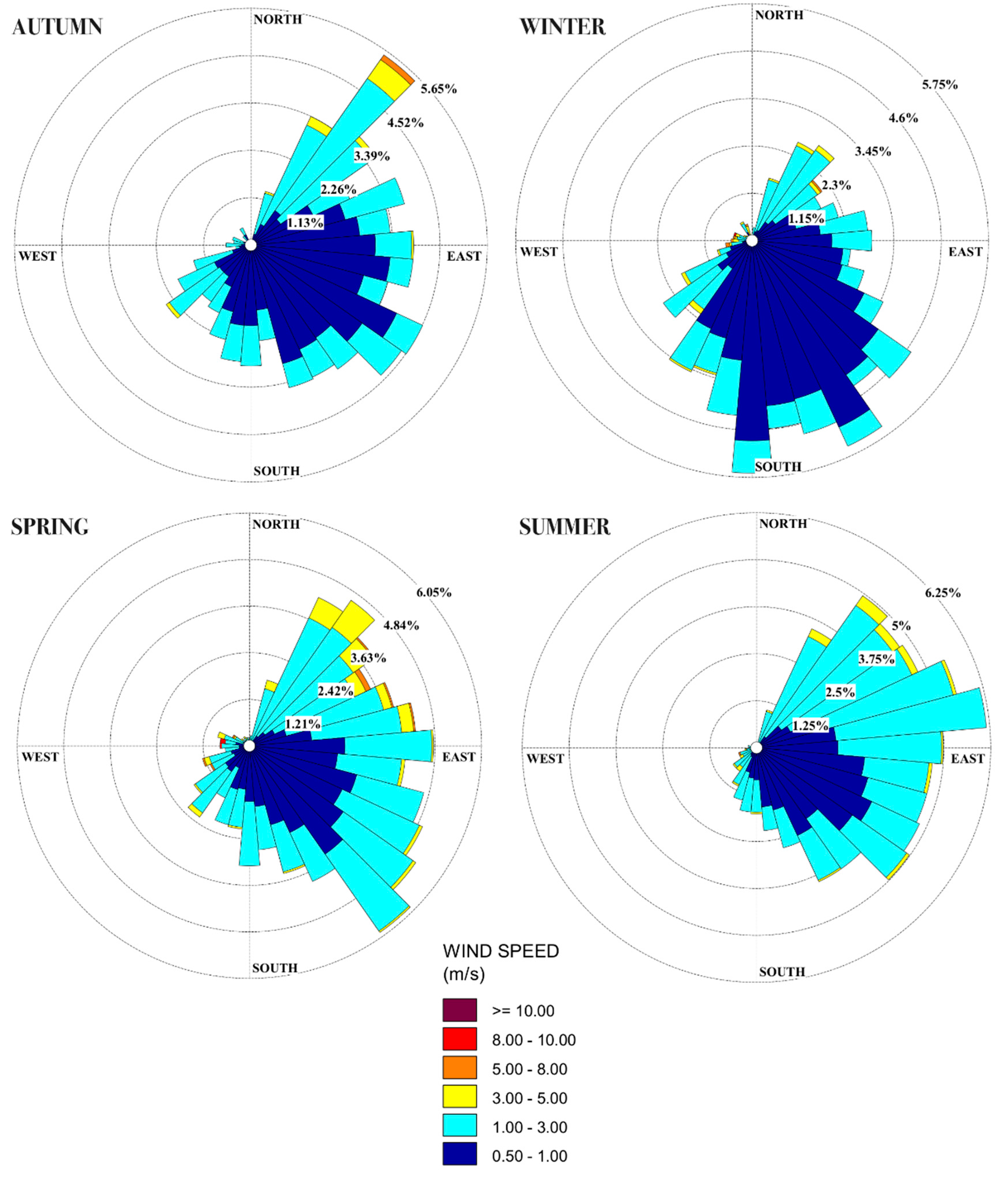
Table 1, Simulation 1 and Simulation 2 differed only in the weather input (2019 and 2018, respectively). Seasonal wind distributions of the two years are reported in
Figure 2 and
Figure 3. These figures show the typical wind distribution of this region, which is regulated by prevailing NE and SE directions. NE winds generally have higher speeds, especially in spring and autumn. However, low wind speeds (<3 m s
−1) have higher occurrence frequencies due to the presence of the Alps that surround the entire region, acting as a barrier for continental winds. A share of 29.8% and 22.4% of wind calms was registered for the years 2018 and 2019, respectively. Daily wind variations show that the evening and night hours registered the lowest intensities, with a morning increase and maximum values in the early afternoon. Even though wind distribution is similar in the two years, wind presence was higher in 2019 than in 2018. If the atmospheric stability class distribution is considered, in both years stable conditions prevailed (47%), followed by unstable (37%) and neutral conditions (16%). The Pasquill–Gifford atmospheric stability class distribution and wind directions for the years 2018 and 2019 are reported in
Figure 4 and
Figure 5, respectively. These figures also show a similar trend between the two years. In case of unstable conditions (Class A and B), NE is the prevailing wind direction, although the frequency of other directions is not negligible. This distribution reflects daytime conditions, where stability is mainly driven by thermal convection and higher-speed winds. Conversely, in case of stable conditions (Class E and F), SE is the prevailing wind direction. In this area of study, SE winds typically have a low speed (
Figure 3) and occur after sunset due to the balancing of the residual thermal energy between the valley and the surrounding reliefs. This latter situation of atmospheric stability and low winds may, in principle, favour the dispersion of odours to considerable distances.
The OERs were calculated following the methodology reported in
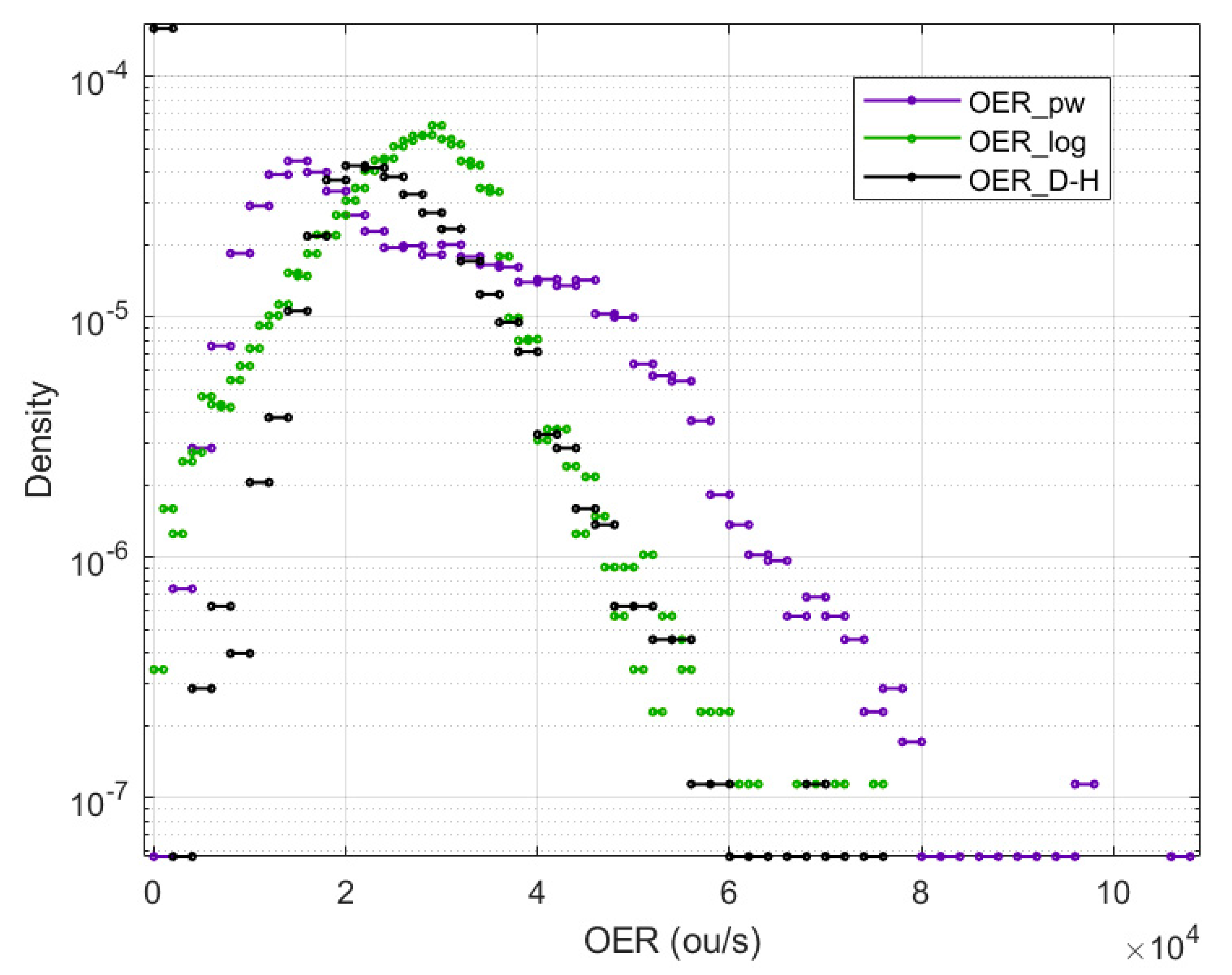
Section 2. Following Equation (5) (power law), Equation (6) (log law) and Equation (7) (D–H law), the hourly values of the OERs were obtained depending on the atmospheric conditions. To obtain a comparison, the hourly OERs were divided into classes, and their probability distributions were considered. In
Figure 6, the distribution of the OER of the primary settler (P3 in
Figure 1) is reported. Since
OERWT is constant for each source, the trend of a single source is also representative of other sources.
Figure 6 indicates how the OER changed depending on the correction method adopted. This comparison shows that the application of different wind speed correction methods (power law, log law and D–H law) provided different OER values. The distributions of both the power law and the log law indicate a peak density. For the power law, the most frequent value of the OER is around 15,000 OU/s. For the log law, the most frequent value of the OER is around 30,000 OU/s. The application of the D–H law provided two peak densities: the first is in correspondence of the values of the OER around zero, and the second is around 22,000 OU/s. For higher values of the OER, the distributions of the log and the D–H laws perform similarly. For the power law, the distribution is shifted towards higher OER values.
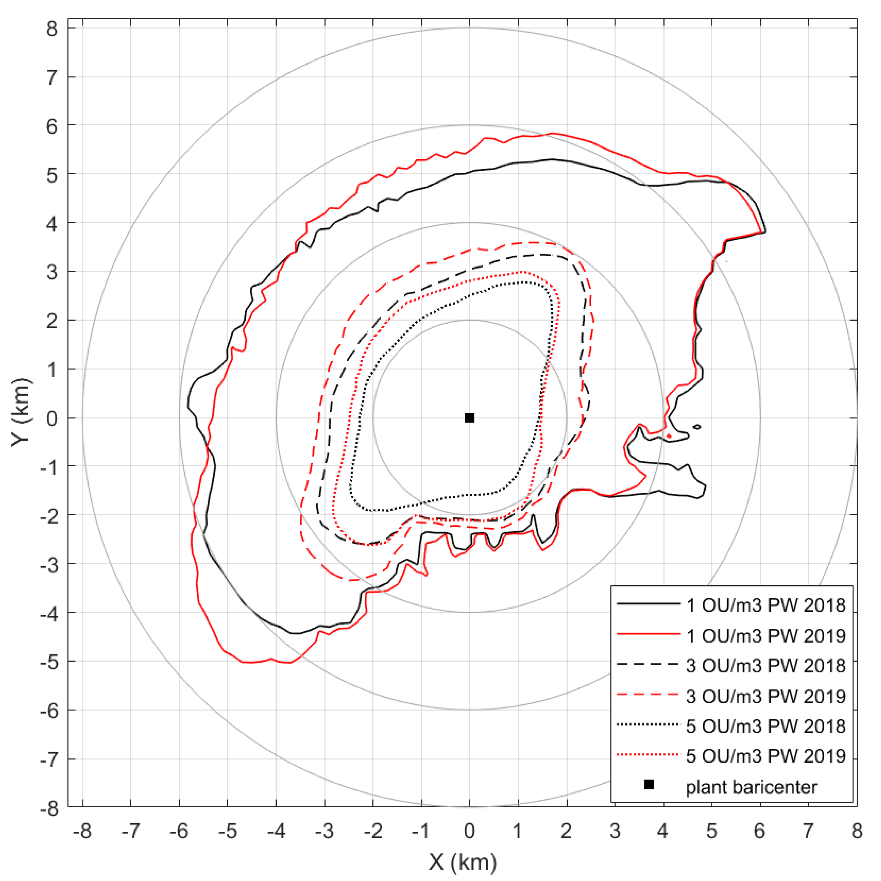
The separation distances corresponding to Simulation 1 (year 2019, power law) and Simulation 2 (year 2018, power law) for C
T equal to 1 OU m
−3, 3 OU m
−3 and 5 OU m
−3 are reported in
Figure 7. This figure shows that the odour impact area of the WWTP may be significant. The odour impact area is extended in the SW direction, in accordance with the anaemological data. Furthermore, the separation distances are higher in the NE direction, which is not fully in agreement with the prevailing wind directions reported. The 1 OU m
−3 isopleth reached towns up to 6 km away from the plant boundary, far beyond the 3 km limit set by the guidelines as a radius within which to verify the olfactory harassment extent. Contour lines referred to C
T = 3 OU m
−3 and C
T = 5 OU m
−3 (which indicate a greater frequency of harassment perception by the population) extend beyond the plant borders, including the nearby residential areas.
Figure 7 also shows the effect of the different meteorological data compared based on the same emission scenario. Contour lines show that the separation distances for the 1 OU m
−3 isopleths of the two years are similar, while some difference is reported for the 3 OU m
−3 and 5 OU m
−3 isopleths. Simulation 2 generated lower separation distances than Simulation 1. The shape of the impacted areas shows that the prevailing NE winds contribute to odour dispersion in the area. The contribution of SE winds is instead less evident. This graph also shows how the presence of the reliefs in the southern area contributes to limiting the odour dispersion in this direction. The maximum separation distances for C
T = 1 OU m
−3, C
T = 3 OU m
−3 and C
T = 5 OU m
−3, respectively, were
for simulation 17,000 m in direction NE; 4300 m in direction SW; 3510 in direction SW;
for simulation 26,870 m in direction NE; 3580 m in direction SW; 2680 in direction SW.
Taking Simulation 1 as the reference, the average difference on the eight main cardinal positions was −2%, −9% and −17% for CT = 1 OU m−3, CT = 3 OU m−3 and CT = 5 OU m−3, respectively. A maximum difference of −16% (SW direction), −20% (SW direction) and −32% (S direction) was found for the three values of CT.
The separation distances corresponding to Simulation 3 and Simulation 4, compared to Simulation 1, are reported in
Figure 8. This figure shows how the odour concentration changed by changing the correction method for wind speed in the OER calculation. The same meteorological data (year 2019) were used in Simulations 1, 3 and 4. As reported in
Figure 8, the application of the D–H law generated lower separation distances. Conversely, separation distances were higher in case the log law was applied. The maximum separation distances for C
T = 1 OU m
−3, C
T = 3 OU m
−3 and C
T = 5 OU m
−3, respectively, were
for simulation 37,800 m in direction NE; 4550 m in direction SW; 3720 in direction SW;
for simulation 46,500 m in direction SW; 4120 m in direction SW; 3300 in direction SW.
Taking Simulation 1 as a reference, the average variation of the separation distances on the eight main cardinal positions with the application of the log-law was +8%, +10% and +10% for C
T = 1 OU m
−3, C
T = 3 OU m
−3 and C
T = 5 OU m
−3, respectively. The average variation of the separation distances with the application of the D–H law was −7% for all values of C
T. A maximum difference of +19% (log law, SW direction), +25% (log law, NE direction) and +20% (log law, E direction) was found for the three values of C
T. In the S and SE directions, the difference between the three simulations is less visible. This is probably due to the presence of the topographic reliefs, which act as a barrier to odour dispersion. Increasing the level of C
T, the difference between the separation distances tended to be lower. Contour lines of C
T = 3 OU m
−3 also show a different shape in the ENE direction if the log law is applied. A further comparison of the separation distances in the main transport directions for the three applied relationships is reported in
Figure 9. This figure shows that the application of the log-law generally yields higher separation distances in all directions. Except for the E, SE and S directions, where the effect of the orography is evident, the difference maintains the proportionality D–H law < power law < log law.
4. Discussion
This study focused on the aspects of variability related to the application of regulatory OIC criteria to a WWTP located in Northern Italy. Two factors were investigated. The first factor was the use of different meteorology datasets as input to odour dispersion modelling. The second factor was the adoption of different correction methods for the wind speed profile used in the calculation of OERs.
Simulations 1 and 2 showed that the odour impact area is extended in the NE–SW direction, partially in accordance with the anaemological data.
Figure 7 showed that the extent of the distances was probably a combination of many factors, in particular the frequency distribution of atmospheric stability and wind speeds per wind direction sector. A similar trend was found by Brancher et al. [
11].
Compared to 2019, the year 2018 showed similar wind distribution patterns. The distribution and frequency of the atmospheric stability classes were also similar in the two years. As reported in
Figure 7, for C
T = 1 OU m
−3, the average difference in the resulting separation distances was around 7%. Conversely, for C
T = 3 OU m
−3 and mostly for C
T = 5 OU m
−3, an average 17% difference (maximum 32%) was reported. These variations may be attributed to the differences in wind distribution in the two years, which is more visible closer to the source. At higher distances, the results reflect the combined effect of the different factors that regulate odour dispersion (multiple wind components and convective turbulence in particular).
In another study, Brancher et al. [
9] analysed the variation of the separation distances over a 5-year meteorological dataset. For an OIC with a C
T = 1 OU m
−3, according to the present study, the results showed some inter-annual variability, especially in the main wind directions. The authors also found that, at the two investigated sites, the mean direction-dependent separation distances over the individual meteorological years were largely in agreement with the distances determined for the five years of meteorology data. They concluded that a one-year dataset of hourly meteorological observations is enough to be taken as a plausible length of time to attain reliable distances. Even though the present study is partly in agreement with these findings, the results show that, for higher values of C
T, higher inter-annual variability of separation distances could be expected.
The second aspect analysed in the present study showed that the application of different correction methods for wind speed calculation affects the resulting separation distances. Compared to the power law, the log law provides higher distances (8–10%), while the D–H law provides lower distances (7%). The variation is higher along with the prevailing wind directions. Maximum variations are recorded for the log law and can be up to 19%, 25% and 20% for C
T = 1 OU m
−3, C
T = 3 OU m
−3 and C
T = 5 OU m
−3, respectively. The results reflect the distribution of the OER values reported in
Figure 6. The reason for such a discrepancy must be investigated by analysing the form of Equations (5)–(7), which describe the wind speed correction. If the power law is applied (Equation (5)), the resulting value of the wind speed is highly dependent on the Hellman’s parameter (
α) assigned to each observation (
Table 4). Taking
h2 = 10 m and
h1 = 1 m, for stable conditions (
α = 0.07), a slight correction is applied, i.e., the corrected value
v1 is close to the value
v2 registered by the anemometer. Conversely, for unstable conditions (
α = 0.55), the value of
v2 is significantly reduced compared to
v1. If the log law is considered, the second term in Equation (6) represents the contribution of stability-induced turbulence. At the height h
1, the contribution of this term is generally low. This means that the term ln (
h1/
z0) is close to the value of
Kv; thus, the value of
v1 approximates the value of
u*. Considering that, at
h2, the
u*/
u ratio is close to unity; it comes out that the value of
v1 is close to
v2 in most cases. These aspects could be the main reasons for the differences in the OER values of
Figure 6 and, consequently, on the results of the separation distances reported in
Figure 8. Finally, if the D–H law is considered, Equation (7) shows that this relationship is regulated by the term H, which is the equilibrium boundary layer height. Equation (7) approximates to the log law when the term
h1/
H equals unity, i.e.,
H = 1. For low values of
u*, as in the present case study, the entire second term of Equation (7) tends to be null; thus, at the height
h1,
v2 reaches values close to zero. For this reason, the application of the D–H law resulted in a higher frequency of OER values close to zero (
Figure 6). This approach can be considered interesting and is worthy of further investigations as, in principle, it seems to provide an approximation of the wind speed conditions at lower heights that is closer to the real conditions, especially when the height of the source is close to the value of
z0.
Calculating the OER has been considered in previous studies. However, there are no studies in which the different OER calculation methods are matched to the dispersion modelling and compared in terms of separation distances. Previous works analysed (i) the correlation between emissive flows in the open field and within the dynamic hoods and (ii) the law used to describe the wind speed profile. Lucernoni [
30] addressed the issue of dependence on the velocity law by comparing the three correlations presented in this study, finding differences consistent with the results of this article. The same authors also underlined the greater reliability of the logarithmic profile for reduced elevations (0–100 m), while highlighting its complexity regarding application. Furthermore, they recognized the possibility of adopting the D–H relationship, citing it in a subsequent study concerning an OER correction of the passive area sources in Northern Italy [
18].
It must be pointed out that the present study was based on constant values of
OERWT. Odour emissions from WWTPs are known to fluctuate over time [
31,
32]. The use of time-varying OERs, however, is not yet easily feasible in odour modelling, as multiple monitoring campaigns are expensive in terms of time and costs. Repeating the investigation with alternative WWTP case studies and/or
OERWT values, e.g., those deriving from regulatory emission factors, could provide important information in the view of discussing the impact of different OIC on separation distances.
5. Conclusions
The objective of the present study was to investigate the variability of two factors (meteorology and OER calculation) related to the regulatory odour impact assessment, applying a modelling analysis to a wastewater treatment plant located in Northern Italy. The odour impact criteria of the Northern Italian regions were considered as the benchmark. Possible alternative technical choices were analysed to understand their influence on the resulting separation distances.
Regarding the influence of different meteorological years on the separation distances, this study was partially in agreement with the existing literature. For low odour concentration thresholds (CT = 1 OU m−3), the results showed that the two different years (2018 and 2019) provided similar patterns of the separation distances. The difference between the two years tended to increase by increasing the value of the concentration threshold (CT = 3 OU m−3 and CT = 5 OU m−3). Overall, differences in the separation distances were greater for the prevailing wind directions compared to non-prevailing wind directions.
The comparative analysis of the wind speed correction methods in the calculation of the OERs considered three different relationships: the power law, the logarithmic law and the Deaves–Harris law. The results showed that the OERs and separation distances varied depending on the selected method. Taking the power law as a reference, the average variability of the separation distances was between −7% (D–H correlation) and +10% (logarithmic law). Higher variability (up to 25%) was found for single transport distances. The main reason of such variability may be attributed to the different parameterization of the PBL of the three methods in relationship with the atmospheric stability class. From this study, it cannot be concluded if one method is more representative of another. However, it is highlighted that the application of the Deaves–Harris law is interesting but needs further investigation.
The present study confirmed that the representativeness of the odour impact assessment depends not only on the evaluator’s choices but also on the application of the current regulatory provisions on odour emissions. Populations and administrations are increasingly concerned with environmental odour problems. Although the odour impact criteria are the result of both technical and political considerations, it seems plausible that the different assessment methods should provide similar separation distances. The present study provided knowledge towards a better alignment of the concept of the odour impact criterion.


