Article

Quasi-Biennial Oscillation and Sudden Stratospheric Warmings during the Last Glacial Maximum

1
Department of Atmospheric Sciences, University of Washington, Seattle, WA 98195, USA
2
Department of Earth, Ocean and Atmospheric Sciences, University of British Columbia, Vancouver, BC V6T 1Z4, Canada
*
Author to whom correspondence should be addressed.
Atmosphere 2020, 11(9), 943; https://doi.org/10.3390/atmos11090943
Submission received: 6 August 2020 / Revised: 31 August 2020 / Accepted: 1 September 2020 / Published: 3 September 2020
(This article belongs to the Special Issue The Impacts of Climate Change on Atmospheric Circulations)

Abstract

:
The quasi-biennial oscillation (QBO) and sudden stratospheric warmings (SSWs) during the Last Glacial Maximum (LGM) are investigated in simulations using the Whole Atmosphere Community Climate Model version 6 (WACCM6). We find that the period of QBO, which is 27 months in the preindustrial and modern climate simulations, was 33 months in the LGM simulation using the proxy sea surface temperatures (SSTs) and 41 months using the model-based LGM SSTs. We show that the longer QBO period in the LGM is due to weaker wave forcing. The WACCM6 simulations of the LGM, preindustrial, and modern climates do not support previous modeling work that suggests that the QBO amplitude is smaller (larger) in a warmer (colder) climate. We find that SSWs in the LGM occurred later in the year, as compared to the preindustrial and modern climate, but that time of the final warming was similar. The difference in SSW frequency is inconclusive.

1. Introduction

The stratosphere during the Last Glacial Maximum (LGM) is expected to be considerably different than in the preindustrial and modern climate because of reduced CO2, CH4, and N2O concentrations; the presence of large ice sheets in the Northern Hemisphere (NH); and lower sea surface temperature (SST) [1,2,3]. Modeling studies show a slower Brewer-Dobson circulation (BDC) during the LGM than in the modern climate [4,5,6], which is consistent with model-projected BDC strengthening in response to greenhouse gas-induced warming [7,8,9,10,11,12,13,14]. The latter is supported by satellite observations [15,16]. Fu et al. [5] and Wang et al. [17] used the Whole Atmosphere Community Climate Model version 6 (WACCM6) [18] to examine the BDC and stratospheric O3 during the LGM. They showed that the stratospheric O3 changes in the LGM as compared to the preindustrial climate were caused by chemical processes in the upper stratosphere associated with a temperature increase and OH and NOx decreases, a slow-down of the BDC in the lower stratosphere, and a lowering of the tropopause in the extratropics [17]. In this study, we examine two aspects of stratospheric variability in the LGM—the quasi-biennial oscillation (QBO) and sudden stratospheric warmings (SSWs)—both with known links to the troposphere [19,20], by analyzing the same simulations described in Fu et al. [5] and Wang et al. [17].
The QBO is the primary mode of interannual variability in the tropical stratosphere, characterized by the downward propagating easterly and westerly wind regimes with an average period of ~28 months [21]. The model study of the QBO changes in a warming climate by Giorgetta and Doege [22] suggested a shorter QBO period at two times pre-industrial CO2 (2 × CO2) due to an increased gravity wave sources, while Kawatani et al. [23] and Watanabe and Kawatani [24] indicated a longer QBO period but weaker QBO amplitude in the warming climate simulations due to increased tropical upwelling. By analyzing global warming scenarios in the Coupled Model Intercomparison Project phase 5 (CMIP5) models that are capable of simulating QBO-like variability, Kawatani and Hamilton [25] found a long-term reduction in the QBO amplitude in the lower stratosphere but their results concerning QBO period changes were inconclusive. They also showed a QBO amplitude reduction at 70 hPa in observations from 1953 to 2012 but no significant trends in QBO period. Butchart et al. [26] examined 10 CMIP6 models with realistic QBO and found a weakening of the QBO in all 10 CMIP6 models and shortened QBO periods in 7 of the 10 models under warming scenarios. Richter et al. [19] examined the response of the QBO to a warming climate in eleven atmosphere general circulation models. No consistency was found among the models for the QBO period response, with the period decreasing by 8 months in some models and lengthening by up to 13 months in others in the 2 × CO2 simulations. In contrast, all the models projected a decrease in the QBO amplitude for 2 × CO2.
On the other hand, the SSW is a wintertime event in which the polar stratospheric temperature rises by several tens °C over the course of a few days and the stratospheric polar vortex reverses direction completely, with a subsequent recovery after the event [27]. SSWs occur about six times per decade in the NH [28]. SSWs can also occur in the Southern Hemisphere, but they are rare because of the small planetary wave amplitudes there [29], largely due to a lack of large-scale mountain ranges [30,31,32]. In this paper, we study only SSWs in the NH. The response of SSW frequency to increasing CO2 concentrations was investigated in several studies, but there is no consensus on changes in the number of SSWs [20,33,34,35,36,37,38]. For example, Bell et al. [36] showed that at four times pre-industrial CO2 (4 × CO2), the frequency of SSW events per year is doubled with respect to the control simulation. By analyzing the Coupled Model Intercomparison Project Phase 6 (CMIP6) simulations, Ayarzaguena et al. [20] found that there is a large disagreement across the models as to the sign in changes of SSW frequency under 4 × CO2 forcing, with some models showing the rate to be significantly halved and others showing it to be significantly doubled.
Herein, we analyze the LGM simulations that used the prescribed SST from both model simulation and proxy data, and compare them with results of pre-industrial and modern climate simulations that used the observed SST and sea ice. We find that the period of QBO increases from 27 months in the preindustrial and modern climate to 33–41 months in LGM, while the SSWs in the LGM are found to occur later in the year. We analyze simulations of the LGM and preindustrial and modern climate constrained by observed SSTs to help broaden our perspective regarding the stratospheric response to anthropogenically induced climate changes in the future.

2. Model Experiments

The WACCM6 has a realistic, internally generated QBO in the stratosphere and simulates a realistic frequency of SSWs [18,39]. We analyzed five simulations from Fu et al. [5] and Wang et al. [17], who used the WACCM6 with a horizontal resolution of 0.9° latitude and 1.25° longitude and 70 vertical levels. They consist of (1) a LGM simulation with prescribed SSTs based on models (LGMPMIP3), (2) a LGM simulation with SSTs based on proxy data (LGMPROXY), (3) a preindustrial climate simulation (PI), (4) a modern climate simulation (MC), and (5) a modern climate simulation without ozone-depleting substances (ODS) (MCno_ODS). Each simulation was 60 years long, and only the last 50 years were analyzed. For the PI (MC and MCno_ODS) simulations, the SSTs and sea ice were the observed climatology of 1870–1890 (1980–2000) with a seasonal evolution [40]. For LGMPMIP3, the SSTs and sea ice data were obtained as the model differences between multi-model mean SST and sea ice for the LGM from PMIP3 [41] and the corresponding modern climate simulation plus the modern observed SSTs and sea ice. For LGMPROXY, the SSTs were from the MARGO proxy data [42]. The simulations from LGMPMIP3 and LGMPROXY provide information on the sensitivity of results to the SSTs used for the LGM. In the LGM simulations, the WACCM6 was coupled to the CLM4.0 LGM land boundary conditions [43] with the ice sheet topography from Abe-Ouchi et al. [44]. The greenhouse gas concentrations and orbital parameters corresponding to the LGM, preindustrial, and modern climate were used [5,17]. The ozone depletion substances (ODSs) in MC were taken from the year 2000.

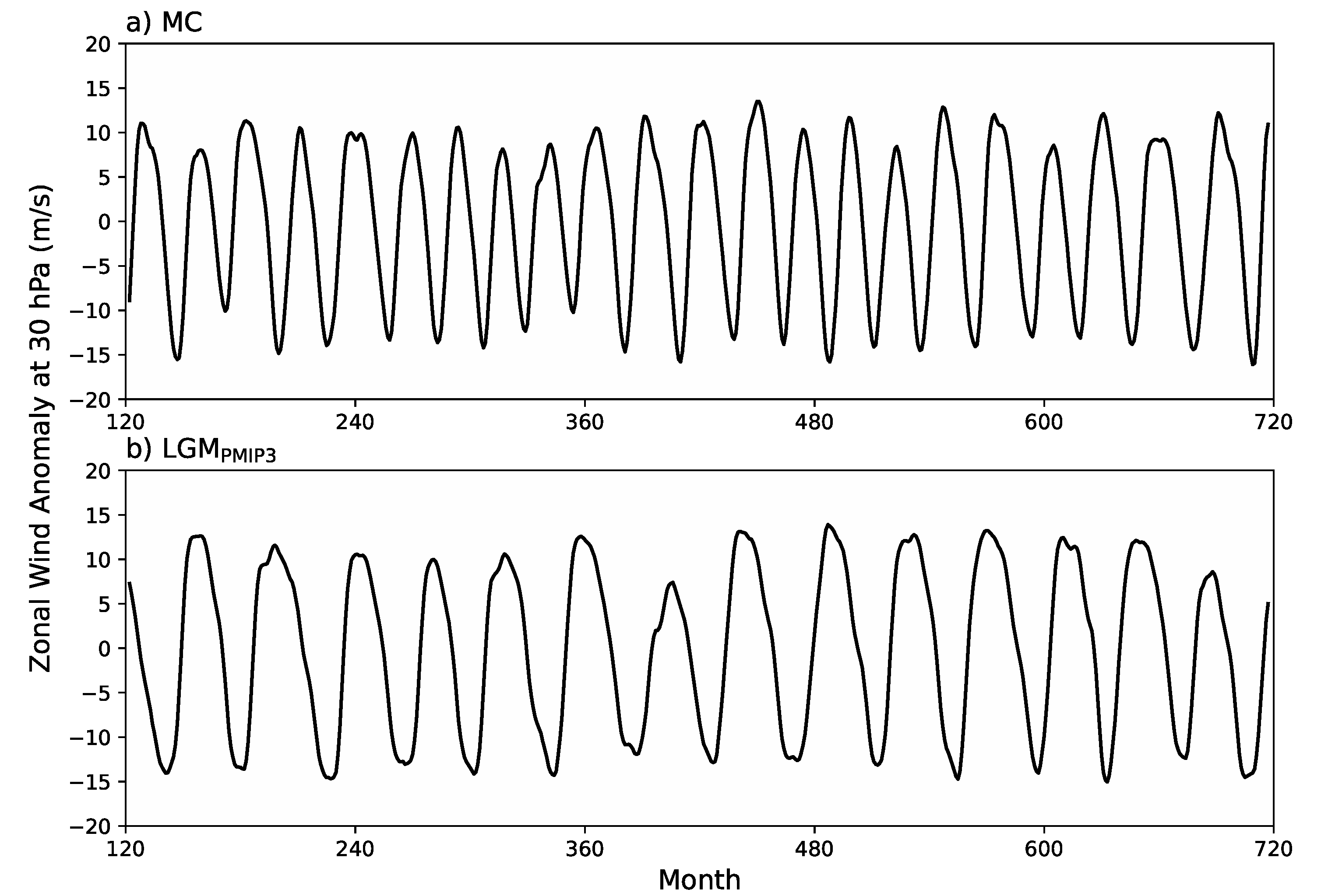
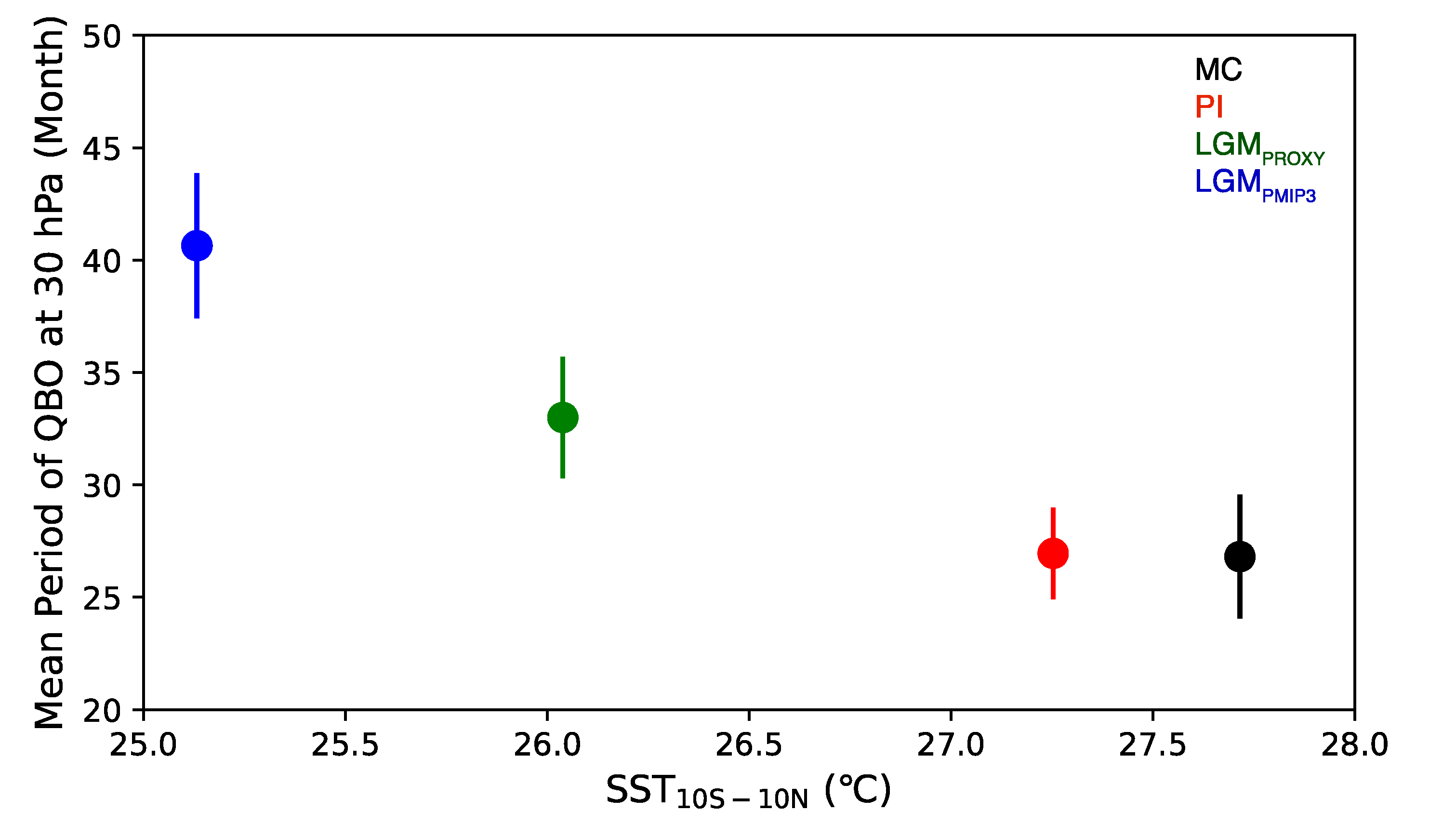
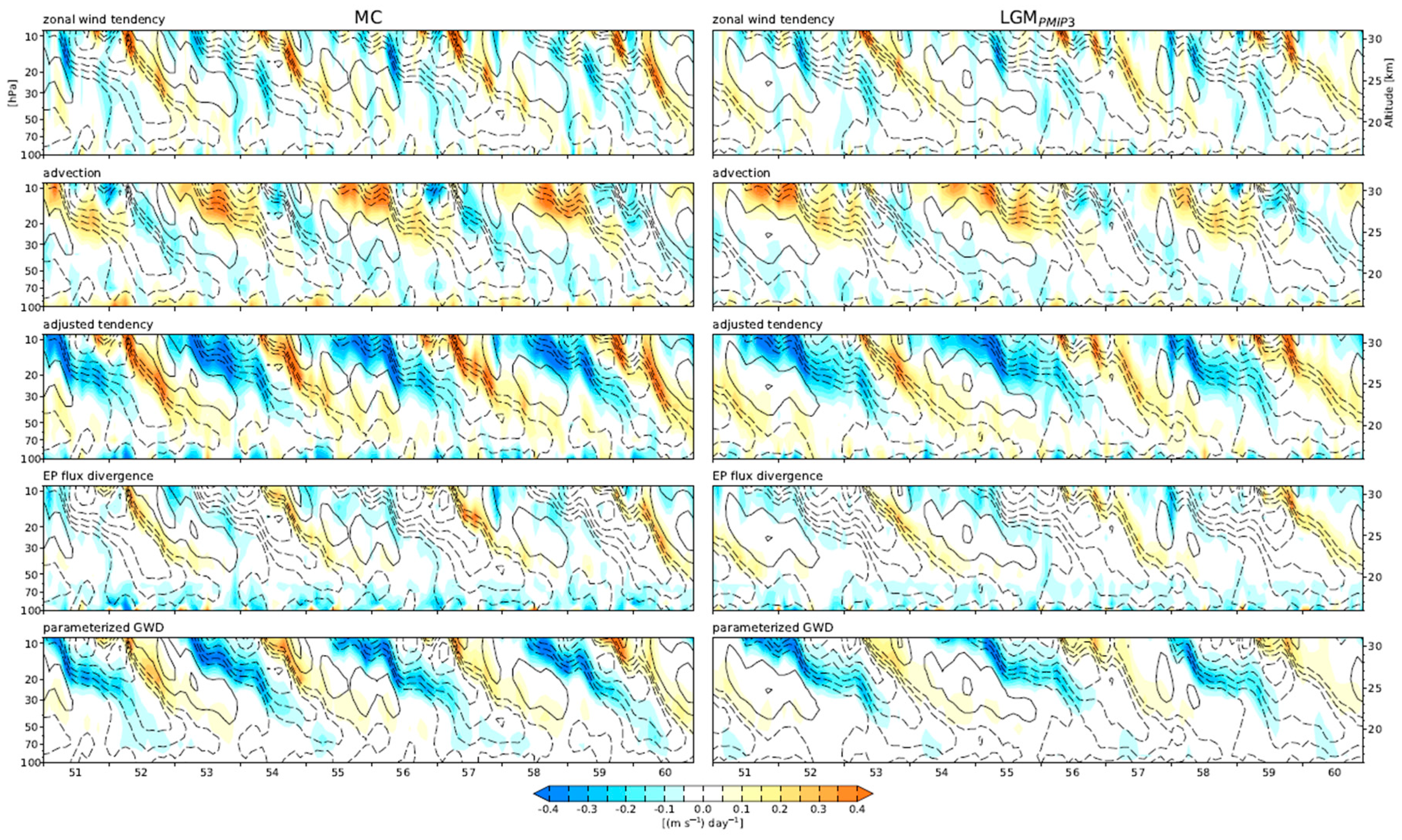
3. The QBO in the LGM

Figure 1 shows the deseasonalized monthly time series of the zonal-mean zonal wind averaged over 5° S–5° N at 30 hPa for MC and LGMPMIP3, which suggests a substantial increase in the QBO period during the LGM. Here, we define the QBO cycle with the transition time method that identifies zero wind transitions from easterly to westerly winds [19,45]. We use the zonal-mean zonal wind monthly anomaly time series averaged over 5° N/S, smoothed using a five-month centered running mean, e.g., as in Richter et al. [19]. The period and amplitude for each QBO cycle between individual transition points is defined, and the mean and standard deviation of the periods and amplitudes can then be derived. The QBO mean periods for MC, PI, LGMPROXY, and LGMPMIP3 are about 27, 27, 33, and 41 months, respectively, at both 10 and 30 hPa (Table 1), and are found to be independent of the altitude (Figure 2a). The mean periods of WACCM6-simulated QBO in the MC and PI agree well with observations [21]. The mean QBO periods for LGMPROXY and LGMPMIP3 are about 6 and 14 months longer, respectively, than in MC (Table 1 and Figure 2a). The differences in the QBO period between LGMPMIP3 and MC, LGMPROXY and MC, and LGMPMIP3 and LGMPROXY are all statistically significant at the 95% confidence level.
The global-mean surface air temperatures are 15.0, 10.6, and 10.1 °C for the MC, LGMPROXY, and LGMPMIP3, respectively, corresponding to global-mean SSTs of 18.4, 16.6, and 16.2 °C (Table 1). The global-mean surface air temperatures and SSTs from LGM PMIP3 are thus only ~0.4–0.5 °C lower than LGMPROXY. However, the SSTs averaged over 10° S–10° N, which are more relevant to QBO, are 27.7, 26.0, and 25.1 °C for MC, LGMPROXY, and LGMPMIP3, respectively (Table 1). The SST over the deep tropics for LGMPMIP3 is thus 0.91 °C lower than LGMPROXY. Figure 3 shows the mean QBO periods versus SST averaged over 10° S–10° N, indicating an increase in the QBO period with a decrease in SSTs over the deep tropics.
Figure 4 shows time-height sections of zonal-mean zonal wind tendency and the contributions from different terms in the zonal-mean zonal momentum budget (colored shading), averaged over 5° S–5° N, for the last 10 years of the (left) MC and (right) LGMPMIP3 simulations. Also shown is the zonal-mean zonal wind distribution (coutours). Similar results are obtained for LGMPROXY (not shown).
It is evident from Figure 4 that the zonal wind tendency (i.e., the time derivative of the zonal-mean zonal wind) (1st row) is generally smaller in LGM than in MC. The advection (2nd row) is due to the residual mean meridional circualtion and is dominated by the near-equatorial vertical advection (not shown). The advection tends to damp the zonal wind pertaurbation in the QBO, especially during the descent of the easterly shear zones, consistent with the observations [46]. The damping by the advection is weaker in LGM, as is the upward BDC [5], which opposes the downward propagation of successive easterly and westerly phases of the QBO. The adjusted tendency (3rd row) is the zonal wind tendency minus advection, which is the zonal wind tendency that remains to be explained by the wave forcing associated with the Eliassen-Palm (EP) flux divergence (i.e., the resolved wave forcing) (4th row) and the parameterized gravity wave drag (GWD) (5th row). The adjusted tendency is appreciably smaller in LGM, indicating a smaller wave forcing at that time. The EP flux divergence is considerably stronger in the westerly shear zones than that in the easterly shear zones. This is because the QBO eastward forcing is mainly due to planetary-scale Kelvin waves, while its westward forcing is dominated by gravity waves [47]. WACCM6 with its limited horizontal and vertical resolutions is not capable of resolving the gravity waves, which must be parameterized. It is evident from Figure 4 that the parameterized GWD dominates the wave forcing in both MC and LGM simulations, especially during the descent of the easterly shear zones. Both resolved wave forcing and parameterized GWD are smaller in LGM than their counterparts in MC (Figure 4). The weaker resolved wave forcing in LGM could be attributed to weaker wave activity and/or weaker shear zones in LGM. The latter can be interpreted as a result of similar QBO amplitudes in LGM and MC (Figure 2) but a longer QBO period in LGM. The weaker parameterized GWD in the LGM reflects the smaller latent heat release associated with weaker convection over colder tropical oceans.
It is suggested that the QBO period in the LGM from the WACCM6 simulations is longer than in the MC, because the wave forcings over both westerly and easterly shear zones are weaker (Figure 4). The result is that it takes longer for the QBO to be forced from one phase to another in the LGM, although the weakening of the BDC partly cancels the wave forcing effects.
Previous studies have suggested that a QBO period increase results from a decrease of wave sources and/or an increase in tropical upwelling [19,22,23,24,48]. Richter et al. [19] indicated that changes in the gravity wave momentum flux entering the stratosphere has a stronger influence on the QBO period than the tropical upwelling changes. In view of the weaker tropical upwelling in the LGM relative to MC [5], the weaker wave fluxes must be mainly responsible for the longer period (Figure 4). In the models considered by Richter et al. [19], vertical advection and the resolved wave forcing did not play a large role in driving the QBO period changes in a warming climate: the change was mainly due to parameterized momentum flux due to gravity wave entering the stratosphere from below. Figure 4 suggests that the gravity wave forcing associated with cold climate was indeed smaller. That the QBO period was longer in the cold (LGM) climate simulated by the WACCM6 is consistent with the shorter period in the warmer climate simulated by WACCM5 [19].
Now, let us consider the change in QBO amplitude from LGM to MC. Following [19], we define QBO amplitude using the transition time method in which the amplitude for each cycle is estimated as the difference between the maximum and minimum zonal winds divided by two. The mean QBO amplitude is also estimated following Dunkerton and Delisi [49] as 2 σ, where σ is the standard deviation of the deseasonalized time series of the monthly mean winds with 5-month running mean. The mean QBO amplitudes from the two methods are similar (Table 1 and Figure 2b,c). The differences between the QBO amplitudes estimated by comparing PI, LGMPROXY and LGMPMIP3 with MC are 9.0% (0.6%), −5.0% (−6.9%), and 4.1% (−2.3%), at 30 (10) hPa based on the transition time method. From Figure 2b,c, the QBO amplitude for PI (red lines) is larger than MC (black line), consistent with Butchart et al. [26] and Richter et al. [19] who showed a robust and systematic decrease in the QBO amplitude with increasing SSTs and CO2 concentration. However, the QBO amplitude for LGMPROXY (green lines) is smallest among the five simulations, while the QBO amplitude for LGMPMIP3 (blue lines) is larger than MC (black lines) but generally smaller than PI. Thus, the WACCM6 simulations of the LGM and preindustrial and modern climate do not support the notion that the QBO amplitude is smaller (larger) in warmer (colder) climate. The latter is shown by Butchart et al. [26] and Richter et al. [19] for a projected warming world from models including the WACCM5 and 6. One key difference between this study and Butchart et al. [26] and Richter et al. [19] is that we focus on the past and modern climate with the simulations constrained by observed SSTs. It is interesting to note that the amplitude differences between LGMPMIP3 and LGPPROXY and between PI and MC at 30 hPa are both statistically significant.
The QBO period and amplitude from MCno_ODS are very similar to those from MC (not shown). We also examined the QBO periods and amplitudes from all five simulations using the actual zonal wind instead of the zonal wind after removing the seasonal cycle. The results (not shown) are similar. One advantage of using the zonal wind monthly anomaly is that the QBO period can still be derived between 70 hPa and 50 hPa, where the QBO amplitude is largely underestimated by the models [45].
The QBO is largely driven and maintained by momentum deposition from upward propagating Kelvin waves, mixed Rossby-gravity waves, and gravity waves, but damped by vertical advection. Large-scale Kelvin and mixed Rossby-gravity waves in GCMs are generated largely by parametrized convections, and gravity wave parametrizations are tuned to obtain the present-day QBO period and amplitude, which constitute a large source of uncertainty in modelling of the QBO [19]. Thus, the LGM QBO from the WACCM6 might be model-dependent. Hence, it would be useful to be able to compare the WACCM results with those of other models.

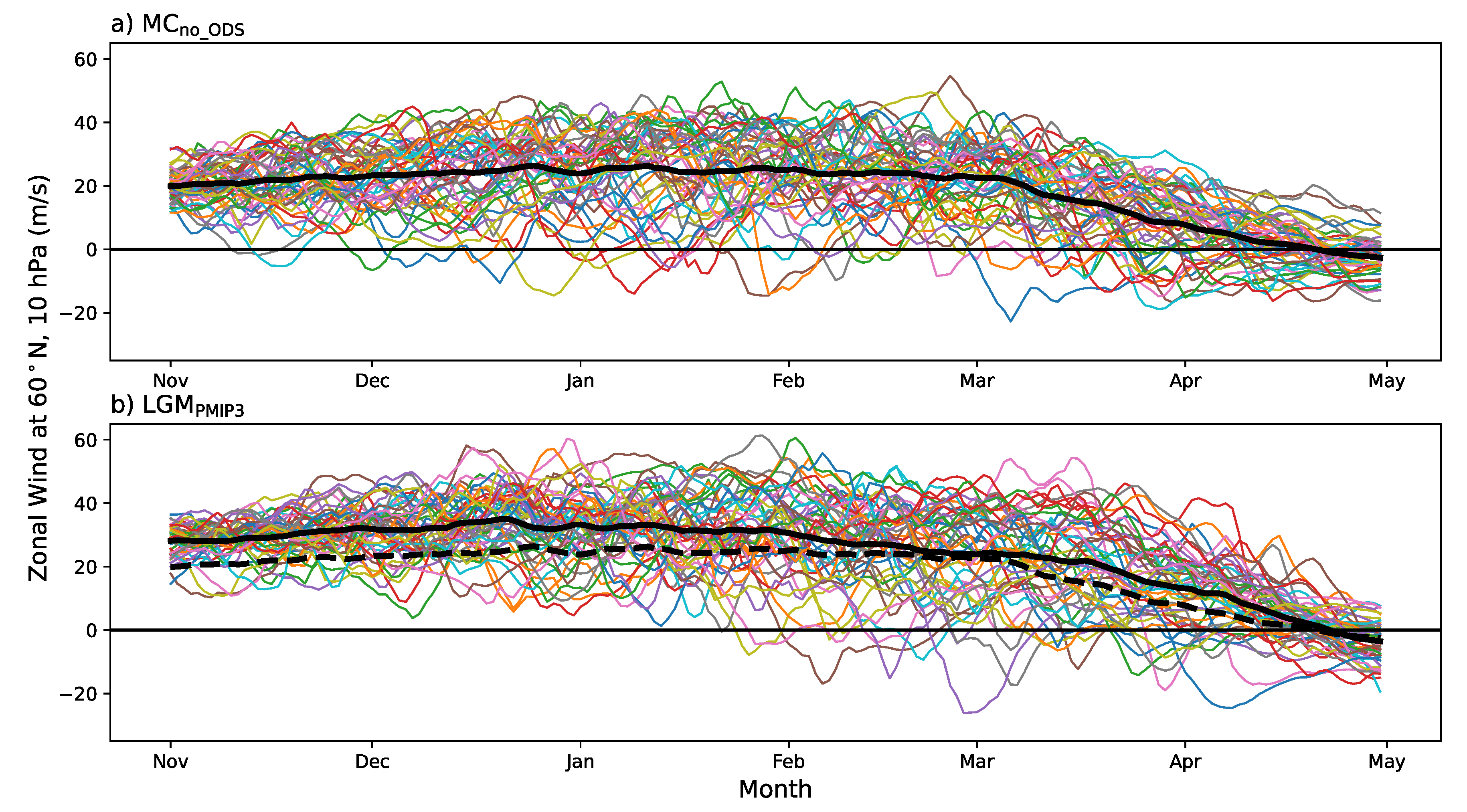
4. The SSWs in the LGM

We identify SSW events following Cao et al. [50] based on zonal-mean zonal wind as follows. The day on which the zonal-mean zonal wind at 60° N and 10 hPa turns from westerly winds to easterly winds, with easterly winds consequently lasting for more than five days, is defined here as the zeroth day of a sudden warming event. No new SSW events will be defined again during the 20 consecutive days following a prior SSW event. Stratospheric final warmings are excluded because the easterly winds persist until the next winter.
Figure 5 shows the daily time series of the zonal-mean zonal wind at 60° N and 10 hPa from November to May for each year of the simulations (50 thin color lines) along with the 50-year average (black thick line) for (a) MCno_ODS and (b) LGMPMIP3. The results from MC and LGMPROXY are similar (not shown). We see the larger mean westerlies during the LGMPMIP3 than in MCno_ODS by comparing black thick solid and dashed lines in Figure 5b. This is consistent with the weaker wave drag but stronger zonal winds in the stratosphere over the NH mid and high latitudes in the winter (Figure 6b,c). Note that positive change (Figure 6c) in the negative wave drag regions is indicative of a smaller absolute wave drag. While lower greenhouse concentrations during the LGM favor a warming of the stratosphere, the reduced warming in the upper stratosphere and even the cooling in the lower stratosphere over the NH high latitudes almost certainly reflect a dynamical cooling signal (Figure 6a). This dynamical cooling in the cold climate is consistent with the previous modeling studies showing a boreal polar stratospheric dynamic warming in the warming world due to increasing CO2 [33,51]. Note that for the MC including ODS, the stratospheric temperature change is not only caused by the changes in greenhouse gas concentrations and wave activities but also by the anthropogenic O3 depletion. In this case, the dynamic signature in the temperature fields is not obvious because wave and O3 effects have an opposite sign (not shown). Since the ozone depletion impact on the SSWs is not the purpose of the paper, we only show the comparison between LGM and MCno_ODS in Figure 6.
Figure 5 shows that the episodes of easterlies associated with SSW events tend to occur later in the year during the LGMPMIP3 than MCno_ODS. The first SSW event appears in November for both MCno_ODS and MC, December for PI, and January for both LGMPROXY and LGMPMIP3 (Table 2). However, a similar mean final warming day between day 115 to day 119 (i.e., April 25 to April 29) is seen in all the five simulations (Table 2).
The SSW frequency is 0.66, 0.48, 0.38, 0.4, and 0.42 per year for MCno_ODS, MC, PI, LGMPROXY and LGMPMIP3, respectively (Table 2). In the MC, the ODSs were taken from the year 2000 when the ODSs were highest, which leads to the largest O3 depletion [52]. The average SSW frequency of MCno_ODS and MC, which is 0.57 per year, agrees well with observations [27,28]. The similarity of the SSW frequencies in PI, LGMPROXY and LGMPMIP3 (Table 2) is intriguing: is the lack of response in LGM because of countering influences from colder temperatures (fewer SSWs) but potentially more wave forcing from the ice sheet (more SSWs)? Table 2 also indicates that ozone depletion might reduce SSW frequency. Is this because the enhanced stratospheric cooling caused by the ozone depletion over the NH high latitudes leads to a stronger stratospheric zonal wind and thus it is harder to hit the 0 m s−1 threshold? In addition, is the difference in SSW frequency between PI and MCno_ODS (or MC) expected? Note that the significant test following Charlton et al. [53] shows that the SSW frequency difference between any two simulations is not statistically significant based on the 50 years simulations. We will examine these issues in our follow-up study by extending our simulations for a longer period of time and carrying out an additional LGM experiment by excluding the ice sheet.

5. Conclusions

The QBO and SSW during the LGM are examined in simulations using the WACCM6. It is found that the period of QBO, which is 27 months in the preindustrial and modern climates, was 33–41 months in LGM. The magnitude of the decrease in QBO period from then to now is sensitive to the SST over the deep tropics (10° S–10° N) prescribed in the LGM simulations. It is shown that both resolved wave forcing and parameterized GWD became smaller in LGM than those in MC from the WACCM6 simulations, leading to a longer QBO period despite a weaker advection in the LGM. The WACCM6 simulations of the LGM and preindustrial and modern climate do not support the notion that the QBO amplitude is smaller (larger) in warmer (colder) climate. It is shown that SSW events typically start to occur in January for the LGM but in November for the modern climate, but that the timings of the final warmings in the LGM and modern climate are similar. The similarity of the SSW frequencies in PI, LGMPROXY and LGMPMIP3 suggests potentially countering influences from colder temperatures and wave forcing associated with the ice sheet, which will be investigated in a follow-up study. Considering the past climate in our study helps to broaden our perspective regarding how the climate of the stratosphere may change in the future in response to human activities.

Author Contributions

Conceptualization, Q.F.; methodology, Q.F.; software, M.W., R.H.W. and H.A.P.; validation, Q.F. and J.M.W.; formal analysis, M.W. and H.A.P.; investigation, Q.F., M.W., R.H.W., H.A.P., B.A. and J.M.W.; resources, Q.F.; data curation, M.W. and R.H.W.; writing—original draft preparation, Q.F.; writing—review and editing, Q.F., M.W., R.H.W., H.A.P., B.A., J.M.W.; visualization, M.W. and H.A.P.; supervision, Q.F.; project administration, Q.F. and B.A.; funding acquisition, Q.F. and B.A. All authors have read and agreed to the published version of the manuscript.

Funding

This research was supported by National Science Foundation Grant AGS-1821437 and NASA Grant 80NSSC18K1031.

Acknowledgments

This research was supported by National Science Foundation Grant AGS-1821437 and NASA Grant 80NSSC18K1031. R.H.W. was partially funded by the European Union’s Horizon 2020 research and innovation program under the Marie Sklodowska-Curie Grant Agreement No. 797961. We thank George Kiladis for useful discussions. We would like to acknowledge high-performance computing support from Cheyenne (doi:10.5065/D6RX99HX) provided by NCAR’s Computational and Information Systems Laboratory, sponsored by the National Science Foundation, for the WACCM6 simulations and analyses presented in this study and for data management, storage, and preservation.

Conflicts of Interest

The authors declare no conflict of interest.

References

  1. Rind, D.; Chandler, M.; Lonergan, P.; Lerner, J. Climate change and the middle atmosphere 5. Paleostratosphere in cold and warm climates. J. Geophys. Res-Atmos. 2001, 106, 20195–20212. [Google Scholar] [CrossRef]
  2. Rind, D.; Lerner, J.; McLinden, C.; Perlwitz, J. Stratospheric ozone during the Last Glacial Maximum. Geophys. Res. Lett. 2009, 36. [Google Scholar] [CrossRef] [Green Version]
  3. Hu, Y.Y.; Xia, Y.; Liu, Z.Y.; Wang, Y.C.; Lu, Z.Y.; Wang, T. Distorted Pacific-North American teleconnection at the Last Glacial Maximum. Clim. Past. 2020, 16, 199–209. [Google Scholar] [CrossRef] [Green Version]
  4. Murray, L.T.; Mickley, L.J.; Kaplan, J.O.; Sofen, E.D.; Pfeiffer, M.; Alexander, B. Factors controlling variability in the oxidative capacity of the troposphere since the Last Glacial Maximum. Atmos. Chem. Phys. 2014, 14, 3589–3622. [Google Scholar] [CrossRef] [Green Version]
  5. Fu, Q.; White, R.H.; Wang, M.; Alexander, B.; Solomon, S.; Gettelman, A.; DBattisti, D.S.; Lin, P. The Brewer-Dobson Circulation during the Last Glacial Maximum. Geophys. Res. Lett. 2020, 47, e2019GL086271. [Google Scholar] [CrossRef] [Green Version]
  6. Noda, S.; Kodera, K.; Adachi, Y.; Deushi, M.; Kitoh, A.; Mizuta, R.; Murakami, S.; Yoshida, K.; Yoden, S. Mitigation of global cooling by stratospheric chemistry feedbacks in a simulation of the Last Glacial Maximum. J. Geophys. Res. Atmos. 2018, 123, 9378–9390. [Google Scholar] [CrossRef]
  7. Bunzel, F.; Schmidt, H. The Brewer-Dobson Circulation in a Changing Climate: Impact of the Model Configuration. J. Atmos. Sci. 2013, 70, 1437–1455. [Google Scholar] [CrossRef] [Green Version]
  8. Butchart, N.; Scaife, A.; Bourqui, M.; De Grandpré, J.; Hare, S.; Kettleborough, J.; Langematz, U.; Manzini, E.; Sassi, F.; Shibata, K. Simulations of anthropogenic change in the strength of the Brewer–Dobson circulation. Clim. Dynam. 2006, 27, 727–741. [Google Scholar] [CrossRef]
  9. Garcia, R.R.; Randel, W.J. Acceleration of the Brewer-Dobson circulation due to increases in greenhouse gases. J. Atmos. Sci. 2008, 65, 2731–2739. [Google Scholar] [CrossRef]
  10. Li, F.; Austin, J.; Wilson, J. The strength of the Brewer-Dobson circulation in a changing climate: Coupled chemistry-climate model simulations. J. Clim. 2008, 21, 40–57. [Google Scholar] [CrossRef]
  11. Lin, P.; Fu, Q. Changes in various branches of the Brewer-Dobson circulation from an ensemble of chemistry climate models. J. Geophys. Res-Atmos. 2013, 118, 73–84. [Google Scholar] [CrossRef]
  12. McLandress, C.; Shepherd, T.G. Simulated Anthropogenic Changes in the Brewer-Dobson Circulation, Including Its Extension to High Latitudes. J. Clim. 2009, 22, 1516–1540. [Google Scholar] [CrossRef]
  13. Oberlander, S.; Langematz, U.; Meul, S. Unraveling impact factors for future changes in the Brewer-Dobson circulation. J. Geophys. Res-Atmos. 2013, 118, 10296–10312. [Google Scholar] [CrossRef]
  14. Okamoto, K.; Sato, K.; Akiyoshi, H. A study on the formation and trend of the Brewer-Dobson circulation. J. Geophys. Res. Atmos. 2011, 116. [Google Scholar] [CrossRef] [Green Version]
  15. Fu, Q.; Lin, P.; Solomon, S.; Hartmann, D.L. Observational evidence of strengthening of the Brewer-Dobson circulation since 1980. J. Geophys. Res-Atmos. 2015, 120, 10214–10228. [Google Scholar] [CrossRef] [Green Version]
  16. Fu, Q.; Solomon, S.; Pahlavan, H.A.; Lin, P. Observed changes in Brewer–Dobson circulation for 1980–2018. Environ. Res. Lett. 2019, 14, 114026. [Google Scholar] [CrossRef] [Green Version]
  17. Wang, M.C.; Fu, Q.; Solomon, S.; White, R.H.; Alexander, B. Stratospheric Ozone in the Last Glacial Maximum. J. Geophys. Res. Atmos. 2020. accepted subject to minor revision. [Google Scholar]
  18. Gettelman, A.; Mills, M.J.; Kinnison, D.E.; Garcia, R.R.; Smith, A.K.; Marsh, D.R.; Tilmes, S.; Vitt, F.; Bardeen, C.G.; McInerny, J.; et al. The Whole Atmosphere Community Climate Model Version 6 (WACCM6). J. Geophys. Res. Atmos. 2019. [Google Scholar] [CrossRef] [Green Version]
  19. Richter, J.H.; Butchart, N.; Kawatani, Y.; Bushell, A.C.; Holt, L.; Serva, F.; Anstey, J.; Simpson, I.R.; Osprey, S.; Hamilton, K.; et al. Response of the Quasi-Biennial Oscillation to a warming climate in global climate models. Q. J. Roy. Meteor. Soc. 2020. [Google Scholar] [CrossRef]
  20. Ayarzaguena, B.; Charlton-Perez, A.J.; Butler, A.H.; Hitchcock, P.; Simpson, I.R.; Polvani, L.M.; Butchart, N.; Gerber, E.P.; Gray, L.; Hassler, B.; et al. Uncertainty in the Response of Sudden Stratospheric Warmings and Stratosphere-Troposphere Coupling to Quadrupled CO2 Concentrations in CMIP6 Models. J. Geophys. Res. Atmos. 2020, 125. [Google Scholar] [CrossRef]
  21. Baldwin, M.P.; Gray, L.J.; Dunkerton, T.J.; Hamilton, K.; Haynes, P.H.; Randel, W.J.; Holton, J.R.; Alexander, M.J.; Hirota, I.; Horinouchi, T.; et al. The quasi-biennial oscillation. Rev. Geophys. 2001, 39, 179–229. [Google Scholar] [CrossRef]
  22. Giorgetta, M.A.; Doege, M.C. Sensitivity of the quasi-biennial oscillation to CO2 doubling. Geophys. Res. Lett. 2005, 32. [Google Scholar] [CrossRef]
  23. Kawatani, Y.; Hamilton, K.; Watanabe, S. The Quasi-Biennial Oscillation in a Double CO2 Climate. J. Atmos. Sci. 2011, 68, 265–283. [Google Scholar] [CrossRef]
  24. Watanabe, S.; Kawatani, Y. Sensitivity of the QBO to Mean Tropical Upwelling under a Changing Climate Simulated with an Earth System Model. J. Meteorol. Soc. Jpn. 2012, 90A, 351–360. [Google Scholar] [CrossRef] [Green Version]
  25. Kawatani, Y.; Hamilton, K. Weakened stratospheric quasibiennial oscillation driven by increased tropical mean upwelling. Nature 2013, 497, 478–481. [Google Scholar] [CrossRef] [PubMed]
  26. Butchart, N.; Anstey, J.A.; Kawatani, Y.; Osprey, S.M.; Richter, J.H.; Wu, T. QBO changes in CMIP6 climate projections. Geophys. Res. Lett. 2020, 47, e2019GL086903. [Google Scholar] [CrossRef] [Green Version]
  27. Butler, A.H.; Sjoberg, J.P.; Seidel, D.J.; Rosenlof, K.H. A sudden stratospheric warming compendium. Earth. Syst. Sci. Data. 2017, 9, 63–76. [Google Scholar] [CrossRef] [Green Version]
  28. Charlton, A.J.; Polvani, L.M. A new look at stratospheric sudden warmings. Part I: Climatology and modeling benchmarks. J. Clim. 2007, 20, 449–469. [Google Scholar] [CrossRef]
  29. van Loon, H.; Jenne, R.L.; Labitzke, K. Zonal harmonic standing waves. J. Geophys. Res. 1973, 78, 4463–4471. [Google Scholar] [CrossRef]
  30. Yoden, S. An illustrative model of seasonal and interannual variations of the stratospheric circulation. J. Atmos. Sci. 1990, 47, 1845–1853. [Google Scholar] [CrossRef] [Green Version]
  31. Taguchi, M.; Yoden, S. Internal interannual variability of the troposphere-stratosphere coupled system in a simple global circulation model. Part I: Parameter sweep experiment. J. Atmos. Sci. 2002, 59, 3021–3036. [Google Scholar] [CrossRef]
  32. White, R.H.; Battisti, D.S.; Sheshadri, A. Orography and the Boreal Winter Stratosphere: The Importance of the Mongolian Mountains. Geophys. Res. Lett. 2018, 45, 2088–2096. [Google Scholar] [CrossRef]
  33. Rind, D.; Shindell, D.; Lonergan, P.; Balachandran, N.K. Climate change and the middle atmosphere. Part III: The doubled CO2 climate revisited. J. Clim. 1998, 11, 876–894. [Google Scholar] [CrossRef]
  34. Charlton-Perez, A.J.; Polvani, L.M.; Austin, J.; Li, F. The frequency and dynamics of stratospheric sudden warmings in the 21st century. J. Geophys. Res. Atmos. 2008, 113. [Google Scholar] [CrossRef]
  35. McLandress, C.; Shepherd, T.G. Impact of climate change on stratospheric sudden warmings as simulated by the Canadian Middle Atmosphere Model. J. Clim. 2009, 22, 5449–5463. [Google Scholar] [CrossRef] [Green Version]
  36. Bell, C.J.; Gray, L.J.; Kettleborough, J. Changes in Northern Hemisphere stratospheric variability under increased CO2 concentrations. Q. J. Roy. Meteor. Soc. 2010, 136, 1181–1190. [Google Scholar] [CrossRef]
  37. Karpechko, A.Y.; Manzini, E. Stratospheric influence on tropospheric climate change in the Northern Hemisphere. J. Geophys. Res. Atmos. 2012, 117. [Google Scholar] [CrossRef]
  38. Scaife, A.A.; Spangehl, T.; Fereday, D.R.; Cubasch, U.; Langematz, U.; Akiyoshi, H.; Bekki, S.; Braesicke, P.; Butchart, N.; Chipperfield, M.P.; et al. Climate change projections and stratosphere-troposphere interaction. Clim. Dynam. 2012, 38, 2089–2097. [Google Scholar] [CrossRef] [Green Version]
  39. Garcia, R.R.; Richter, J.H. On the Momentum Budget of the Quasi-Biennial Oscillation in the Whole Atmosphere Community Climate Model. J. Atmos. Sci. 2019, 76, 69–87. [Google Scholar] [CrossRef]
  40. Rayner, N.A.; Parker, D.E.; Horton, E.B.; Folland, C.K.; Alexander, L.V.; Rowell, D.P.; Kent, E.C.; Kaplan, A. Global analyses of sea surface temperature, sea ice, and night marine air temperature since the late nineteenth century. J. Geophys. Res. Atmos. 2003, 108. [Google Scholar] [CrossRef]
  41. Braconnot, P.; Harrison, S.P.; Kageyama, M.; Bartlein, P.J.; Masson-Delmotte, V.; Abe-Ouchi, A.; Otto-Bliesner, B.; Zhao, Y. Evaluation of climate models using palaeoclimatic data. Nat. Clim. Chang. 2012, 2, 417–424. [Google Scholar] [CrossRef]
  42. Kucera, M.; Rosell-Mele, A.; Schneider, R.; Waelbroeck, C.; Weinelt, M. Multiproxy approach for the reconstruction of the glacial ocean surface (MARGO). Quat. Sci. Rev. 2005, 24, 813–819. [Google Scholar] [CrossRef]
  43. Brady, E.C.; Otto-Bliesner, B.L.; Kay, J.E.; Rosenbloom, N. Sensitivity to Glacial Forcing in the CCSM4. J. Clim. 2013, 26, 1901–1925. [Google Scholar] [CrossRef]
  44. Abe-Ouchi, A.; Saito, F.; Kageyama, M.; Braconnot, P.; Harrison, S.P.; Lambeck, K.; Otto-Bliesner, B.L.; Peltier, W.R.; Tarasov, L.; Peterschmitt, J.Y.; et al. Ice-sheet configuration in the CMIP5/PMIP3 Last Glacial Maximum experiments. Geosci. Model. Dev. 2015, 8, 3621–3637. [Google Scholar] [CrossRef] [Green Version]
  45. Bushell, A.; Anstey, J.; Butchart, N.; Kawatani, Y.; Osprey, S.; Richter, J.; Serva, F.; Braesicke, P.; Cagnazzo, C.; Chen, C.C. Evaluation of the Quasi-Biennial Oscillation in global climate models for the SPARC QBO-initiative. Q. J. Roy. Meteor. Soc. 2020. [Google Scholar] [CrossRef] [Green Version]
  46. Pahlavan, H.A.; Fu, Q.; Wallace, J.M.; Kiladis, G.N. Revisiting the Quasi Biennial Oscillation as Seen in ERA5. Part I: Description and Momentum Budget. arXiv 2020, arXiv:2008.10146. [Google Scholar]
  47. Pahlavan, H.A.; Wallace, J.M.; Fu, Q.; Kiladis, G.N. Revisiting the Quasi Biennial Oscillation as Seen in ERA5. Part II: Evaluation of Waves and Wave Forcing. arXiv 2020, arXiv:2008.10144. [Google Scholar]
  48. Geller, M.A.; Zhou, T.H.; Shindell, D.; Ruedy, R.; Aleinov, I.; Nazarenko, L.; Tausnev, N.L.; Kelley, M.; Sun, S.; Cheng, Y.; et al. Modeling the QBO-Improvements resulting from higher-model vertical resolution. J. Adv. Model. Earth Sy. 2016, 8, 1092–1105. [Google Scholar] [CrossRef]
  49. Dunkerton, T.J.; Delisi, D.P. Climatology of the equatorial lower stratosphere. J. Atmos. Sci. 1985, 42, 376–396. [Google Scholar] [CrossRef] [Green Version]
  50. Cao, C.; Chen, Y.H.; Rao, J.; Liu, S.M.; Li, S.Y.; Ma, M.H.; Wang, Y.B. Statistical Characteristics of Major Sudden Stratospheric Warming Events in CESM1-WACCM: A Comparison with the JRA55 and NCEP/NCAR Reanalyses. Atmos. -Basel 2019, 10, 519. [Google Scholar] [CrossRef] [Green Version]
  51. Butchart, N.; Austin, J.; Knight, J.R.; Scaife, A.A.; Gallani, M.L. The response of the stratospheric climate to projected changes in the concentrations of well-mixed greenhouse gases from 1992 to 2051. J. Clim. 2000, 13, 2142–2159. [Google Scholar] [CrossRef]
  52. Polvani, L.M.; Abalos, M.; Garcia, R.; Kinnison, D.; Randel, W.J. Significant Weakening of Brewer-Dobson Circulation Trends Over the 21st Century as a Consequence of the Montreal Protocol. Geophys. Res. Lett. 2018, 45, 401–409. [Google Scholar] [CrossRef] [Green Version]
  53. Charlton, A.J.; Polvani, L.M.; Perlwitz, J.; Sassi, F.; Manzini, E.; Shibata, K.; Pawson, S.; Nielsen, J.E.; Rind, D. A new look at stratospheric sudden warmings. Part II: Evaluation of numerical model simulations. J. Clim. 2007, 20, 470–488. [Google Scholar] [CrossRef]
Figure 1. Time series of the zonal-mean zonal wind monthly anomaly averaged over 5° N/S at 30 hPa smoothed with 5-month running mean for the simulations of (a) modern climate (MC) and (b) Last Glacial Maximum with the PMIP3-simulated sea surface temperature (SST) (LGMPMIP3).
Atmosphere 11 00943 g001
Figure 2. Vertical profiles of mean (a) period, (b) amplitude of QBO based on the transition time method, and (c) QBO amplitude following Dunkerton and Delisi (1985), for the simulations of Last Glacial Maximum with the PMIP3-simulated SST (LGMPMIP3), Last Glacial Maximum with the proxy SST (LGMPROXY), and modern (MC) and preindustrial (PI) climate with observed SST and sea ice.
Atmosphere 11 00943 g002
Figure 3. Mean period of the QBO at 30 hPa as a function of the SST averaged over 10° N/S in the simulations of Last Glacial Maximum with the PMIP3-simulated SST (LGMPMIP3), Last Glacial Maximum with the proxy SST (LGMPROXY), and modern (MC) and preindustrial (PI) climate with observed SST and sea ice.
Atmosphere 11 00943 g003
Figure 4. Time-height sections of the zonal-mean zonal wind tendency and the contribution from different zonal-mean zonal momentum budget terms (colored shading), including advection, Eliassen-Palm (EP) flux divergence, and parameterized gravity wave drag (GWD) for the simulations of (left) modern climate (MC) and (right) Last Glacial maximum with the PMIP3-simulated SST (LGMPMIP3). The adjusted tendency is the zonal wind tendency minus advection. The zonal-mean zonal wind are shown in contours with an interval of 5 m s−1 (westerlies are solid, easterlies dashed, and zero contour omitted). The results are based on daily data, smoothed by a 30-day running mean and averaged over 5° N/S.
Atmosphere 11 00943 g004
Figure 5. Daily time series of zonal-mean zonal wind at 60° N and 10 hPa from November to May with each year over-plotted (thin color lines) for 50 years for the simulations of (a) modern climate without ozone depleting substance (MCno_ODS) and (b) Last Glacial Maximum with the PMIP3-simulated SST (LGMPMIP3). The thick black line is the 50 years average. The thick black dashed line in (b) is the 50 years average of MCno_ODS for a direct comparison.
Atmosphere 11 00943 g005
Figure 6. Zonal-mean (a) temperature, (b) zonal wind, and (c) wave drag, averaged in December, January, and February, for the simulations of modern climate without ozone depletion substance (MCno_ODS) (black contours) and the corresponding difference between LGMPMIP3 and MCno_ODS (colored shading). Positive (negative) changes in the negative (positive) climatology regions in (c) indicate that the absolute wave drag becomes smaller in LGMPMIP3.
Atmosphere 11 00943 g006
Table 1. Globally-averaged surface air temperature (SATG) (°C); globally-averaged sea surface temperature (SSTG); sea surface temperature averaged over 10° N/S (SST10S-10N); and quasi-biennial oscillation (QBO) mean period (P) (month) and mean amplitude (A) (m s-1) at 10 and 30 hPa from the MC, PI, LGMPROXY, and LGMPMIP3 simulations. Estimates of the QBO mean period and amplitude based on the transition time method are denoted by PTT and ATT, respectively, and the standard deviation follows the ± sign. The mean amplitude derived following Dunkerton and Delisi (1985) is denoted as ADD.
MCPILGMPROXYLGMPMIP3
SATG1514.410.610.1
SSTG18.41816.616.2
SST10S-10N27.227.32625.1
PTT at 10 hPa26.8 ± 3.427.1 ± 2.232.9 ± 3.040.5 ± 3.7
ATT at 10 hPa17.3 ± 0.9 17.4 ± 1.3 16.1 ± 1.7 16.9 ± 1.5
ADD at 10 hPa17.918.216.517.6
PTT at 30 hPa26.8 ± 2.827 ± 233 ± 2.740.6 ± 3.2
ATT at 30 hPa12.1 ± 1.1 13.2 ± 0.9 11.5 ± 0.6 12.6 ± 1.2
ADD at 30 hPa12.313.211.713.2
Table 2. SSW frequency (#/year), the time when the first SSW event appears, and the mean final warming day (January 1 is day 1) from the MCno_ODS, MC, PI, LGMPROXY, and LGMPMIP3 simulations. The standard deviation of the final warming day follows the ± sign.
MCno_ODSMCPILGMPROXYLGMPMIP3
SSW frequency0.660.480.380.40.42
First SSW timeNov 11Nov 21Dec 12Jan 3Jan 26
Final warming day115 ± 16 119 ± 16 117 ± 18 116 ± 16 118 ± 13

