Field Evaluation of Low-Cost PM Sensors (Purple Air PA-II) Under Variable Urban Air Quality Conditions, in Greece

1. Introduction

Exposure to airborne particulate matter (PM) has been documented, over the last three decades, as being related to a wide range of human health impacts, including respiratory and cardiovascular disease [1,2], increased mortality, and loss of life expectancy [3,4]. Fine particulate matter (PM_2.5) has been recognized as a leading factor in human disease and premature mortality among air pollutants [5] and a causal relationship has been identified between long-term exposure to PM_2.5 and cardiovascular effects and mortality [6,7]. In this context, annual PM_2.5 standards have been established in international environmental legislation. In the European Union, the standing annual limit value is 25 μg m⁻³, as set by the 2008/50/EC air quality directive, with a provision for its future revision, given that significant effects can be associated with long-term exposure to much lower levels [8,9]. The World Health Organization, which has issued a 10 μg m⁻³ guideline value [10], is prompting more representative ambient exposure assessment by filling gaps in existing ambient air pollution monitoring infrastructures [11]. Causal relationships for cardiovascular effects and mortality have also been recognized for short-term exposure to PM_2.5 [12,13]. Therefore, there exists an unambiguous need for reliable, representative, and timely monitoring of PM_2.5, in order to inform the general population and especially sensitive population subgroups how to avoid unhealthy outdoor exposure and support informed decision making with respect to mitigation measures. This need becomes more imminent during pollution events of episodic nature, such as urban smog events [14] or urban/peri-urban wildfire plumes impacting populated areas [15].

The small-scale variability of air pollution within large urban agglomerations, where local sources can contribute to varying degrees, is an issue pointing towards the need for densification of air quality monitoring networks in order to improve the spatial representation of ambient exposure. However, to accomplish this by using reference-grade instrumentation would require significant investment [16]. Low-cost PM monitors, which are based on optical particle counting technology, have emerged as a cost-efficient solution where indicative yet dense monitoring is required in order to provide real-time information to citizens and stakeholders. Around the world, state and local authorities are moving towards the deployment of such devices in dense networks for urban particle pollution monitoring [17,18,19]. At the same time, low-cost monitoring technologies are proving useful in studies involving citizen science or for the evaluation of AQ models, in order to derive particle pollution predictive tools at an urban scale [20].

While measurements from low-cost PM devices cannot be used for the assessment of regulatory compliance with air quality standards, it has been demonstrated that they can track reasonably well the variability of concentrations (on various time-scales) and therefore can be subject to calibration based on reference-monitor data, in order to provide realistic ambient concentration levels [21]. In this respect, low-cost PM sensors have been recently evaluated by laboratory and field studies [22,23], and are also proposed as tools for both long-term as well as event-based monitoring—for instance when dealing with forest fires [24]. The digital transition promoted through the Urban Agenda for the EU and the rising of smart city approaches, point towards the integration of IoT (Internet of Things) technologies and other ICT (Information and Communication Technologies) into policy making, with sustainable development and urban resilience being the overarching goals. Along these lines, the utility of low-cost AQ cross-cuts many different sectors (e.g., health, transport, carbon neutral cities, climate change), which makes them, under proper treatment, an important component of a smart and resilient city.

The Plantower PMS sensor is one of the most widely used for low-cost PM measurements and it forms the basis of the PurpleAir monitor, a compact low-cost platform with advanced online data reporting capabilities [25]. Several field studies have been recently performed for the evaluation of Plantower PMS sensors (models 1003 through 7003), in different environments and conditions [21,26,27,28]. These studies, while finding good correlations with reference monitors, have also pointed out biases related to relative humidity and high ambient PM levels, and have suggested various approaches in order to correct the sensor’s concentration outputs. Laboratory and chamber tests have corroborated the above findings [29] and have revealed further issues, such as the sensor’s poor size selectivity and their performance dependence on ambient particle size distributions [30], as well as their non-linear response to elevated PM concentrations [31]. A thorough understanding of the factors controlling the performance of the sensor is critical in order to perform reliable calibration and apply specific corrections to obtain realistic outputs.

Particle size distribution and chemical composition have been considered as important error-inducing factors in PA-II devices. The majority of studies on PA-II validation has indicated that relative humidity variations can alter the aerosols size distribution and scattering properties, biasing the sensor’s response [27,32,33]. Therefore, relative humidity was considered in this study as well, as a parameter for adjustment of the PA-II output. Moreover, because aerosol chemical composition drives the optical and hygroscopic properties [29,34], we made a fist attempt to examine the associations of errors with concentrations of major aerosol components. The second key issue in PA-II calibration is related to the sensor’s geometry that restricts its ability to accurately track supermicron particles [35,36], which, under special conditions, can amount to a significant fraction of actual PM_2.5. Here, we propose a novel approach using external size fractionation data (such as PM_2.5 and PM₁₀ from a reference station), that can be applied in urban PA-II networks, especially in cases of regional dust events, which are frequent in Southern European countries. In this framework, we have developed calibration models which have been tested at the operational scale of locally developed low-cost networks for an extended period, highlighting the monitor’s capabilities in ambient conditions, including air quality episodic events. Such large-scale implementation of calibrated low-cost devices can lead to integrated solutions for effective and hi-resolution spatiotemporal monitoring and prediction centered on ground-based measurements [20].

In this study, the performance of the Purple Air PA-II low-cost PM monitor was evaluated during several ambient intercomparison campaigns in Greece. The study is focused on the PM_2.5 fraction, since the response of the sensor to PM₁₀ has been deemed much less reliable [19,37], while PM₁ monitoring is not yet foreseen by existing EU air quality standards. Measurement campaigns were held in different cities and seasons, covering a wide range of ambient PM_2.5 concentrations (up to several hundred μg m⁻³ on an hourly basis), in environments influenced by diverse particle sources and meteorological conditions. Furthermore, the sensor’s performance under elevated coarse-mode PM concentrations related to regional dust transport was assessed, while ways to mitigate the sensor’s bias through multiple regression models, incorporating reference PM ratios, was investigated. Moreover, the effectiveness of the Purple Air PA-II monitor as component of a low-cost monitoring network was explored, by assessing the inter-site correlations and intra-urban homogeneity of PM_2.5 concentrations at urban/suburban background locations. Finally, the utility and operational capabilities of the network were evaluated during large urban air pollution episodes that were caused by intense residential wood burning and forest fires.

2. Study Area and Methods

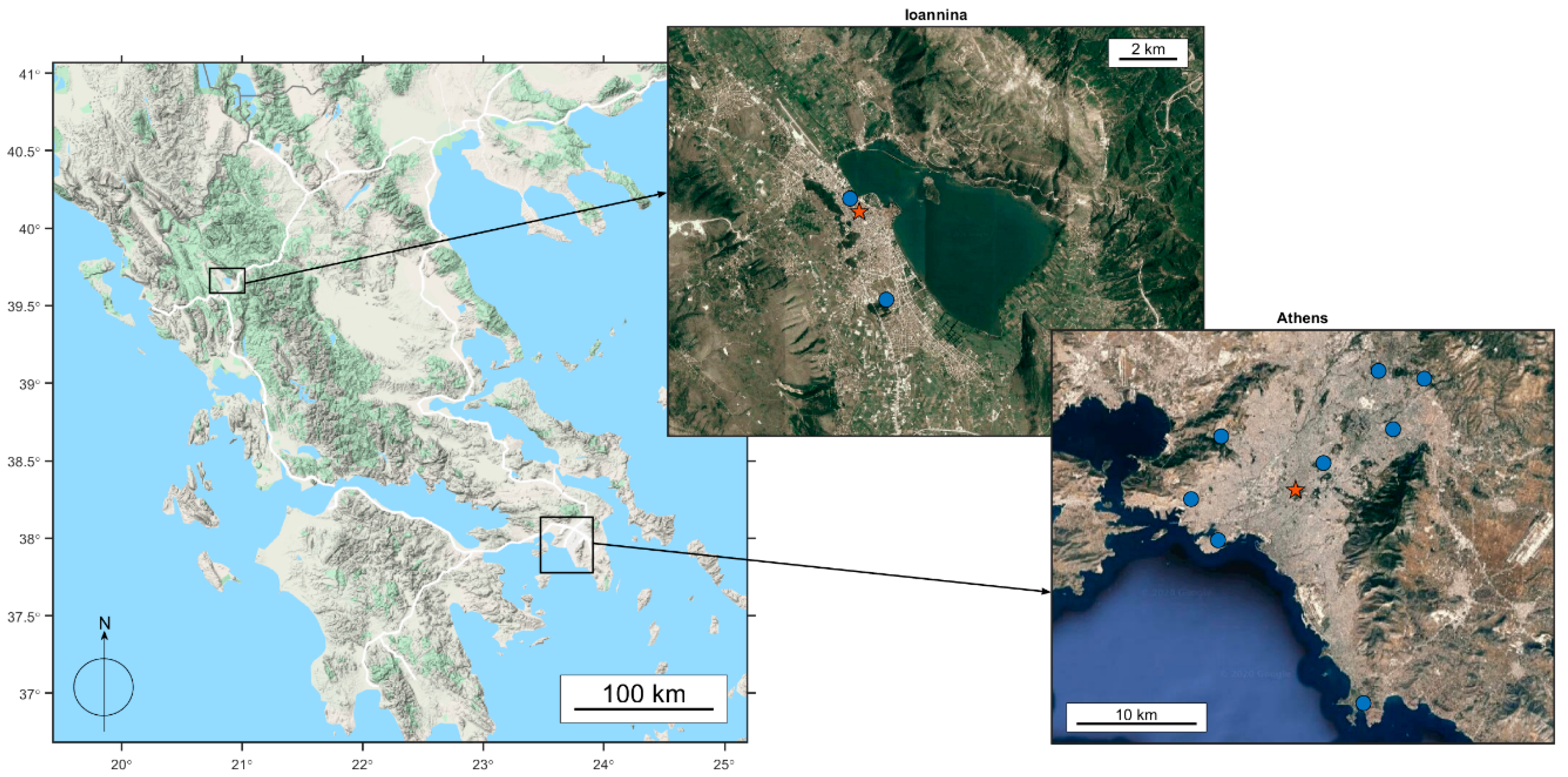
2.1. Sites and Measurement Periods

Field evaluation tests were held in two Greek cities, Athens and Ioannina, during 2019–2020. In Athens, the Greek capital and largest city with approximately four million inhabitants, measurements were performed at the Thissio urban background monitoring station (37.97326° N, 23.71836° E, 105 m ASL), operated by the National Observatory of Athens (NOA). The site is not directly affected by particle emissions, is located in an area of moderate population density, close to a large pedestrian zone and away from major roads. Therefore, it can be considered to be representative of background pollution in central Athens [38,39,40]. Initially, eight PA-II monitors were installed at Thissio for a nearly one-month period (8 March 2019–2 April 2019) during spring 2019. In a second phase, five PA-IIs were in operation at Thissio during summertime, from 3 July 2019 to 3 September 2019. In the third phase, during late winter and spring of 2020 (26 February 2020–18 May 2020), a single PA-II monitor (continuously operating since 7 July 2019 at the site, thus covering both calibration periods) was used. Table S1 summarizes information regarding each intercomparison campaign.

Ioannina is a medium-sized city in northwestern Greece with a population of approximately 100,000 inhabitants, located on a plateau in the foothills of the Pindus mountain range. Measurements in Ioannina were performed at the Vilara Air Quality Monitoring Station (39.67102° N, 20.84648° E, 484 m a.s.l.), operated by the Regional Authority of Epirus, in collaboration with the University of Ioannina. The station is located in the city center and is close to a road with moderate traffic. The intercomparison in Ioannina took place from 15 December 2019 until 31 May 2020, covering the spring period but also most of the winter period, when the city is heavily impacted by residential wood burning emissions, leading to persistent wintertime smog episodes [41].

Furthermore, several PA-II devices have been deployed at background locations within the larger urban zones of the two cities, with the objective to gradually form dense monitoring networks. In this study, we present results from nine such nodes in Athens and three in Ioannina. The network configuration, as well as the locations of the sites hosting reference instruments, can be seen in Figure 1, while details on the site characteristics are presented in Table S2 and Figure S1.

2.2. Instrumentation

2.2.1. The Purple Air PA-II Low-Cost PM Monitor

The PA-II monitor and its PA-II-SD version (PurpleAir LLC, Draper, UT, USA) incorporate a pair of PMS5003 (Plantower Ltd., Beijing, China) laser optical particle counter (OPC) sensors, along with a temperature, relative humidity, and barometric pressure sensor (BME 280, Bosch Sensortec GmbH, Reutlingen, Germany), both connected to a microcontroller equipped with a wireless network communication module. The device records and transmits data over Wi-Fi to a cloud-based platform, from where they can be downloaded at a 2 min. resolution. Pictures of the PA-II monitor and the PMS5003 sensor are provided in Figure S2. A side view with the twin-sensor design can be seen (Figure S2b), with air entering from four small holes in the bottom of the sensor and exiting from the fan at the same side. The sample flow is guided to the laser detector after two 90° turns. Drawn schematics on the internal sensor geometry and sample flow path can be found in Sayahi et al. [31] and Ardon-Dryer et al. [42].

The PMS5003 sensor provides digital outputs for 12 data fields. The first three correspond to the mass concentrations of PM₁, PM_2.5, and PM₁₀ fractions, without applying any correction, and they are labeled CF = 1. The next three, labeled CF = atm, correspond to adjusted mass concentrations derived after applying a proprietary algorithm developed by Plantower Ltd. The next six data fields contain the cumulative particle size distribution in six size ranges (>0.3 μm, >0.5 μm, >1 μm, >2.5 μm, >5 μm, and >10 μm). In addition to these parameters, from each of the two PM5003 sensors, the PA-II also reports data for temperature, relative humidity, and barometric pressure.

2.2.2. Reference Instrumentation

At Thissio, reference PM_2.5 concentration measurements were conducted using a reference-grade beta attenuation monitor (PX-375, Horiba Ltd., Kyoto, Japan), providing data that were averaged on a 3 h basis. The instrument was sampling through a PM₁₀ size-selective inlet upstream of a PM_2.5 sharp cut cyclone (VSCC 2.251, BGI Inc., Butler, NJ, USA) and was equipped with a sample heating system to avoid measurement bias due to variations in atmospheric moisture. In addition, a research-grade 31-channel optical particle counter (Model 11-D, Grimm Aerosol Technik, Ainring, Germany) was in operation at Thissio, sampling through a TSP sampling head, providing particle size distributions in the 0.2 μm to 35 μm range and mass concentrations for PM₁, PM_2.5, and PM₁₀, at a 1 min. resolution. Measurement data for meteorological parameters (ambient temperature—T, relative humidity—RH) were obtained from the adjacent NOA meteorological station, on an hourly basis.

In Ioannina a 32-channel optical particle counter (APDA-372, Horiba Ltd., Kyoto, Japan) was used as reference. The instrument is reference-equivalent for PM_2.5 and PM₁₀ measurement according to the EN 14907 and EN 12341 standards, respectively. It was sampling through a TSP sampling head with a vertical sampling line that was equipped with a particle drying system, providing mass concentrations of PM₁, PM_2.5 and PM₁₀ fractions on hourly intervals. Hourly average values of meteorological parameters (T, RH) were obtained using a, collocated, automated weather station.

2.2.3. Ancillary Measurements

Chemical composition of submicron aerosol at Thissio was monitored using an Aerosol Chemical Speciation Monitor (ACSM, Aerodyne Inc., Billerica, MA, USA) providing concentrations of the non-refractory (NR-PM₁) aerosol components (namely organic aerosol—OA, sulfate, nitrate, ammonium, and chloride) at a 30 min. resolution, complemented by Black Carbon (BC) measurements performed by a 7-λ aethalometer (AE-33, Magee Scientific, Berkeley, CA, USA) operating at a 1 min. resolution. Details on the operation and quality assurance regarding the ACSM can be found in Stavroulas et al. [43]. BC was also measured in Ioannina using again an AE-33 aethalometer at a 1 min. resolution. Furthermore, the aethalometer model [44,45] was used to calculate the fossil fuel (BC_ff) and biomass burning (BC_bb) fractions of black carbon, at both sites.

In order to support the identification of dust transport events, 120 h backward trajectories arriving at the two reference sites were calculated for selected periods, every 6 h at a height of 1000 m, using the HYSPLIT trajectory model [46], while PSCF (Potential Source Contribution Function) calculations were performed with the ZeFir toolkit developed for the Igor Pro software package [47].

2.3. Data Treatment

For the comparative evaluation and calibration of PA-II monitors, raw data from the two PMS5003 sensors in each monitor were averaged on 1 h time intervals. For the Athens datasets, in addition to 1 h average values for all of the examined parameters, 3 h averages were also calculated for comparisons with PM_2.5 reference concentrations from the beta-attenuation monitor. The agreement between the two individual sensors of each PA-II device was checked for hourly-averaged values and obvious outliers were excluded [20], however their frequency was negligible (< 0.05%).

Data capture (recovery) from the PA-II devices was very high (exceeding 99% for hourly average values at all sites, during all study periods), considerably exceeding the 90% threshold (that we indicatively mention as the minimum data capture rate required in reporting of continuous measurement data according to the EU air quality directive). Therefore, no imputation for missing values was performed. Data capture rates exceeding 99% have also been reported for the PA-II monitor by other studies [21], attesting to the device’s durability and consistent operation in field conditions.

The squared Pearson correlation coefficient (R²) is used throughout the manuscript as a correlation metric. PA-II PM_{2.5(CF = 1)} measurement biases in comparison to reference PM_2.5 are assessed through the mean bias error (MBE), the mean absolute error (MAE), and the normalized Root Mean Squared Error (nRMSE). These metrics are also used for analyzing the performance of the proposed calibration models. Bias errors correspond to the difference of the PA-II concentration minus the reference concentration. All related equations can be found in Section S1 of the supplement.

3. Results and Discussion

3.1. Field Evaluation and Device Calibration

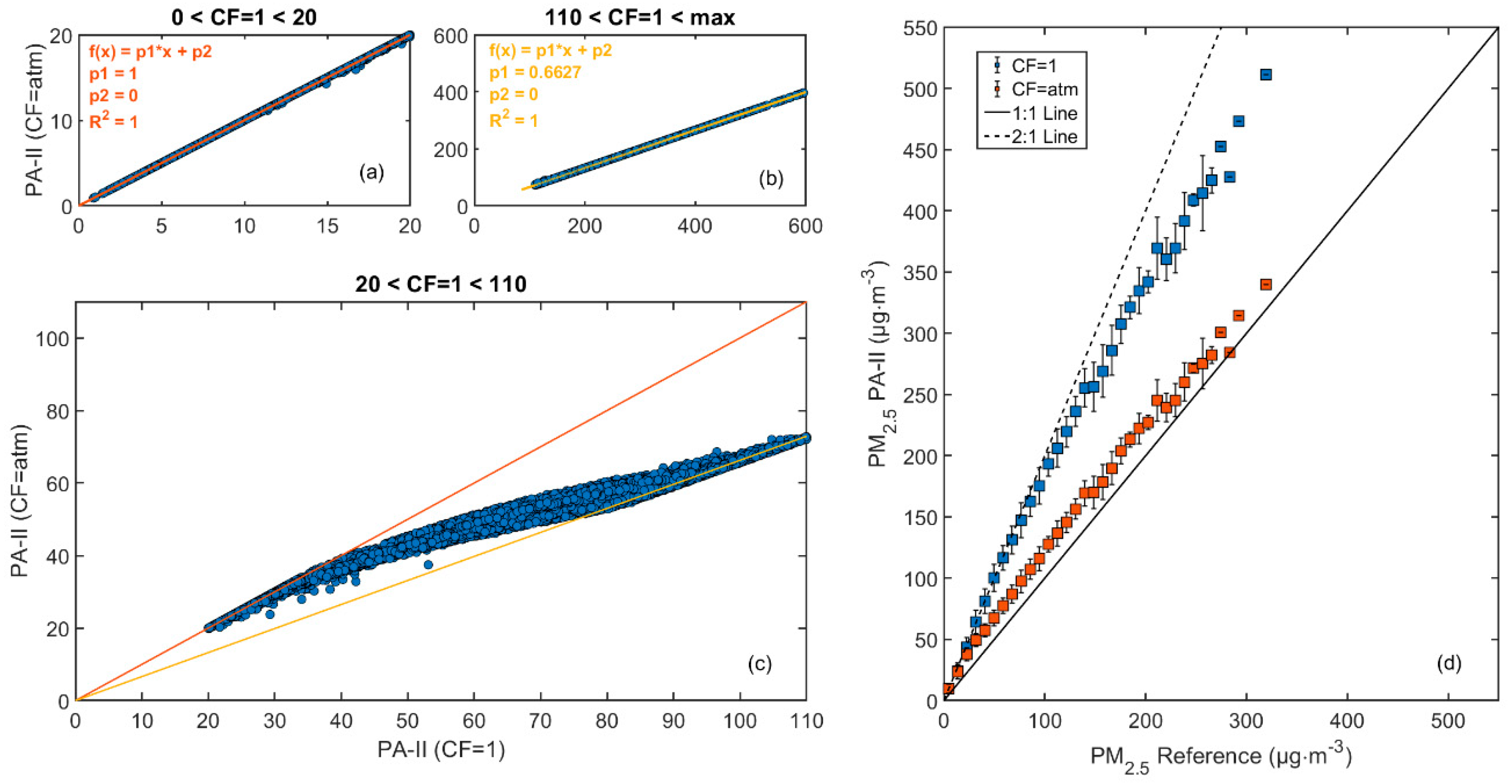
3.1.1. PM_2.5 Data Output of the PA-II Device

One of the main issues that need to be accounted for is which of the data fields (CF = 1, CF = atm), provided by the PMS5003 and, consequently, the PA-II monitor, should be considered when performing PM_2.5 field calibration, since the two outputs deviate notably in certain concentration ranges [25]. Examining the CF = 1 versus CF = atm scatterplots, a linear 1:1 relationship is observed for low concentrations. Then, a non-linear adjustment appears to be applied in mid-range CF = 1 values to derive CF = atm. Finally, another linear correction is applied for higher concentrations, with a coefficient that is smaller than one. Based on repeated observations on all datasets, the different PM_{2.5(CF = 1)} ranges (in μg m⁻³) where the three different corrections are applied to obtain PM_{2.5(CF = atm)}, are approximately the following:

• Low Range: PM_{2.5(CF = 1)} < 20, where PM_{2.5(CF = atm)} = PM_{2.5(CF = 1)}.
• Mid-Range: 20 < PM_{2.5(CF = 1)} < 110, where an unknown correction is applied by the sensor manufacturer.
• High Range: PM_{2.5(CF = 1)} > 110 where PM_{2.5(CF = atm)} ≈ 0.66 PM_{2.5(CF = 1)}.

To illustrate this, three scatterplots corresponding to the above concentration ranges, along with the linear regression equations for the first and third range are depicted in Figure 2a–c. The winter-time measurements in Ioannina were utilized for the visualization, as the dataset is characterized by a wide concentration range (hourly concentrations from as low as a few μg m⁻³ up to several hundreds of μg m⁻³). Splitting the reference dataset into 35 equidistant concentration bins that cover the entire ambient concentration range, calculating each bin’s PM_{2.5(CF = 1)} and PM_{2.5(CF = atm)} average, and finally plotting those values against the reference PM_2.5 values, leads to the plot of Figure 2d. It can be seen that for both data fields, while, at low concentrations binned averages follow a 2:1 line, they gradually deviate from it with increasing ambient concentrations.

A similar pattern has been reported for the PA-II monitor when comparing its outputs to a reference (TEOM) instrument [48], while non-linear fits with a similar curvature, as in Figure 2d, have been documented to better describe the sensor to reference relationship [31]. In Figure 2d, the pattern seems to be more pronounced for the CF = atm output, which, while falling on the 2:1 line for low concentrations, it tends towards the 1:1 line for higher ambient PM_2.5 levels. While this non-linear behavior of CF = atm should be addressed by any proposed calibration scheme, the use of the CF = 1 field may provide a more straightforward approach, also allowing for a more direct assessment of the effects that are related to aerosol physical properties, since there seems to be a more direct linkage between PM_{2.5(CF = 1)} and measured particle number concentrations. Thus, the CF = 1 field was utilized in the subsequent analysis. It is noted that the proprietary algorithm used for the correction of CF = 1 to CF = atm [31], to the best of our knowledge, has not been yet documented in the literature, is not available in the sensor manual or any relevant documentation, while it is also not known to the manufacturer of the PA-II monitor either (personal communication with Purple Air LLC).

3.1.2. Repeatability of PM_2.5 and T-RH Measurements

Eight devices—which subsequently were deployed at the various sites—were installed at the Thissio site during the 1st intercomparison period of 2019 in order to assess the repeatability of the PA-II monitor in ambient conditions. The results from pairwise comparisons of the PM_{2.5(CF = 1)} output of the devices are presented in Figure S3 and Table S3. The inter-device repeatability was high, with slopes and R² values very close to unity (0.98 < slope < 1.02, 0.997 <R² <1). Similar results supporting the high precision of the Purple Air PA-II monitor have been also documented by Feenstra et al. [21], using a triplet of PA-II devices. These results support the utilization of the device in low-cost PA-II networks, since they indicate the comparability of different monitors after their field deployment, and can facilitate different approaches for batch calibration.

A similar evaluation was performed for the temperature and relative humidity measurements by the BME280 sensors included in the PA-II devices. Precision is important in this case, since several calibration approaches utilize T and RH as inputs in order to minimize PA-II biases. For temperature, slopes varied in the range 0.82–1.10 and R² between 0.989 and 1, while, for relative humidity, ranges were 0.90 < slope < 1.07 and 0.996 < R² < 1, respectively. Detailed results regarding the pairwise comparisons of T-RH sensors can be found in Tables S4 through S7. When compared to reference T and RH measurements, the devices exhibit excellent linearity (Figure S4) but tend to overestimate temperature and underestimate relative humidity, probably owing to the BME sensor’s proximity to the electronics board inside the sensors’ housing [49].

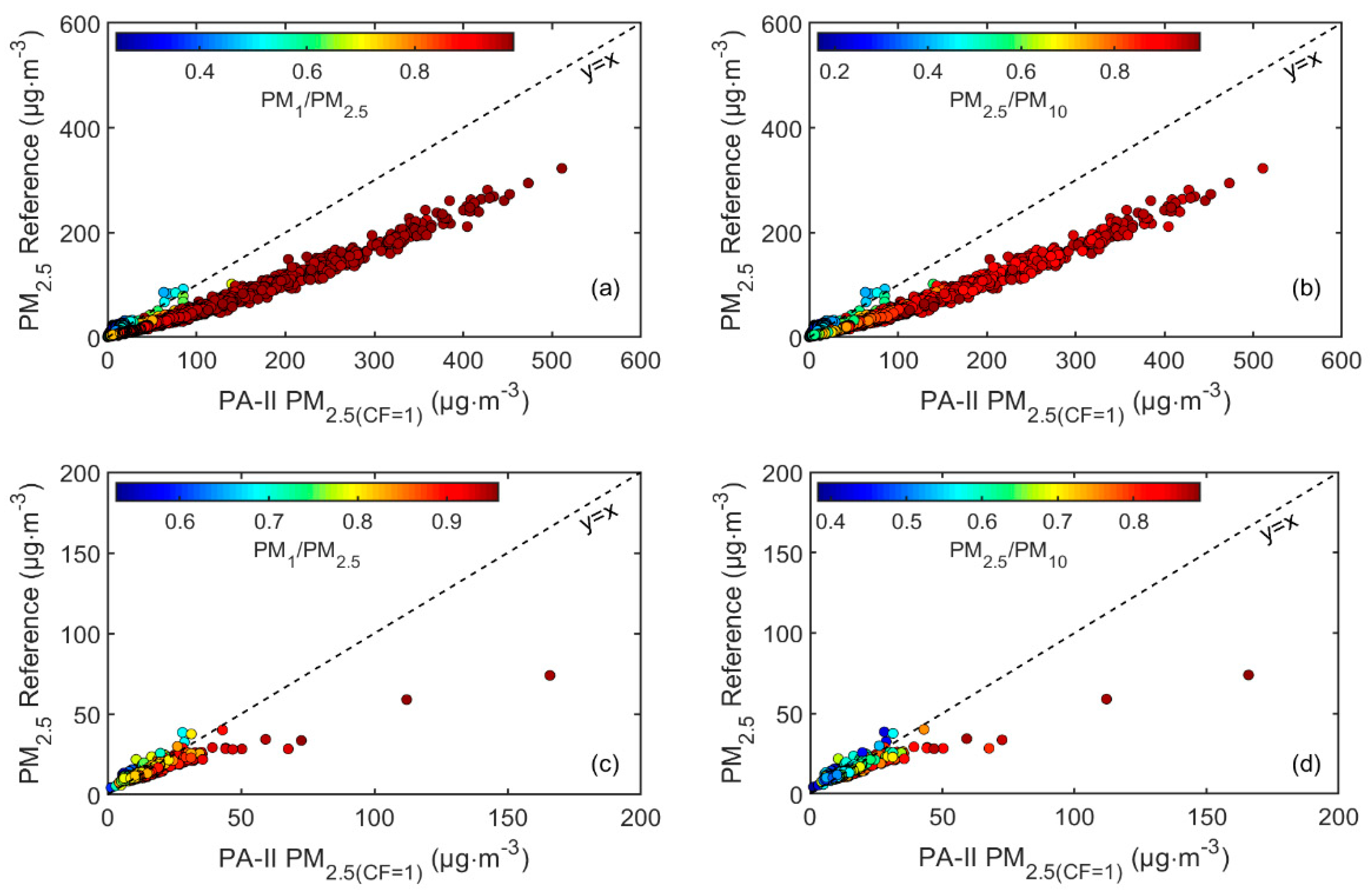
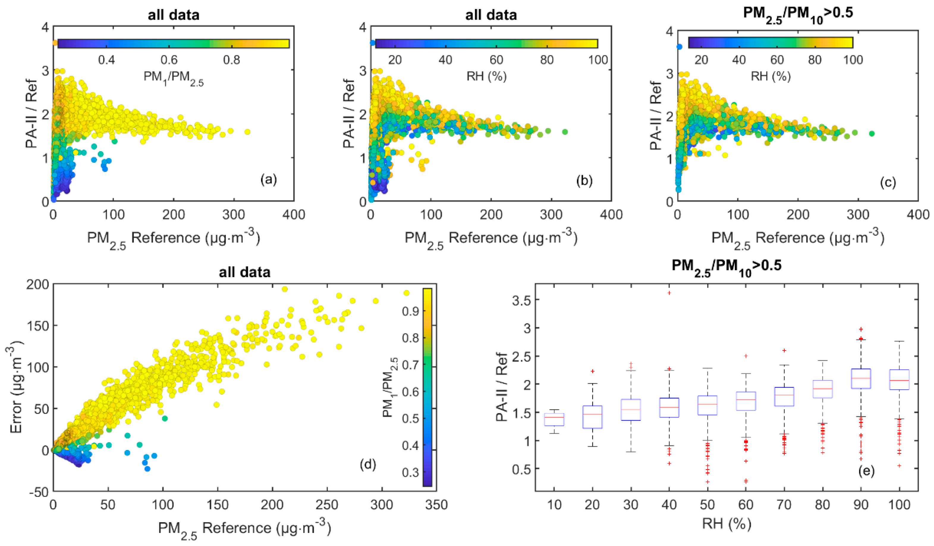
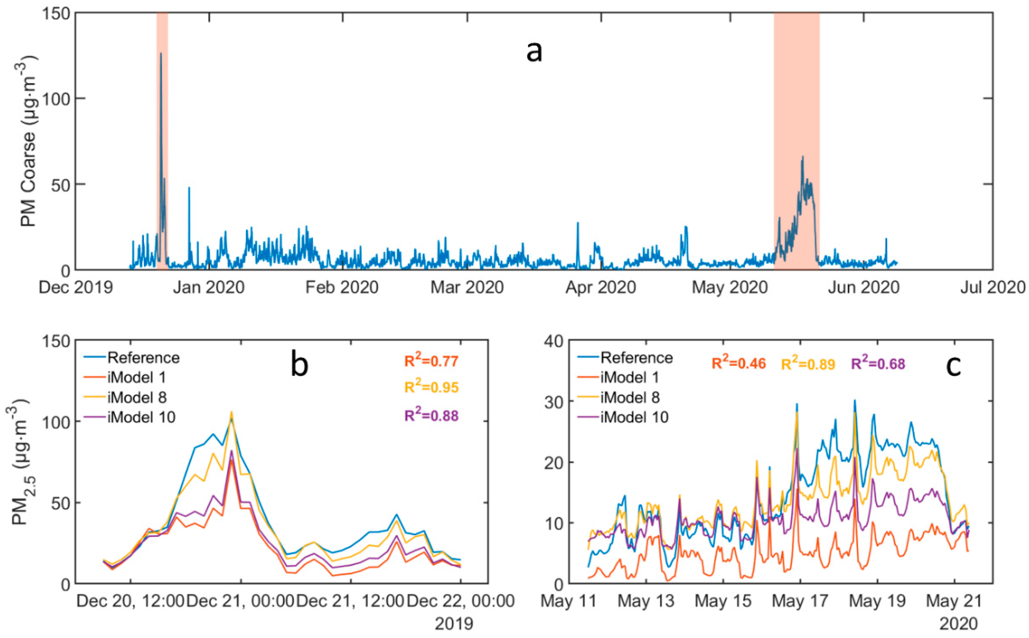
3.1.3. Coarse Particle and Relative Humidity Effects on Sensor Bias

During the intercomparison campaigns in Athens and Ioannina, the PA-II devices operated under a wide range of ambient conditions, regarding the meteorology, aerosol sources, and chemical composition. Furthermore, several dust episodes were observed, linked principally to air masses originating from northern Africa. Scatterplots of reference measurements conducted in Ioannina versus the PA-II PM_{2.5(CF = 1)} measurements can be seen in Figure 3a,b, providing an indication of coarse particle effects. Respectively, data from the 2nd Athens intercomparison campaign (the Grimm 11D OPC that provided the particle fraction ratios was not available during the 3rd intercomparison campaign) are depicted in Figure 3c,d.

The PMS5003 sensor has been documented to have poor size selectivity for coarse particles [30], while the design of the flow path—from inlet to optical cavity—forces the sample flow along two consecutive 90^o angles, favoring the deposition of larger particles before reaching the optical detector [31]. Therefore, the response is susceptible to error when aerosol is dominated by coarse particles, which in Southern European areas is typically observed during Saharan dust transport episodes [50].

In the present case, when color-coding data-points in the scatterplots according to their corresponding PM₁/PM_2.5 and PM_2.5/PM₁₀ ratios (calculated from measurements of the multi-channel OPC instruments), it is evident (Figure 3) that the data-points deviate from the general pattern for increasing coarse PM fractions (lower ratios). Points corresponding to lower ratios follow a steeper, almost 1:1 line, as compared to points corresponding to higher ratios, for which a clear overestimation by the PA-II is observed. Because these deviations become clearer when using PM₁/PM_2.5, this ratio will be henceforth used as a proxy in the related graphs.

On the other hand, important sensor biases can be expected in elevated ambient RH, since no conditioning of the sample takes place in the PMS5003 sensor. When evaluating the PA-II monitor, Magi et al. [51] reported linearly increasing MAE and RMSE errors with increasing RH, while a positive relationship between RH and MBE was documented by Feenstra et al. [21].

For the investigation of these effects, the absolute error of the PA-II PM_{2.5(CF = 1)} relative to the reference values in both datasets was first calculated. Given the fact that wintertime mean PM_2.5 concentrations in Ioannina were high (57.2 μg m⁻³), the analysis was initially focused on the springtime measurements (mean 13.4 μg m⁻³), in order to achieve comparability with the Athens dataset where the mean PM_2.5 concentration for the 2nd and 3rd campaigns combined was 15.2 μg m⁻³. Plotting the absolute error against the PM_2.5 reference concentrations, steeper slopes in the relationships with ambient concentrations were observed for higher RH values (Figure S5). This was more obvious in Ioannina, while, in Athens, this pattern was much less pronounced, probably due to the drier ambient conditions (RH: 49% in Athens versus 64% in Ioannina, on average, for the respective periods).

Data were divided in 20 equidistant bins according to RH, and the corresponding Mean Absolute Error (MAE) values was plotted, in order to examine the humidity effect. The results are shown in Figure S6, where an evident dependence of MAE on RH can be observed. The effect is more evident in the Ioannina dataset, with MAE rising from 8.5 μg m⁻³ to 35.7 μg m⁻³ when RH increases from 30% to 90%. This behavior could be linked to the frequent lake-effect fog events during wintertime in Ioannina [52], with the error being possibly related to water droplets that are introduced in the sample stream and counted in the PM_2.5 size range. A similar observation, with fog events inducing a positive bias in PM_2.5 measurements performed with the PMS1003 sensor—a previous version of PMS5003—has been also reported in Brisbane, Australia [53]. A positive but nevertheless more modest relationship can be observed in the Athens dataset, with MAE rising from 4.3 μg m⁻³ to 9.3 μg m⁻³ along the 30% to 90% RH increment.

It should be noted that higher concentration levels in Ioannina were mostly observed during the evening, coinciding with elevated RH levels. This means that part of the bias could be due to an additive effect of high concentration and RH, given the positive relationship between absolute error and ambient PM_2.5 levels (Figure S5). Other than that, the observations noted earlier, regarding the sensor behavior under elevated coarse mode concentrations (when the PA-II underestimates real PM_2.5 concentrations), implies that, in this case, the examination of the absolute error hinders the correct attribution of the actual measurement bias. Thus, it is necessary to isolate the influence of different effects and then examine their corresponding errors.

Because the RH and coarse particle effects tend to bias the performance in opposite directions, the bias error was examined as a metric of the sensor’s performance, for both Ioannina springtime and Athens datasets (Figure S7). The effect of coarse mode particles can be now observed clearly (Figure S7), with the majority of negative errors being calculated for low PM₁/PM_2.5 ratios, while a linear relationship with increasing concentration can be suggested for any PM₁/PM_2.5 ratio, starting with apparently negative slopes for low ratios and gradually moving towards positive slopes for higher ratios. A positive relationship with RH, even at mid-range concentrations is again suggested (Figure S6), while negative errors seem to be linked to lower RH, possibly related to drier and dust-laden southern air masses affecting continental Greece [54]. A boxplot of ΜBEs in 10% RH bins is also presented (Figure S7), where the RH dependence is obvious.

It is necessary to exclude that this increase was introduced by the positive error-concentration relationship to examine whether the increased bias linked to RH can be actually attributed to rising RH values. In this scope, the ratio of PA-II PM_{2.5(CF = 1)} to PM_2.5 reference concentrations (PA-II/Ref) was calculated and its association with the observed reference concentration was explored (Figure 4). In Figure 4a,b, data-points are color-coded by the PM₁/PM_2.5 ratio and RH respectively, and it is indicated that lower PM₁/PM_2.5 ratios correspond to low PA-II/Ref ratios (ranging from zero to roughly 1.5). We used the PM_2.5/PM₁₀ ratio (according to the analysis in Figure S8) in order to remove the points affected by the elevated coarse mode concentrations and consequently focus on the RH effect, given that, as an external parameter, it should be more readily available by regulatory monitoring stations, where, in most cases, PM₁ will not be routinely monitored. The colored scatterplot in Figure 4c, were coarse-related data-points (PM_2.5/PM₁₀ ratios less than 0.5) have been removed, clearly illustrates the RH effect on the sensor data deviation from reference dried measurements, while the resulting boxplot of Figure 4e points towards a linear pattern with the lower bin median PA-II/Ref at 1.41 and the higher at 2.10. A line was fitted to the calculated medians of each bin versus RH yielding an excellent correlation (R² = 0.96).

Through the error analysis, it is suggested that, in order to correct the PA-II PM_2.5 values, a multivariable approach should be followed, incorporating both humidity and coarse particle effects. The PA-II devices include a RH sensor, characterized by high repeatability (Section 3.1.2), which can be calibrated ahead of field deployment (Figure S4). However, the representative PM ratios required for corrections related to the presence of coarse mode particles should be externally provided. Such a solution could lie in the integration of PM_2.5, PM₁₀ data from a central or the nearest available regulatory air quality station (AQS), and it should be necessary when coarse-particle episodes are frequent and effective over wide urban areas. Similar calibration approaches have been already documented [20,55], albeit directly using reference PM_2.5 measurements coming from nearby regulatory AQS. Nevertheless, because lower PM ratios are not only related to regional phenomena, such as Saharan dust events in Southern Europe, this approach could face limitations regarding locally re-suspended dust. Therefore, its use in traffic sites, for example, where traffic induced resuspension can be substantial [56], may result in unsolicited errors.

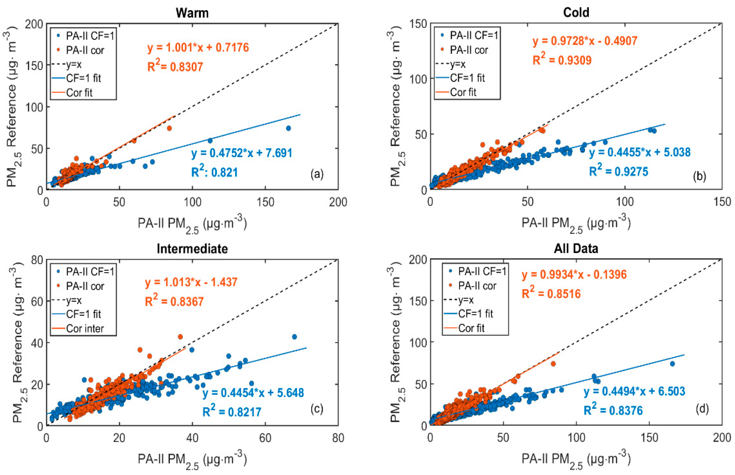
3.1.4. Models for Correction of PA-II PM_2.5 Measurements

• Models for Ioannina:

The Ioannina dataset was randomly divided in two subsets, selecting 60% as the base dataset (n = 2556 hourly observations) and the remaining 40% as the evaluation dataset (n = 1706) (Figure S9). The base dataset was used to fit different regression models. Reference PM_2.5 concentration was used as the dependent variable and PA-II PM_2.5 (CF = 1) concentration, ratios related to the presence of coarse particles (PM₁/PM_2.5 or PM_2.5/PM₁₀) and RH, were used as predictors. In total, ten different models were fitted, using all or a combination of the aforementioned predictors, starting with simple linear and quadratic regression models involving only the sensor and reference PM_2.5 data (iModel 1, iModel 2), then incorporating the PM ratios (iModel 3 to iModel6), and finally RH (iModel 7 to iModel 10). Motivation for including the PA-II PM_{2.5 (CF = 1)} as a squared term comes from the convex patterns observed in Figure 3, as well as the PA-II versus reference relationships documented in other studies [21,26,31]. A detailed description of the developed models can be found in Table S7. Generally, the larger part of the variability in the models can be explained by the PA-II PM_2.5 concentration variable. Positive increments with added predictors were somewhat small in terms of adjusted R², however coefficients of all added predictors were statistically significant at the 0.05 level, for all the models.

The obtained equations were then applied in the evaluation dataset and the model-corrected PA-II PM_2.5cor concentrations were compared to the reference measurements, calculating R², MAE, and normalized RMSE (nRMSE) as performance metrics.

Table 1. Performance metrics for the ten models tested in Ioannina (reference PM_2.5 versus the modeled PA-II PM_2.5cor) as calculated for the evaluation dataset.

Ioannina	R2	Slope	Intercept	nRMSE	MAE (μg m−3)
iModel 1	0.975	1.005	0.044	0.200	3.7
iModel 2	0.984	1.008	−0.012	0.162	2.9
iModel 3	0.983	1.007	−0.062	0.165	3.3
iModel 4	0.989	1.010	−0.112	0.135	2.7
iModel 5	0.983	1.006	0.034	0.168	3.4
iModel 6	0.987	1.008	−0.008	0.145	2.9
iModel 7	0.985	1.001	−0.044	0.158	2.9
iModel 8	0.992	1.004	−0.184	0.119	2.1
iModel 9	0.984	1.002	−0.091	0.166	3.2
iModel 10	0.988	1.005	−0.229	0.142	2.6

summarizes the results of the evaluation. The fitting ability of the models increased by progressively adding as predictors the variables that have been shown to directly influence the sensor’s measurement. Specifically, the nRMSE decreased by approximately 17% when the PM ratios were incorporated (iModel 3 and iModel 5) and approximately 21% when the polynomial model included also RH (iModel 7 and iModel 9), in comparison to the simple linear model (iModel 1). An important decrease (19%) in nRMSE, was also found by the simple quadratic models (iModel2), with no other external predictors. The model with the best descriptive power was the one incorporating PM₁/PM_2.5, RH, and a PA-II PM_{2.5(CF = 1)} quadratic term (iModel 8), yielding a 40% improvement in nRMSE, relative to the simple linear model. It is noted here that the PM_{2.5(CF = 1)} MAE, calculated for the evaluation dataset (before application of a correction model), was 25.4 μg m⁻³, much higher than the MAE of models, for which the lowest value was for iModel 8 (MAE = 2.2 μg m⁻³, 41% lower as compared to the simple linear iModel 1). Including PM ratios in the PA-II PM_2.5 calibration scheme appeared to drastically improve the behavior of the post-processed sensor signal during dust events.

Trying to discern which model incorporating the two coarse-related ratios (iModel 8 or iModel 10) performs better during a dust event, we focused on a severe dust episode recorded during 20–22 December 2019 and a milder event during 11–21 May 2020 in Ioannina. During these periods, air masses mostly originated from the southern sectors, with PSCF analysis indicating dust transport from north Africa (Figure S11), in agreement with the low PM_2.5/PM₁₀ ratios calculated. In Figure 5, the time-series of coarse PM as measured by the reference instrument is depicted, with the shaded areas corresponding to the respective dust events.

The mean PM_10-2.5 concentration was 38.7 μg m⁻³ during the December and 27.3 μg m⁻³ during the May event, in contrast to the 6.7 μg m⁻³ average that was registered for the entire period. In the bottom panels of Figure 5 the behavior of the two examined models along with the linear model (iModel 1) is shown. iModel 8 seems to generally perform better (Tables S10 and S11), yielding average PM_2.5 values that were closer to the recorded for each period (34.0 μg m⁻³ for December and 13.6 μg m⁻³ for May, against 37.7 and 14.2 μg m⁻³ that were measured by the reference instrument, respectively).

• Models for Athens:

The same approach was followed for the investigation of the best corrections applicable to the Athens intercomparison campaigns, using the beta attenuation monitor measurements as reference. As opposed to Ioannina, in Athens the models were not found to benefit from the inclusion of PA-II PM_{2.5(CF = 1)} as a quadratic term, since maximum ambient concentrations were relatively low (below 80 μg m⁻³ throughout the entire period; Figure 3). Because the PM₁/PM_2.5 and PM_2.5/PM₁₀ ratios data availability was limited to the 2nd Athens intercomparison campaign, multiple linear regression models incorporating those ratios were tested only for this period. Additionally, in Athens, models using only PA-II PM_{2.5(CF = 1)} and RH as predictors were tested, with data spanning both the 2nd and 3rd campaigns, after excluding data-points evidently affected by dust events. As criteria for this exclusion, we used: (i) a threshold of 0.5 for the PM_2.5/PM₁₀ ratio for the 2nd campaign (considering the analysis presented in Figure S8) and (ii) inspection of backward air mass trajectories when the PM_2.5/PM₁₀ ratio was not available.

The corresponding datasets were again randomly divided in base and evaluation subsets (60% and 40% respectively), creating in total four subsets (Figure S10). Six different regression models were tested and they are summarized in Tables S12 (configuration) and S13 (performance). The results for the evaluation datasets are summarized in

Table 2. Performance metrics for the various models tested in Ioannina (reference PM_2.5 versus the modeled PA-II PM_2.5cor) as calculated for the evaluation dataset.

Athens	R2	Slope	Intercept	nRMSE	MAE (μg m−3)
aModel 1 *	0.822	1.004	−0.273	0.198	2.2
aModel 2	0.838	1.326	−5.147	0.133	1.8
aModel 3	0.824	1.307	−4.950	0.139	1.9
aModel 4	0.817	1.269	−4.208	0.142	1.8
aModel 5	0.802	1.242	−3.870	0.147	1.8
aModel 6*	0.844	1.015	−0.439	0.186	2.0

* Data for both intercomparison campaigns (2nd and 3rd) at Thissio are used for aModel 1 and aModel 6.

. Once more, the models incorporating the coarse-related PM ratios (aModel 2 through aModel 5), exhibited the lowest nRMSE (0.133–0.147) and MAE (1.8 μg m⁻³) values and they were better correlated with the reference PM_2.5 measurements. Overall, the implementation of multiple regression models, resulted in an improvement of performance metrics, with aModel 4—the model incorporating the PM₁/PM_2.5 ratio and RH—corresponding to the smallest nRMSE (0.142) and MAE (1.8 μg m⁻³) values.

It is evident that correcting the raw sensor signal drastically improved the PA-II performance metrics for both the Ioannina and Athens datasets, effectively reducing MAE from 25.4 μg m⁻³ to below 3.7 μg m⁻³ and from 3.1 μg m⁻³ to below 2.2 μg m⁻³, respectively. Similar improvements have been observed by the majority of studies applying statistical models for correction. For example, Magi et al. [51] reported a 45% improvement in MAE after implementing a multilinear regression correction scheme, incorporating RH and reference PM_2.5 measurements as predictors, while Malings et al. [49], using more complex corrections by calculating an RH-related hygroscopic growth factor, documented a reduced MAE by 40%. Pawar et al. [57] applied a particle density adjustment followed by growth factor and aspiration efficiency corrections, reporting a 10–15% improvement in RMSE. Tryner et al. [48] reported that their correction (taking RH into account in a simple regression approach) reduced the absolute value of the mean bias from 2.1 to 0.6 μg m⁻³. Significant improvements in PA-II signal corrections have also been shown by the application of non-linear supervised machine learning approaches, such as artificial neural networks [58,59].

3.1.5. Comparison to Reference Instrumentation in Different Seasons

The corrected (aModel 6) PA-II output was examined against reference measurements at Thissio, in three different seasons during the 2nd and 3rd intercomparison campaigns, in order to assess the potential influence of seasonal factors on the performance of the PA-II monitor (that could be for example related to the seasonally variable chemical composition of urban aerosols).

The model choice was mainly dictated by the fact that the base dataset used in model aModel 6 was more representative, spanning all seasons in Athens, with the model displaying an overall good performance. The results are presented in Figure 6. Temperature and relative humidity diurnal patterns and basic statistics during those three seasons are presented in Table S14 and Figure S12. For the warm season (3 July 2019–3 September 2019, Figure 6a), the averaged PA-II PM_2.5cor and PM_{2.5(CF = 1)} data from the five installed PA-II devices at Thissio were used as independent variables in the displayed linear regressions. For the other two seasons, the cold (26 February 2020–7 April 2020) and intermediate (8 April 2020–19 May 2020), data from one PA-II deployed at Thissio were used as the independent variable. The cold and intermediate seasons were categorized according to long-term climatology studies for Southern Greece [60]. It is noted that, for the warm season data-points affected by coarse particles, according to criterion (i) described previously, were excluded, while for the intermediate and cold seasons, where no concurrent PM₁ or PM₁₀ measurements were available at Thissio, the affected data were excluded according to criterion (ii).

The comparisons indicate a relatively uniform response of the PA-II monitor, regardless of the measurement season in Athens, which is characteristic of consistent behavior for monitoring short-term PM_2.5 concentrations in the absence of elevated coarse mode concentrations. Furthermore, it is indicative that no significant drift in the sensor’s response was observed in the span of almost one year. The slopes of the linear regression of PM_2.5 reference versus PM_{2.5(CF = 1)}, range between 0.44 and 0.48, while the correlations remain excellent with R² varying in the range of 0.86 to 0.93. It must be noted that a statistically significant intercept was observed for the Thissio dataset, probably owing to the different operation principle of the compared instruments, with PMS5003 being limited to the direct detection of particles only larger than 0.3 μm [30].

On the other hand, the performance of selected models is considered to be satisfactory and consistent, yielding, in all seasons, small intercepts, slopes very close to unity, and excellent correlations to reference measurements, despite changes in chemical composition and aerosol source intensity year-round. The chemical composition and sources of aerosols have been extensively studied in the area of Athens. The main characteristics in urban/suburban background areas (such as those where devices were installed in the local network) are dominated by secondary aerosol throughout the year [38,56,61]. Ammonium sulfate is more abundant during summer, while secondary organics (especially the less oxidized fraction) are enhanced in the cold period [43]. Moreover, levels of primary organics and black carbon are largely enhanced during winter, mainly due to residential wood-burning emissions, while they diminish in summer, also due to decreased traffic [38,41,43,62]. The contribution of larger mineral dust particles in PM_2.5 is generally limited in the long-term (typically less than 10%). At background sites, where road-dust resuspension is limited, mineral dust is expected to contribute to PM_2.5 mostly during regional dust transport events [56].

It is possible that the content in primary organics and black carbon, which are typically emitted in the ultrafine range, is an additional error-inducing factor in the PA-II output, since particles with nominal diameters lower than 0.3 μm are not directly counted by the sensor. Actually, the mass fraction gathered in this size-range can be substantial. For example, Pennanen et al. [63] in central Athens has found 26% of PM_2.5 mass to be concentrated in sizes below 0.2 μm. These size ranges are dominated by organic and elemental carbon particles, while upper ranges (0.3–0.5 μm, 0.5–1 μm) are characterized by the increased presence of nitrate and sulfate particles [63,64,65]. However, aerosol ions are susceptible to water uptake which alters the scattering characteristics of sampled particles. Moreover, differences on apparent densities and shape factors of particles are related to their chemical characterization [66] and they can indirectly bias the sensor’s estimation algorithm that assumes fixed values [67].

The associations between measurement error and concentrations of source-specific aerosol components was examined in order to assess the potential effects of the seasonal variability of sources and chemical composition on the monitor’s performance. Small differences in error indicators have been found when evaluating the PA-II device in laboratory conditions for specific polydispersed particle sources with largely variable density and size distribution characteristics [25,27]. However, for ambient aerosols, where particle density is less variable and submicron aerosol dominates the PM_2.5 fraction [68], there is not much evidence on the chemical composition effects.

In the present case, the absolute error of PA-II PM_2.5cor (corrected with aModel6) relative to reference measurements was correlated against components that function as tracers of specific sources and atmospheric processes. The two aethalometer BC components (BC_ff and BC_bb) were used as indicators of traffic-related and biomass burning emissions (residential wood burning during the cold period and regional forest and agricultural fires during the warm) [69,70]. The sulfate concentrations that were determined using the ACSM were used to represent regional transported and processed secondary aerosol [43]. Comparisons were performed for the 2nd and 3rd Athens intercomparison campaigns; therefore, covering all three examined seasons (cold, warm, intermediate). Figure S13 shows the season-specific fine aerosol chemical composition measured by on-line instruments and Figure S14 the results of the comparison.

The results provide a first indication that the PA-II corrected signal is not directly affected by changes in chemical composition and intensity of examined sources. Correlations with aerosol type indicators in all cases were very weak (R² < 0.15). Additionally, the performance of the monitor remained stable when shifting from the warm to the cold period, which are characterized by distinct fine aerosol speciation. However, more work is needed in order to find an optimal way of investigating and addressing chemical composition effects and, furthermore, to explore links between the chemical composition and aerosol hygroscopic properties affecting the sensor’s performance in ambient conditions [49].

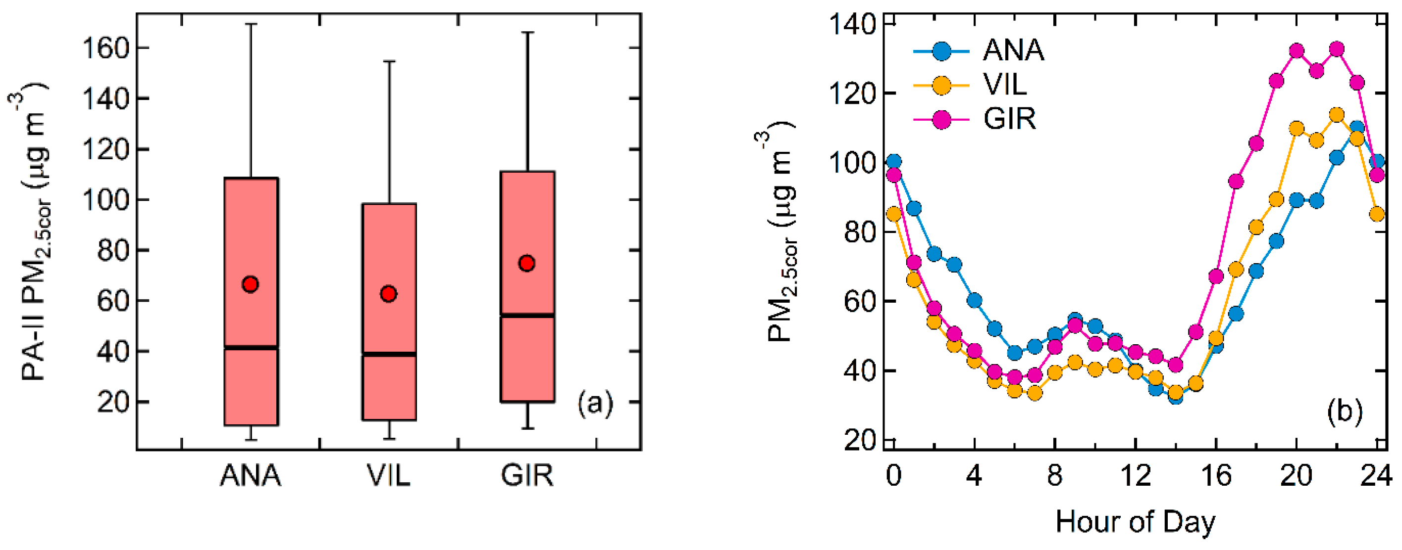
3.2. Monitoring PM_2.5 Using the PA-II in Greece

3.2.1. Athens

The performance of the PA-II network in Athens was evaluated during August 2019, when a large scale wildfire event took place in a forested mountainous area in Euboea, approximately 70 km to the N-NW of Athens, in an effort to assess the effectiveness of low-cost PM monitors, such as the PA-II, in providing alerts and real-time input to competent stakeholders, health experts and to the general public. The fire started in the late evening of August 12 and was active for almost three days. The transport of dense smoke plumes towards Athens was favored by the seasonally prevailing Etesian NW wind regime [71] and impacted on the Athens basin on August 13 and, to a lesser extent, during the following day. This can be also seen by satellite imagery (Figure S15) for the morning of August 13, when maximum hourly concentrations of 75–80 μg m⁻³ were recorded across the Athens basin at stations of the National Air Pollution Monitoring Network.

During this period, the PA-II monitoring network that was installed in the framework of the PANACEA project in Greece was operational, comprising of nine active devices, as presented in Figure 1. All PA-II data were corrected according to aModel 6 (using the PA-II RH corrected outputs). Figure 7 illustrates the August 13 time-series of the hourly corrected PM_2.5 concentrations, for all nine sensors. The first sites to be affected by the fire plume, were those on the western and northern parts of the Athens basin (HAI, PEF and CHA, see map in Figure S1), with concentration levels rising after 04:00 (local time), peaking at HAI at 07:00, while PEF and CHA, followed by the third northern site (MEL), reached maximum values at 08:00. The sites in the city center were affected after 06:00 with concentrations at THI (the Thissio central site) and GYZ reaching their maximum at 09:00, followed by a gradual decline till late afternoon. The two sites in the southern zone around the port of Piraeus (KER and PIR) were the last to be affected, mainly after 08:00, exhibiting maxima at 10:00–11:00 along with a new maximum at the nearby western HAI site. Performing a simple nearest neighbor interpolation [72] on a 0.01° grid (Figure S16), for every hourly averaged set of measurements, the evolution of the plume’s influence on the basin can be illustrated, with some generalization of the effect to areas that surround each site.

The degree of spatial homogeneity between the hourly PM_2.5 measurements in the nine urban/suburban background sites was also assessed during the entire month of August. The coefficient of divergence (CoD, Section S1) and squared correlation coefficient (R²) were calculated for each site-pair, after excluding the wildfire event, and the results are presented in

Table 3. Coefficient of divergence (CoD) values for each pair of monitoring sites in Athens during August 2019, excluding the days that the basin was impacted by the Euboea wildfire plume.

	THI	GYZ	PEF	PIR	MEL	CHA	VOU	KER
GYZ	0.07
PEF	0.08	0.06
PIR	0.11	0.12	0.13
MEL	0.09	0.08	0.05	0.14
CHA	0.08	0.07	0.05	0.14	0.06
VOU	0.13	0.12	0.12	0.19	0.12	0.11
KER	0.09	0.09	0.09	0.09	0.11	0.10	0.16
HAI	0.08	0.09	0.09	0.10	0.10	0.10	0.15	0.05

and Section S14. In general, values of CoD that are closer to zero are related to higher spatial homogeneity [73]. A high degree of spatial homogeneity for PM_2.5 can be seen across sites, as the CoD values were found below 0.2, which is considered as a threshold value ([74] and references therein). The mean CoD value was 0.10 (ranging between 0.05–0.16), very similar to the mean CoD value of 0.09 found by Lianou et al. [75] for PM_2.5 measurements at 35 residential sites in the greater area of Athens. Generally, inter-site distance appears to be inversely related with CoD, with lower values between sites in the same sectors of the basin, as, for example, can be observed by the very low values (0.05–0.06) between the three sites in the north sector (CHA, MEL, PEF).

The low CoD results are mainly due to the similar characterization of sites (urban background or suburban background), which are not directly affected by local emissions. They also extend past results for CoD values regarding PM₁₀ measured at numerous locations in the Athens basin, which, in the case of background site-pairs, ranged between 0.17–0.21 [76]. The exclusion of the coarse fraction is expected to lead to smaller CoD [77], especially in the present case, where dust-related PM_2.5 are not effectively measured. On the contrary, higher than 0.2 CoD values have been documented in Athens for fine and coarse particles in traffic vs. urban background site-pairs [56]. At background locations within the Athens basin, several source apportionment studies have identified secondary species as the main component of background fine aerosols [38,56,78]. Due to the regional scale of processing and transport of secondary aerosol, its levels are spatially uniform over the entire area [56], leading to a higher degree of uniformity for PM_2.5 particles as well. It should be also noted that the impact of traffic sources, that is already limited in background locations, is further decreased during the August vacation period in Athens [62].

Two sites that present different characteristics in Figure 7 are PIR and VOU, which were associated with CoD values almost consistently larger than 0.10. Concentrations at VOU, a suburban background site at a relatively large distance from the city center (18.5 km from Thissio), were lower than in the other sites (mean concentration of 13.1 μg m⁻³). Meanwhile, PM_2.5 concentrations in PIR (Piraeus), an area where the largest European passenger port is located—at the peak of its capacity during summer [79]—appear to be affected by the activity related to the port, with a primary maximum in early morning (07:00 LT) linked to the traffic rush hour and secondary maxima during the evening related to passenger ship departures and arrivals [80].

3.2.2. Ioannina

Studies in Ioannina have revealed the important effect of residential wood burning in elevated fine aerosol concentrations during wintertime [41,81]. Three PA-II devices were deployed (Figure 1, Figure S1), specifically at two urban background (VIL, GIR) and one suburban background (ANA) site, in order to monitor the spatial variability of PM_2.5 concentrations in the city. During the 13 December 2019–13 January 2020 period, pollution in Ioannina was dominated by residential wood burning, as inferred by concurrent aethalometer (AE-33, Magee Scientific) measurements at the city center. During this period an average BC concentration of 5.02 μg m⁻³ was measured, with hourly maxima up to 31 μg m⁻³ and a very high contribution of BC_bb (75% on average). In fact, during the night hours (18:00–6:00 local time), BC concentrations were almost completely attributed to biomass burning, with the BC_bb contribution rising to 88%.

In this context, PA-II PM_2.5cor concentrations, corrected according to iModel 8, were calculated for the three sites. The selection of the model is primarily dictated by the need to compensate for the intense regional dust event observed during December 20 to December 22 (Figure S11), but it is also based on the fact that all of the stations are relatively close to the regulatory AQS site (VIL), 3.1 and 0.5 km, respectively, for ANA and GIR (in contrast to an average inter-site distance of 9 km for Athens), thus allowing for uniform use of the AQS (VIL site) measured PM₁/PM_2.5 ratio. Very high PM_2.5cor levels (Figure 8a) were determined at all sites, with average concentrations for the monthly period ranging between 62.8–74.8 μg m⁻³. Higher concentrations were measured at the GIR site, located in a street-canyon of a densely populated neighborhood in the city center. However, the high-concentration event appeared to be effective over the larger urban zone of Ioannina, with comparable levels also recorded at the suburban background ANA site. Hourly maxima reached 350 μg m⁻³ at all sites, while the frequency of hourly measurements above 100 μg m⁻³ was 29%, 27%, and 24% at GIR, ANA, and VIL, respectively, with the vast majority of these observations recorded during nighttime.

Focusing on the diurnal variability during the examined one-month period (Figure 8b), it appears that, for all sites, maximum concentrations were recorded during nighttime, capturing the important role of wood combustion for residential heating, with GIR—representing a typical residential area—exhibiting the highest night-time peak. Secondary maxima were observed during the morning traffic rush hour at all sites, with the central VIL site being the least affected. The ANA site, although located in a suburban area, is close to the major international motorway connecting the city, which is burdened with heavy traffic [82], while GIR is located close to the main road traversing the Ioannina Lake shore and leading to the city airport. These differences in the monitoring sites characteristics were also reflected on the moderate spatial heterogeneity inferred by the pairwise CoD calculation. The GIR-ANA sites exhibited the highest differences with CoD = 0.33, while levels at the central VIL site were fairly uniform with the other two sites (CoD: 0.23–0.24), indicating its suitability as a representative background location for PM_2.5 measurements in the city (Tables S16 and S17).

4. Conclusions

In recent years, low-cost PM monitors, which are based on optical particle counting/sizing technology, are widely used to monitor PM levels, providing a cost-effective and practical solution. As their performance is strongly dependent on environmental factors, including humidity and abundance of coarse particles, which vary seasonally, but also spatially, extensive work is required to better understand their response and propose suitable calibration procedures. This task was addressed in the present study, by examining the performance of the Purple Air PA-II sensor, on both seasonal and spatial scales, and in two contrasting environments in Greece: Athens, the capital of Greece with more than four-million inhabitants and Ioannina, a medium-sized city in northwestern Greece, affected by residential wood burning emissions in winter, rendering it one of the most polluted cities of Greece, during that season. The main results of this study are summarized below:

• The CF = 1 data field provided by the PMS5003 sensor was considered more appropriate to calibrate the PA-II device, as it displayed better linear behavior against reference measurements and without the necessity to interpret the sensor’s black-box data processing.
• The PA-II temperature and relative humidity sensor proved to be robust, linear, and easy to calibrate, allowing for temperature and relative humidity data use in correction approaches.
• The presence of—mainly dust related—coarse particles, along with elevated ambient relative humidity conditions, have been identified as important sources of measurement bias and a limiting factor for a uniform correction, due to area and site specificities.
• Polynomial multiple regression models can improve the PA-II performance and minimize biases that are related to relative humidity levels and coarse-to-fine particle fractionation. However, such corrections should be applied locally and additional work is needed to check their applicability at a regional scale. In this sense and given that the gains in performance, although indicative of the effects, were not very pronounced, it has to be weighted whether they justify the additional required work and dataflow as compared to simple calibration using only reference PM measurements.
• The correlations found between the PA-II monitor and reference PM_2.5 were notably higher in the case of the reference optical monitor than for the beta-gauge monitor, mainly attributed to the similar operating principle. Intercomparison experiments for PA-II against different collocated reference instruments, and also comparisons with the same reference instrument at multiple locations, will substantially broaden the scope of research.

The PA-II performance appears to remain rather stable in the mid-to-long term, regardless of seasonal fluctuations in ambient conditions and aerosol chemical composition; however, more detailed work is required in order to assess the latter. Overall, the installation of dense PA-II networks, complementing regulatory AQS networks, can improve our knowledge on the spatial variability of PM concentrations and population exposure, in general and especially during local or regional pollution events affecting the urban landscape. The potential availability of concentration data from tens of measurement locations in a large city can prove rather useful for health studies in order to develop more representative spatial models for population exposure and minimize exposure misclassification errors due to within-area variability of concentrations. Moreover, as most low-cost networks operate frequently according to open-data principles, they can provide useful data to the research community and broaden the scope of air quality research.

Sensor-based monitoring and citizen networks are emerging solutions as it becomes clear that future urban air quality management should be integrated in a smart city framework. In this sense, a diffuse utilization of air quality sensor-based monitors, while it can provide a wealth of real-time data with high spatial resolution, can also lead to inaccurate estimations of the air quality status or misuse by third parties, if proper calibration is not applied. Direct comparison of uncorrected measurements with air quality standards should be avoided and this should be emphasized as much as possible. Therefore, more research and strategic planning is necessary regarding the optimal incorporation of low-cost devices in operational monitoring networks, with focus on their reliable calibration and the possibility for automation in calibration procedures. Furthermore, more work is needed in order to link caveats in the performance of the PA-II monitor to physical and chemical properties of sampled aerosol. Future research should include testing of the device in controlled laboratory conditions by chamber experiments, also evaluating solutions for the mitigation of the identified humidity and particle size distribution effects.

References

- Brook, R.D.; Rajagopalan, S.; Pope, C.A., III; Brook, J.R.; Bhatnagar, A.; Diez-Roux, A.V.; Holguin, F.; Hong, Y.; Luepker, R.V.; Mittleman, M.A.; et al. Particulate matter air pollution and cardiovascular disease: An update to the scientific statement from the American Heart Association. Circulation 2010, 121, 2331–2378. [Google Scholar] [CrossRef]
- Olstrup, H.; Johansson, C.; Forsberg, B.; Tornevi, A.; Ekebom, A.; Meister, K. A multi-pollutant air quality health index (AQHI) based on short-term respiratory effects in Stockholm, Sweden. Int. J. Environ. Res. Pub. Health 2019, 16, 105. [Google Scholar] [CrossRef]
- Liu, C.; Chen, R.; Sera, F.; Vicedo-Cabrera, A.M.; Guo, Y.; Tong, S.; Coelho, M.S.; Saldiva, P.H.; Lavigne, E.; Matus, P.; et al. Ambient particulate air pollution and daily mortality in 652 cities. N. Eng. J. Med. 2019, 381, 705–715. [Google Scholar] [CrossRef] [PubMed]
- Lelieveld, J.; Pozzer, A.; Pöschl, U.; Fnais, M.; Haines, A.; Münzel, T. Loss of life expectancy from air pollution compared to other risk factors: A worldwide perspective. Cardiovasc. Res. 2020. [Google Scholar] [CrossRef] [PubMed]
- European Environment Agency. Air Quality in Europe—2019; Report No 10/2019; Publications Office of the European Union: Luxembourg, 2019; pp. 66–70. [Google Scholar]
- Lipsett, M.J.; Ostro, B.D.; Reynolds, P.; Goldberg, D.; Hertz, A.; Jerrett, M.; Smith, D.F.; Garcia, C.; Chang, E.T.; Bernstein, L. Long-term exposure to air pollution and cardiorespiratory disease in the California teachers study cohort. Am. J. Respir. Crit. Care Med. 2011, 184, 828–835. [Google Scholar] [CrossRef] [PubMed]
- Shi, L.; Zanobetti, A.; Kloog, I.; Coull, B.A.; Koutrakis, P.; Melly, S.J.; Schwartz, J.D. Low-concentration PM2.5 and mortality: Estimating acute and chronic effects in a population-based study. Environ. Health Perspect. 2016, 124, 46–52. [Google Scholar] [CrossRef] [PubMed]
- Cesaroni, G.; Forastiere, F.; Stafoggia, M.; Andersen, Z.J.; Badaloni, C.; Beelen, R.; Caracciolo, B.; de Faire, U.; Erbel, R.; Eriksen, K.T.; et al. Long term exposure to ambient air pollution and incidence of acute coronary events: Prospective cohort study and meta-analysis in 11 European cohorts from the ESCAPE Project. Br. Med. J. 2014, 348, f7412. [Google Scholar] [CrossRef]
- Di, Q.; Wang, Y.; Zanobetti, A.; Wang, Y.; Koutrakis, P.; Choirat, C.; Dominici, F.; Schwartz, J.D. Air pollution and mortality in the Medicare population. N. Eng. J. Med. 2017, 376, 2513–2522. [Google Scholar] [CrossRef] [PubMed]
- World Health Organization. Air Quality Guidelines: Global Update 2005: Particulate Matter, Ozone, Nitrogen Dioxide, and Sulfur Dioxide; WHO Regional Office for Europe: Copenhagen, Denmark, 2006; pp. 217–305. [Google Scholar]
- World Health Organization. Ambient Air Pollution: A global Assessment of Exposure and Burden of Disease; WHO Document Production Services: Geneva, Switzerland, 2016. [Google Scholar]
- Zhang, Z.; Whitsel, E.A.; Quibrera, P.M.; Smith, R.L.; Liao, D.; Anderson, G.L.; Prineas, R.J. Ambient Fine Particulate Matter Exposure and Myocardial Ischemia in the Environmental Epidemiology of Arrhythmogenesis in the Women’s Health Initiative (EEAWHI) Study. Environ. Health Perspect. 2009, 117, 751–756. [Google Scholar] [CrossRef]
- Atkinson, R.W.; Kang, S.; Anderson, H.R.; Mills, I.C.; Walton, H.A. Epidemiological time series studies of PM2.5 and daily mortality and hospital admissions: A systematic review and meta-analysis. Thorax 2014, 69, 660–665. [Google Scholar] [CrossRef]
- Weichenthal, S.; Kulka, R.; Lavigne, E.; Van Rijswijk, D.; Brauer, M.; Villeneuve, P.J.; Stieb, D.; Joseph, L.; Burnett, R.T. Biomass burning as a source of ambient fine particulate air pollution and acute myocardial infarction. Epidemiology 2017, 28, 329. [Google Scholar] [CrossRef] [PubMed]
- Delfino, R.J.; Brummel, S.; Wu, J.; Stern, H.; Ostro, B.; Lipsett, M.; Winer, A.; Street, D.H.; Zhang, L.; Tjoa, T.; et al. The relationship of respiratory and cardiovascular hospital admissions to the southern California wildfires of 2003. Occup. Environ. Med. 2009, 66, 189–197. [Google Scholar] [CrossRef] [PubMed]
- Kumar, P.; Morawska, L.; Martani, C.; Biskos, G.; Neophytou, M.; Di Sabatino, S.; Bell, M.; Norford, L.; Britter, R. The rise of low-cost sensing for managing air pollution in cities. Environ. Int. 2015, 75, 199–205. [Google Scholar] [CrossRef] [PubMed]
- Jiao, W.; Hagler, G.; Williams, R.; Sharpe, R.; Brown, R.; Garver, D.; Judge, R.; Caudill, M.; Rickard, J.; Davis, M.; et al. Community Air Sensor Network (CAIRSENSE) project: Evaluation of low-cost sensor performance in a suburban environment in the southeastern United States. Atmos. Meas. Tech. 2016, 9, 5281–5292. [Google Scholar] [CrossRef]
- Gao, M.; Cao, J.; Seto, E. A distributed network of low-cost continuous reading sensors to measure spatiotemporal variations of PM2.5 in Xi’an, China. Environ. Pollut. 2015, 199, 56–65. [Google Scholar] [CrossRef]
- Park, H.S.; Kim, R.E.; Park, Y.; Hwang, K.C.; Lee, S.H.; Kim, J.J.; Choi, J.Y.; Lee, D.G.; Chang, L.S.; Choi, W. The potential of commercial sensors for spatially dense short-term air quality monitoring based on multiple short-term evaluations of 30 sensor nodes in urban areas in Korea. Aerosol Air Qual. Res. 2020, 20, 369–380. [Google Scholar] [CrossRef]
- Bi, J.; Wildani, A.; Chang, H.H.; Liu, Y. Incorporating low-cost sensor measurements into high-resolution PM2.5 modeling at a large spatial scale. Environ. Sci. Technol. 2020, 54, 2152–2162. [Google Scholar] [CrossRef]
- Feenstra, B.; Papapostolou, V.; Hasheminassab, S.; Zhang, H.; Der Boghossian, B.; Cocker, D.; Polidori, A. Performance evaluation of twelve low-cost PM2.5 sensors at an ambient air monitoring site. Atmos. Environ. 2019, 216, 116946. [Google Scholar] [CrossRef]
- Borrego, C.; Ginja, J.; Coutinho, M.; Ribeiro, C.; Karatzas, K.; Sioumis, T.; Katsifarakis, N.; Konstantinidis, K.; De Vito, S.; Esposito, E.; et al. Assessment of air quality microsensors versus reference methods: The EuNetAir Joint Exercise—Part II. Atmos. Environ. 2018, 193, 127–142. [Google Scholar] [CrossRef]
- Tagle, M.; Rojas, F.; Reyes, F.; Vásquez, Y.; Hallgren, F.; Lindén, J.; Kolev, D.; Watne, Å.K.; Oyola, P. Field performance of a low-cost sensor in the monitoring of particulate matter in Santiago, Chile. Environ. Monitor. Assess. 2020, 192, 171. [Google Scholar] [CrossRef]
- Kelleher, S.; Quinn, C.; Miller-Lionberg, D.; Volckens, J. A low-cost particulate matter (PM2.5) monitor for wildland fire smoke. Atmos. Meas. Tech. 2018, 11, 1087–1097. [Google Scholar] [CrossRef]
- Kelly, K.E.; Whitaker, J.; Petty, A.; Widmer, C.; Dybwad, A.; Sleeth, D.; Martin, R.; Butterfield, A. Ambient and laboratory evaluation of a low-cost particulate matter sensor. Environ. Pollut. 2017, 221, 491–500. [Google Scholar] [CrossRef] [PubMed]
- Zheng, T.; Bergin, M.H.; Johnson, K.K.; Tripathi, S.N.; Shirodkar, S.; Landis, M.S.; Sutaria, R.; Carlson, D.E. Field evaluation of low-cost particulate matter sensors in high- and low-concentration environments. Atmos. Meas. Tech. 2018, 11, 4823–4846. [Google Scholar] [CrossRef]
- Levy Zamora, M.; Xiong, F.; Gentner, D.; Kerkez, B.; Kohrman-Glaser, J.; Koehler, K. Field and laboratory evaluations of the low-cost Plantower Particulate Matter sensor. Environ. Sci. Technol. 2019, 53, 838–849. [Google Scholar] [CrossRef]
- He, M.; Kuerbanjiang, N.; Dhaniyala, S. Performance characteristics of the low-cost Plantower PMS optical sensor. Aerosol Sci. Technol. 2020, 54, 232–241. [Google Scholar] [CrossRef]
- Wang, Y.; Li, J.; Jing, H.; Zhang, Q.; Jiang, J.; Biswas, P. Laboratory evaluation and calibration of three low-cost particle sensors for particulate matter measurement. Aerosol Sci. Technol. 2015, 49, 1063–1077. [Google Scholar] [CrossRef]
- Kuula, J.; Mäkelä, T.; Aurela, M.; Teinilä, K.; Varjonen, S.; González, Ó.; Timonen, H. Laboratory evaluation of particle-size selectivity of optical low-cost particulate matter sensors. Atmos. Meas. Tech. 2020, 13, 2413–2423. [Google Scholar] [CrossRef]
- Sayahi, T.; Kaufman, D.; Becnel, T.; Kaur, K.; Butterfield, A.E.; Collingwood, S.; Zhang, Y.; Gaillardon, P.E.; Kelly, K.E. Development of a calibration chamber to evaluate the performance of low-cost particulate matter sensors. Environ. Pollut. 2019, 255, 113–131. [Google Scholar] [CrossRef]
- Kim, S.; Park, S.; Lee, J. Evaluation of performance of inexpensive laser based PM2.5 sensor monitors for typical indoor and outdoor hotspots of South Korea. App. Sci. 2019, 9, 1947. [Google Scholar] [CrossRef]
- Mehadi, A.; Moosmüller, H.; Campbell, D.E.; Ham, W.; Schweizer, D.; Tarnay, L.; Hunter, J. Laboratory and field evaluation of real-time and near real-time PM2.5 smoke monitors. J. Air Waste Manag. Assoc. 2020, 70, 158–179. [Google Scholar] [CrossRef]
- Crilley, L.R.; Shaw, M.; Pound, R.; Kramer, L.J.; Price, R.; Young, S.; Lewis, A.C.; Pope, F.D. Evaluation of a low-cost optical particle counter (Alphasense OPC-N2) for ambient air monitoring. Atmos. Meas. Tech. 2018, 11, 709–720. [Google Scholar] [CrossRef]
- Sahu, R.; Dixit, K.K.; Mishra, S.; Kumar, P.; Shukla, A.K.; Sutaria, R.; Tiwari, S.; Tripathi, S.N. Validation of low-cost sensors in measuring real-time PM10 concentrations at two sites in Delhi national capital region. Sensors 2020, 20, 1347. [Google Scholar] [CrossRef] [PubMed]
- Karagulian, F.; Barbiere, M.; Kotsev, A.; Spinelle, L.; Gerboles, M.; Lagler, F.; Redon, N.; Crunaire, S.; Borowiak, A. Review of the performance of low-cost sensors for air quality monitoring. Atmosphere 2019, 10, 506. [Google Scholar] [CrossRef]
- Field Evaluation: Purple Air PM-II PM Sensor; Air-Quality Sensor Performance Evaluation Center (AQ-SPEC); SCAQMD: Diamond Bar, CA, USA, 2017. Available online: http://www.aqmd.gov/docs/default-source/aq-spec/field-evaluations/purple-air-pa-ii---field-evaluation.pdf (accessed on 21 July 2017).
- Theodosi, C.; Tsagkaraki, M.; Zarmpas, P.; Grivas, G.; Liakakou, E.; Paraskevopoulou, D.; Lianou, M.; Gerasopoulos, E.; Mihalopoulos, N. Multi-year chemical composition of the fine-aerosol fraction in Athens, Greece, with emphasis on the contribution of residential heating in wintertime. Atmos. Chem. Phys. 2018, 18, 14371–14391. [Google Scholar] [CrossRef]
- Grivas, G.; Stavroulas, I.; Liakakou, E.; Kaskaoutis, D.G.; Bougiatioti, A.; Paraskevopoulou, D.; Gerasopoulos, E.; Mihalopoulos, N. Measuring the spatial variability of black carbon in Athens during wintertime. Air Qual. Atmos. Health 2019, 12, 1405–1417. [Google Scholar] [CrossRef]
- Athanasopoulou, E.; Speyer, O.; Brunner, D.; Vogel, H.; Vogel, B.; Mihalopoulos, N.; Gerasopoulos, E. Changes in domestic heating fuel use in Greece: Effects on atmospheric chemistry and radiation. Atmos. Chem. Phys. 2017, 17, 10597–10618. [Google Scholar] [CrossRef]
- Kaskaoutis, D.G.; Grivas, G.; Theodosi, C.; Tsagkaraki, M.; Paraskevopoulou, D.; Stavroulas, I.; Liakakou, E.; Gkikas, A.; Hatzianastassiou, N.; Wu, C.; et al. Carbonaceous aerosols in contrasting atmospheric environments in Greek cities: Evaluation of the EC-tracer methods for secondary organic carbon estimation. Atmosphere 2020, 11, 161. [Google Scholar] [CrossRef]
- Ardon-Dryer, K.; Dryer, Y.; Williams, J.N.; Moghimi, N. Measurements of PM2.5 with PurpleAir under atmospheric conditions. Atmos. Meas. Tech. Discuss. 2019, 1–33. [Google Scholar] [CrossRef]
- Stavroulas, I.; Bougiatioti, A.; Grivas, G.; Paraskevopoulou, D.; Tsagkaraki, M.; Zarmpas, P.; Liakakou, E.; Gerasopoulos, E.; Mihalopoulos, N. Sources and processes that control the submicron organic aerosol composition in an urban Mediterranean environment (Athens): A high temporal-resolution chemical composition measurement study. Atmos. Chem. Phys. 2019, 19, 901–919. [Google Scholar] [CrossRef]
- Sandradewi, J.; Prévôt, A.S.; Szidat, S.; Perron, N.; Alfarra, M.R.; Lanz, V.A.; Weingartner, E.; Baltensperger, U. Using aerosol light absorption measurements for the quantitative determination of wood burning and traffic emission contributions to particulate matter. Environ. Sci. Technol. 2008, 42, 3316–3323. [Google Scholar] [CrossRef]
- Drinovec, L.; Močnik, G.; Zotter, P.; Prévôt, A.S.H.; Ruckstuhl, C.; Coz, E.; Rupakheti, M.; Sciare, J.; Müller, T.; Wiedensohler, A.; et al. The "dual-spot" Aethalometer: An improved measurement of aerosol black carbon with real-time loading compensation. Atmos. Meas. Tech. 2015, 8, 1965–1979. [Google Scholar] [CrossRef]
- Stein, A.F.; Draxler, R.R.; Rolph, G.D.; Stunder, B.J.; Cohen, M.D.; Ngan, F. NOAA’s HYSPLIT atmospheric transport and dispersion modeling system. Bull. Am. Meteorol. Soc. 2015, 96, 2059–2077. [Google Scholar] [CrossRef]
- Petit, J.-E.; Favez, O.; Albinet, A.; Canonaco, F. A user-friendly tool for comprehensive evaluation of the geographical origins of atmospheric pollution: Wind and trajectory analyses. Environ. Model. Soft. 2017, 88, 183–187. [Google Scholar] [CrossRef]
- Tryner, J.; L’Orange, C.; Mehaffy, J.; Miller-Lionberg, D.; Hofstetter, J.C.; Wilson, A.; Volckens, J. Laboratory evaluation of low-cost PurpleAir PM monitors and in-field correction using co-located portable filter samplers. Atmos. Environ. 2020, 220, 117067. [Google Scholar] [CrossRef]
- Malings, C.; Tanzer, R.; Hauryliuk, A.; Saha, P.K.; Robinson, A.L.; Presto, A.A.; Subramanian, R. Fine particle mass monitoring with low-cost sensors: Corrections and long-term performance evaluation. Aerosol Sci. Technol. 2020, 54, 160–174. [Google Scholar] [CrossRef]
- Gerasopoulos, E.; Kouvarakis, G.; Babasakalis, P.; Vrekoussis, M.; Putaud, J.P.; Mihalopoulos, N. Origin and variability of particulate matter (PM10) mass concentrations over the Eastern Mediterranean. Atmos. Environ. 2006, 40, 4679–4690. [Google Scholar] [CrossRef]
- Magi, B.I.; Cupini, C.; Francis, J.; Green, M.; Hauser, C. Evaluation of PM2.5 measured in an urban setting using a low-cost optical particle counter and a Federal Equivalent Method Beta Attenuation Monitor. Aerosol Sci. Technol. 2020, 54, 147–159. [Google Scholar] [CrossRef]
- Houssos, E.E.; Lolis, C.J.; Gkikas, A.; Hatzianastassiou, N.; Bartzokas, A. On the atmospheric circulation characteristics associated with fog in Ioannina, north-western Greece. Int. J. Climatol. 2012, 32, 1847–1862. [Google Scholar] [CrossRef]
- Jayaratne, R.; Liu, X.; Thai, P.; Dunbabin, M.; Morawska, L. The influence of humidity on the performance of a low-cost air particle mass sensor and the effect of atmospheric fog. Atmos. Meas. Tech. 2018, 11, 4883–4890. [Google Scholar] [CrossRef]
- Dimitriou, K.; Kassomenos, P. Estimation of North African dust contribution on PM10 episodes at four continental Greek cities. Ecol. Indic. 2019, 106, 105530. [Google Scholar] [CrossRef]
- Becnel, T.; Sayahi, T.; Kelly, K.; Gaillardon, P.E. A recursive approach to partially blind calibration of a pollution sensor network. In Proceedings of the IEEE International Conference on Embedded Software and Systems (ICESS), Las Vegas, NV, USA, 2–3 June 2019; pp. 1–8. [Google Scholar] [CrossRef]
- Grivas, G.; Cheristanidis, S.; Chaloulakou, A.; Koutrakis, P.; Mihalopoulos, N. Elemental composition and source apportionment of fine and coarse particles at traffic and urban background locations in Athens, Greece. Aerosol Air Qual. Res. 2018, 18, 1642–1659. [Google Scholar] [CrossRef]
- Pawar, H.; Sinha, B. Humidity, density, and inlet aspiration efficiency correction improve accuracy of a low-cost sensor during field calibration at a suburban site in the North-Western Indo-Gangetic plain (NW-IGP). Aerosol Sci. Technol. 2020, 54, 685–703. [Google Scholar] [CrossRef]
- Sachit, M.; Kumar, P. Evaluation of low-cost sensors for quantitative personal exposure monitoring. Sustain. Cities Soc. 2020, 57, 102076. [Google Scholar] [CrossRef]
- Si, M.; Xiong, Y.; Du, S.; Du, K. Evaluation and calibration of a low-cost particle sensor in ambient conditions using machine-learning methods. Atmos. Meas. Tech. 2020, 13, 1693–1707. [Google Scholar] [CrossRef]
- Argiriou, A.A.; Kassomenos, P.A.; Lykoudis, S.P. On the methods for the delimitation of seasons. Water Air Soil Pollut. Focus 2004, 4, 65–74. [Google Scholar] [CrossRef]
- Paraskevopoulou, D.; Liakakou, E.; Gerasopoulos, E.; Theodosi, C.; Mihalopoulos, N. Long-term characterization of organic and elemental carbon in the PM2.5 fraction: The case of Athens, Greece. Atmos. Chem. Phys. 2014, 14, 13313–13325. [Google Scholar] [CrossRef]
- Liakakou, E.; Stavroulas, I.; Kaskaoutis, D.G.; Grivas, G.; Paraskevopoulou, D.; Dumka, U.C.; Tsagkaraki, M.; Bougiatioti, A.; Oikonomou, K.; Sciare, J.; et al. Long-term variability, source apportionment and spectral properties of black carbon at an urban background site in Athens, Greece. Atmos. Environ. 2020, 222, 117137. [Google Scholar] [CrossRef]
- Pennanen, A.S.; Sillanpää, M.; Hillamo, R.; Quass, U.; John, A.C.; Branis, M.; Hůnová, I.; Meliefste, K.; Janssen, N.A.H.; Koskentalo, T.; et al. Performance of a high-volume cascade impactor in six European urban environments: Mass measurement and chemical characterization of size-segregated particulate samples. Sci. Total Environ. 2007, 374, 297–310. [Google Scholar] [CrossRef]
- Cass, G.R.; Hughes, L.A.; Bhave, P.; Kleeman, M.J.; Allen, J.O.; Salmon, L.G. The chemical composition of atmospheric ultrafine particles. Philos. Trans. A Math. Phys. Eng. Sci. 2000, 358, 2581–2592. [Google Scholar] [CrossRef]
- Chow, J.C.; Watson, J.G.; Lowenthal, D.H.; Magliano, K.L. Size-resolved aerosol chemical concentrations at rural and urban sites in Central California, USA. Atmos. Res. 2008, 90, 243–252. [Google Scholar] [CrossRef]
- Pitz, M.; Schmid, O.; Heinrich, J.; Birmili, W.; Maguhn, J.; Zimmermann, R.; Wichmann, H.-E.; Peters, A.; Cyrys, J. Seasonal and diurnal variation of PM2.5 apparent particle density in urban air in Augsburg, Germany. Environ. Sci. Technol. 2008, 42, 5087–5093. [Google Scholar] [CrossRef] [PubMed]
- Bulot, F.M.J.; Russell, H.S.; Rezaei, M.; Loxham, M.; Cox, S.J. Laboratory comparison of low-cost particulate matter sensors to measure transient events of pollution. Sensors 2020, 20, 2219. [Google Scholar] [CrossRef] [PubMed]
- Theodosi, C.; Grivas, G.; Zarmpas, P.; Chaloulakou, A.; Mihalopoulos, N. Mass and chemical composition of size-segregated aerosols (PM1, PM2.5, PM10) over Athens, Greece: Local versus regional sources. Atmos. Chem. Phys. 2011, 11, 11895–11911. [Google Scholar] [CrossRef]
- Sciare, J.; Oikonomou, K.; Favez, O.; Liakakou, E.; Markaki, Z.; Cachier, H.; Mihalopoulos, N. Long-term measurements of carbonaceous aerosols in the Eastern Mediterranean: Evidence of long-range transport of biomass burning. Atmos. Chem. Phys. 2008, 8, 5551–5563. [Google Scholar] [CrossRef]
- Liakakou, E.; Kaskaoutis, D.G.; Grivas, G.; Stavroulas, I.; Tsagkaraki, M.; Paraskevopoulou, D.; Bougiatioti, A.; Dumka, U.C.; Gerasopoulos, E.; Mihalopoulos, N. Long-term brown carbon spectral characteristics in a Mediterranean city (Athens). Sci. Total Environ. 2020, 708, 135019. [Google Scholar] [CrossRef]
- Kalkavouras, P.; Bougiatioti, A.; Grivas, G.; Stavroulas, I.; Kalivitis, N.; Liakakou, E.; Gerasopoulos, E.; Pilinis, C.; Mihalopoulos, N. On the regional aspects of new particle formation in the Eastern Mediterranean: A comparative study between a background and an urban site based on long term observations. Atmos. Res. 2020, 104911. [Google Scholar] [CrossRef]
- Wong, D.W.; Yuan, L.; Perlin, S.A. Comparison of spatial interpolation methods for the estimation of air quality data. J. Expo. Sci. Environ. Epidemiol. 2004, 14, 404–415. [Google Scholar] [CrossRef]
- Pinto, J.P.; Lefohn, A.S.; Shadwick, D.S. Spatial variability of PM2.5 in urban areas in the United States. J. Air Waste Manag. Assoc. 2004, 54, 440–449. [Google Scholar] [CrossRef]
- Wilson, J.G.; Kingham, S.; Pearce, J.; Sturman, A.P. A review of intraurban variations in particulate air pollution: Implications for epidemiological research. Atmos. Environ. 2005, 39, 6444–6462. [Google Scholar] [CrossRef]
- Lianou, M.; Chalbot, M.C.; Kotronarou, A.; Kavouras, I.G.; Karakatsani, A.; Katsouyanni, K.; Puustinnen, A.; Hameri, K.; Vallius, M.; Pekkanen, J.; et al. Dependence of home outdoor particulate mass and number concentrations on residential and traffic features in urban areas. J. Air Waste Manag. Assoc. 2007, 57, 1507–1517. [Google Scholar] [CrossRef]
- Grivas, G.; Chaloulakou, A.; Kassomenos, P. An overview of the PM10 pollution problem, in the Metropolitan Area of Athens, Greece. Assessment of controlling factors and potential impact of long-range transport. Sci. Total Environ. 2008, 389, 165–177. [Google Scholar] [CrossRef] [PubMed]
- Massoud, R.; Shihadeh, A.L.; Roumié, M.; Youness, M.; Gerard, J.; Saliba, N.; Zaarour, R.; Abboud, M.; Farah, W.; Saliba, N.A. Intraurban variability of PM10 and PM2.5 in an Eastern Mediterranean city. Atmos. Res. 2011, 101, 893–901. [Google Scholar] [CrossRef]
- Paraskevopoulou, D.; Liakakou, E.; Gerasopoulos, E.; Mihalopoulos, N. Sources of atmospheric aerosol from long-term measurements (5 years) of chemical composition in Athens, Greece. Sci. Total Environ. 2015, 527–528, 165–178. [Google Scholar] [CrossRef] [PubMed]
- Tzannatos, E. Ship emissions and their externalities for the port of Piraeus–Greece. Atmos. Environ. 2010, 44, 400–407. [Google Scholar] [CrossRef]
- Kassomenos, P.A.; Vardoulakis, S.; Chaloulakou, A.; Paschalidou, A.K.; Grivas, G.; Borge, R.; Lumbreras, J. Study of PM10 and PM2.5 levels in three European cities: Analysis of intra and inter urban variations. Atmos. Environ. 2014, 87, 153–163. [Google Scholar] [CrossRef]
- Sindosi, O.A.; Markozannes, G.; Rizos, E.; Ntzani, E. Effects of economic crisis on air quality in Ioannina, Greece. J. Environ. Sci. Health A 2019, 54, 768–781. [Google Scholar] [CrossRef] [PubMed]
- Tsogas, G.Z.; Giokas, D.L.; Vlessidis, A.G.; Aloupi, M.; Angelidis, M.O. Survey of the distribution and time-dependent increase of platinum-group element accumulation along urban roads in Ioannina (NW Greece). Water Air Soil Pollut. 2009, 201, 265–281. [Google Scholar] [CrossRef]