The Summer Surface Energy Budget of the Ice-Free Area of Northern James Ross Island and Its Impact on the Ground Thermal Regime

Abstract

Despite the key role of the surface energy budget in the global climate system, such investigations are rare in Antarctica. In this study, the surface energy budget measurements from the largest ice-free area on northern James Ross Island, in Antarctica, were obtained. The components of net radiation were measured by a net radiometer, while sensible heat flux was measured by a sonic anemometer and ground heat flux by heat flux plates. The surface energy budget was compared with the rest of the Antarctic Peninsula Region and selected places in the Arctic and the impact of surface energy budget components on the ground thermal regime was examined. Mean net radiation on James Ross Island during January–March 2018 reached 102.5 W m⁻². The main surface energy budget component was the latent heat flux, while the sensible heat flux values were only 0.4 W m⁻² lower. Mean ground heat flux was only 0.4 Wm^-2, however, it was negative in 47% of January–March 2018, while it was positive in the rest of the time. The ground thermal regime was affected by surface energy budget components to a depth of 50 cm. The strongest relationship was found between ground heat flux and ground surface temperature. Further analysis confirmed that active layer refroze after a sequence of three days with negative ground heat flux even in summer months. Daily mean net radiation and ground heat flux were significantly reduced when cloud amount increased, while the influence of snow cover on ground surface temperature was negligible.

1. Introduction

Polar regions with their vast ice-sheets are important climatic factors influencing the climate of the whole planet. The white surface of glaciers in Antarctica and in the Arctic has an albedo of up to 90% [1], thereby reflecting incoming shortwave radiation and reducing the amount of energy available to the Earth. In the Antarctic, the net amount of incoming solar radiation further affects the grade of turbulent fluxes, atmospheric circulation on a large scale and, as a consequence, the energy budget of the whole planet.

More than 99% of Antarctica is covered by ice [2], but the ice-free area is further predicted to enlarge [3,4,5], especially in the Antarctic Peninsula (AP) region. Despite the fact that warming in the AP region has decelerated or even been absent since the 2000s, large decadal [6] and spatial variability in air temperature [7] was found to be a typical feature in this area. Therefore, it does not necessarily indicate a return to a colder climate from a long-term perspective [8].

Most studies have analysed the surface energy budget over sea-ice, snow and ice-covered areas (e.g., [9,10,11,12]). Ice-free areas, such as in the AP region, on the other hand, have received less attention. Choi et al. [13] reported that the mean monthly net radiation on an ice-free area on King George Island (KGI) was more than two-times larger than the values reported for glaciers in the AP region [9,10,14]. Unlike over ice-covered areas, ice-free ground in high latitudes can also be a heat source for the atmosphere [15]. Furthermore, coastal sites are affected by sea proximity, for instance by increased moisture availability for sublimation when the sea is free of ice [16]. However, studies on the surface energy budget in ice-free areas have failed to agree on how the energy is portioned into turbulent and ground heat fluxes [13,15,17], which may be connected to the loss of the low-frequency fluctuation part of fluxes [18]. Thus, further research might help explain the discrepancies.

Moreover, the surface energy budget in cold regions is, to a large extent, affected by snow cover (e.g., [19]). Net radiation in polar regions is limited due to the existence of snow and ice-covered areas, which have up to six times larger albedo compared with bare surfaces [1]. Furthermore, the heat exchange between the ground and the atmosphere is lowered because of snow insulation [20]. Apart from that, reduced ground heat loss weakens the soil temperature decrease [21,22]. Knowledge on how the surface energy budget influences the Antarctic ground thermal regime and how its interaction with snow cover modifies the ground temperature remains limited [17]. Nevertheless, it would be beneficial for improving the knowledge on energy fluxes, weather forecast validation and improvements in the temporal and spatial resolution of numerical models [13].

Surface energy budget studies from ice-free areas in Antarctica only relate to South Shetland Archipelago [13,17]. To the best of our current knowledge, no surface energy budget research has been carried out on the north-eastern side of the AP. Yet, the largest ice-free area, the Ulu Peninsula on James Ross Island (JRI), lies in this region. The sparse vegetation coastal areas of northern JRI resemble semi-desert conditions, such as in Svalbard or Greenland, in terms of vegetation cover, soil and water content [23,24].

The lack of data increases the level of uncertainty about regional climate projections which are also crucial to the assessment of the response of biotic and abiotic components of Antarctic terrestrial ecosystems. The climatic conditions on the eastern side of the AP are known to differ from the western side (e.g., [25]). Correspondingly, the link between the active layer thickness and the surface energy budget in the eastern AP region remains unknown. The main objectives of this study are:

• To quantify the summer surface energy budget over the ice-free area on the Ulu Peninsula;
• To identify the connection between components of the surface energy budget and verify if the energy fluxes differ between the western and eastern side of the AP; and
• To determine the effect of snow cover and cloudiness on the surface energy budget and ground thermal regime.

2. Material and Methods

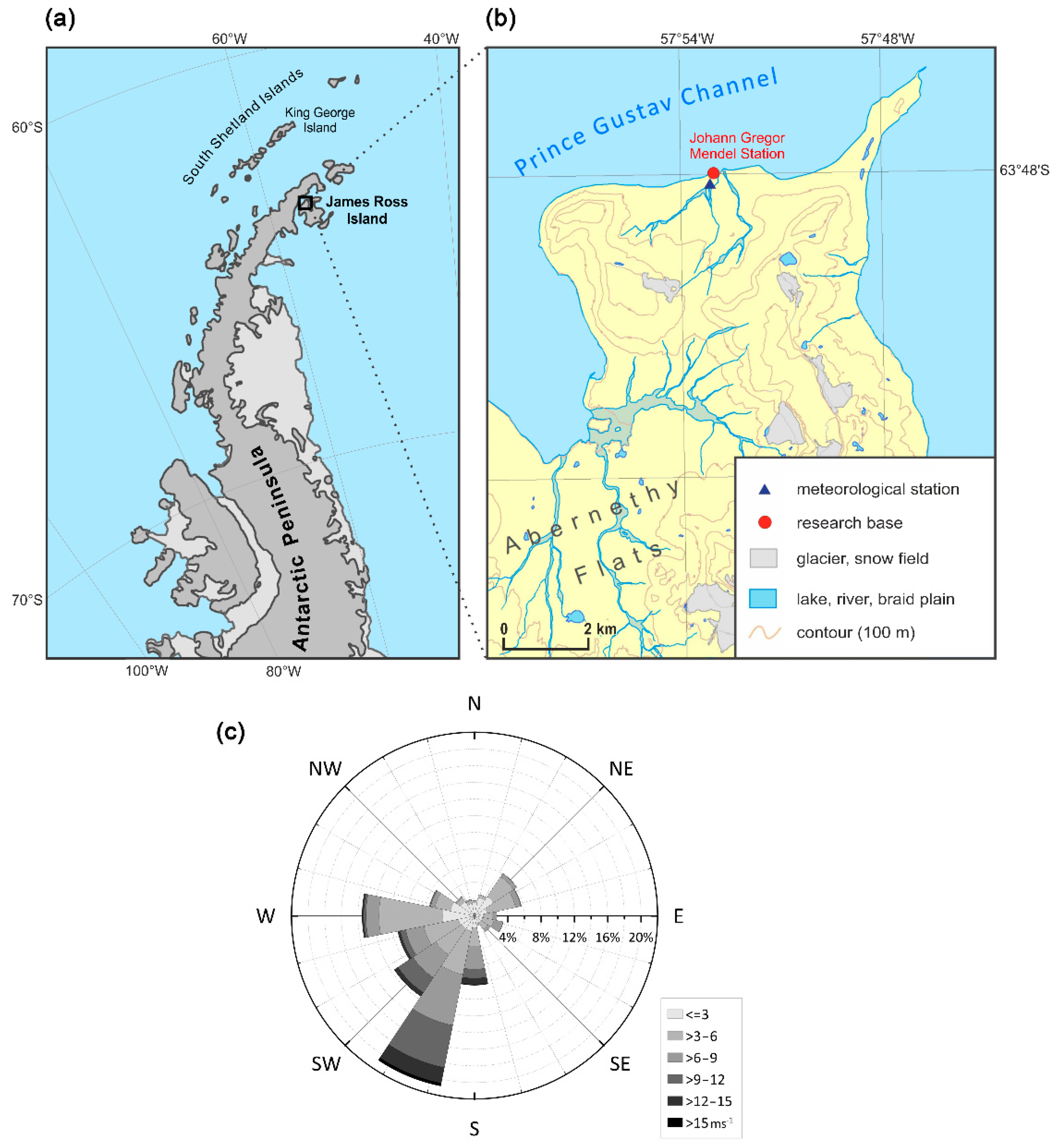
2.1. Study Site and Instrumentation

The Ulu Peninsula, covering 552 km² (see [26]), is the largest ice-free area in the AP region. JRI lies to the south-east of the tip of the AP (Figure 1a), with a prevailing easterly flow often modified by the AP orography in relation to the southern and south-western winds [27]. Consequently, the local climate on JRI is characterized by a 4–5 °C lower mean air temperature compared to the north-western AP [28]. The study site was situated at 10 meters above sea level (m a.s.l.) on a Holocene marine terrace in the northern part of the Ulu Peninsula (Figure 1). The Johann Gregor Mendel Station is located approximately 100 m to the north-east of the meteorological tower and a sonic anemometer, while the seashore is about 150 m to the north. The area is composed of dry sandy ground (about 10% moisture) underlain by continuous permafrost with an active layer of thickness between 50 and 65 cm [23].

The measurements were carried out between 23 January and 21 March, 2018 (58 days). Details on the instruments used for measurements are in

Table 1. Overview of meteorological parameters (“Parameter“) measured on James Ross Island during 23 January–20 March, 2018. In the “Height/Depth“ column, positive numbers refer to height above the ground, while negative numbers refer to depth.

Parameter	Instrument	Company	Height/Depth (m)	Accuracy	Measuring Interval	Recording Interval
Net radiation	CNR4 Net Radiometer	Kipp Zonen, the Netherlands	1	Longwave radiation: ±10%, Shortwave radiation: ±4%	10 s	5 min
Wind components	USA-1 Sonic Anemometer	Metek, Germany	2	0.1 ms−1 or 2%	10 s−1	5 min
Ground heat flux	HFP01 heat flux plates	Huksefluks, the Netherlands	−0.05	±20%	30 min	30 min
Air temperature	EMS33H Sensor	EMS Brno, Czech Republic	2	±0.15 °C	10 s	5 min
Relative humidity	EMS33H Sensor	EMS Brno, Czech Republic	2	±1%	10 s	5 min
Atmospheric pressure	TMAG	CRESSTO, Czech Republic	1	±2 Pa	10 s	5 min
Snow depth	Ultrasonic snow depth sensor	Judd Comm., USA	1	± 1 cm	2 h	2 h
Ground surface temperature	PT100/8 resistance thermometer	EMS Brno, Czech Republic	−0.02, −0.05, −0.10, −0.20, −0.50, −0.75	±0.15 °C	30 min	30 min

and they were all temporarily installed at one site. For the latent heat flux calculation [29], we used the measurements of 2-m air temperature, relative humidity and surface ground temperature measurements. As only relative humidity was measured, 2-m specific humidity was calculated with the use of air temperature and atmospheric pressure data. Furthermore, vertical kinematic eddy heat flux, Monin–Obukhov length and virtual temperature from sonic anemometer were also included in the latent heat flux calculation. The ground surface temperature was defined as the ground temperature at a depth of 2 cm.

2.2. Data Processing and Analysis

The surface energy budget of an ice-free surface can be written as:

$${\mathrm{Q}}_{\mathrm{net}}={\mathrm{Q}}_{\mathrm{G}}+{\mathrm{Q}}_{\mathrm{H}}+{\mathrm{Q}}_{\mathrm{E}}+\mathrm{C}$$

(1)

where Q_net is the net radiation, Q_G is the ground heat flux, Q_H is the sensible heat flux, Q_E is the latent heat flux and C is the residual. The Q_net has the following components:

$${\mathrm{Q}}_{\mathrm{net}}={\mathrm{Q}}_{\mathrm{Snet}}+{\mathrm{Q}}_{\mathrm{Lnet}}={\mathrm{Q}}_{\mathrm{S}\downarrow }+{\mathrm{Q}}_{\mathrm{S}\uparrow }+{\mathrm{Q}}_{\mathrm{L}\downarrow }+{\mathrm{Q}}_{\mathrm{L}\uparrow }$$

(2)

where Q_Snet is the net shortwave flux consisting of incoming (Q_S↓) and outgoing (Q_S↑) shortwave radiation, while Q_Lnet is the net longwave flux, which can be divided into incoming (Q_L↓) and outgoing (Q_L↑) longwave radiation.

All of the measured data were processed as 30-min averages. The Q_S↓ measurements were further corrected with the use of a more precise CM11 pyranometer (Kipp and Zonen). Simple linear regression was used for adding the relative deviation to CNR4 measurement [30]. Surface albedo was calculated daily as the ratio of Q_S↑ and Q_S↓ in the 3 h closest to the maximum of Q_S↓ in order to avoid measurement unreliability under large solar zenith angles and low flux magnitudes.

Ground heat flux measurement was corrected using the calorimetric method [31,32] as follows:

$${\mathrm{G}}_{\mathrm{i}-1}={\mathsf{\delta }\mathrm{z}}_{\mathrm{i}}{\mathrm{C}}_{\mathrm{i}}\left(\frac{\partial {\mathrm{T}}_{\mathrm{i}}}{\partial \mathrm{t}}\right)+{\mathrm{G}}_{\mathrm{i}}$$

(3)

where G_i–1 is the heat flux density at the top of a layer, here at a depth of 2 cm, δz_i is the layer thickness (3 cm), C_i is the volumetric heat capacity for the layer (1.17 MJ m⁻³ K⁻¹ defined for the area by Hrbáček et al. [23]), ∂T_i/∂t is the rate of a 30-min change in the mean layer temperature and G_i is the heat flux density at the bottom of the layer at a depth of 5 cm.

The sensible heat flux was calculated from sonic anemometer using the eddy covariance technique (e.g., [33]). However, it needs to be noted that when the term “sensible heat flux” is used in this study, it is the buoyancy flux, which was calculated instead of true sensible heat flux due to the absence of fast-response moisture measurements [34]. Sensible heat fluxes of 30-min average were calculated only if more than 54% of the measurement were available. Consequently, <2% of sensible heat flux data were missing. Latent heat was calculated as in Langer et al. [29]. Briefly, latent heat flux was estimated as:

$${\mathrm{Q}}_{\mathrm{E}}=-\frac{{\mathsf{\varrho }}_{\mathrm{air}}{\mathrm{L}}_{\lg }}{{\mathrm{r}}_{\mathrm{a}}}\left(\overline{\mathrm{q}}\left({\mathrm{z}}_{\mathrm{m}}\right)-\overline{\mathrm{q}}\left({\mathrm{z}}_0\right)\right)$$

(4)

where ρ_air is the density of air, L_lg is the latent heat of vaporization of water, r_a is atmospheric resistance, q is specific humidity, z_m is measurement height and z₀ is roughness length. Roughness length was originally chosen to be 10⁻³ m over bare ground and 10⁻⁴ m over a snow-covered surface [35,36], but due to unrealistically high values of latent heat flux, they were both lowered by one order to 10⁻⁴ and 10⁻⁵ m, respectively. The atmospheric resistance r_a was calculated as in formula D4 in Langer et al. 2011 [29]. Specific humidity at the surface q(z₀) was derived from the surface temperature using the Magnus formula [37].

Latent heat flux measurements were only available for 92% of the study period. For all surface energy budget components, daily and weekly means were calculated if <20% were missing, hence the loss of daily mean fluxes on 8 February and 12–14 March, 2018 (Figure 2).

The data were mostly analysed and compared as daily means; 30-min averages were only examined in

Table A1. Mean values and 95% confidence interval of selected meteorological variables on James Ross Island during 23 January to 21 March 2018. Shortcuts explanation: shortwave downward radiation (Q_S↓), shortwave upward radiation (Q_S↑), longwave downward radiation (Q_L↓), longwave upward radiation (Q_L↑), net radiation (Q_net), albedo, ground heat flux (Q_G), sensible heat flux (Q_H), latent heat flux (Q_E), air temperature (T_air), ground surface temperature (T_surf) and ground temperature at depth of 50 cm (GT₅₀).

QS↓ (Wm−2)	QS↑ (Wm−2)	QL↓ (Wm−2)	QL↑ (Wm−2)	Qnet (Wm−2)	Albedo
182.7 ± 9.3	33.4 ± 2.2	264.4 ± 1.2	311.1 ± 1.1	102.5 ± 7.2	0.25 ± 0.06
QG (Wm−2)	QH (Wm−2)	QE (Wm−2)	Tair (°C)	Tsurf (°C)	GT50 (°C)
0.5 ± 1.1	32.8 ± 2.0	33.2 ± 2.3	−2.5 ± 0.2	0.1 ± 0.2	−0.2 ± 0.0

and day-long case studies in order to determine the influence of snow and cloudiness on the surface energy budget (Section 3.4). For the correlation analysis (Section 3.3), Spearman’s rank correlation coefficient was used due to non-normal distributions of some data. Simple linear regression was employed for calculating regression function in Section 3.3. The following convention was used: the net radiation components were considered positive if energy transport was directed towards the ground surface; the turbulent and ground heat fluxes were denoted as positive if energy transport was directed away from the ground surface.

For the case studies, it was necessary to determine a cloudy and a clear-sky day. We only had three categories: clear sky, cloudy and overcast. Cloudiness was derived from a combination of hemispherical photos and Q_S↓ measurements. We calculated the mean daily ratio of Q_S↓ to extra-terrestrial radiation (simply approximated from solar constant and solar zenith angle) in hourly intervals. We then estimated that if the daily mean ratio was above 0.6, the sky was (mostly) clear. If the ratio was below 0.4, the day was overcast. Ratios between 0.4 and 0.6 meant a cloudy day.

2.3. Measurement Accuracy

The residual term C in our study was 36.1 ± 104.0 W m⁻² (Table A1), indicating that errors prevented surface energy budget closure. Unlike the measurements from KGI, where C was not determined but was contained within Q_H [17] or Q_G [13], we tried to limit the uncertainty by calculating unmeasured Q_E. Non-zero C has been almost unavoidable in surface energy budget studies from polar regions [29,38], even though errors should have been cancelled out unless there was a systematic error. In our case, 35% of Q_net was allocated to neither Q_G nor the turbulent fluxes due to a combination of multiple measurement errors.

Firstly, the measurement accuracy of the CNR4 for longwave radiation of ±10% might have increased the values of Q_net (

Table 2. Probable error of measurement for different fluxes in this study.

Flux	Error (%)	Reason	Reference
QL↓ (Qnet)	10	Measurement accuracy for longwave radiation	CNR4 Net Radiometer manual
Qnet	3.4	Spatial heterogeneity of albedo around the measuring site	[38]
QH	25	Local circulation systems formation due to complex orography	[39,41]
QH	10	Use of buoyancy flux instead of true sensible heat flux	[34]
QE	33	Choice of z0 (see comment in the text)	Sensitivity testing
QG	20	Measurement accuracy of the instrument	HFP01 heat flux plate manual
QH, QE, QG	-	Different footprint area	[40]

). Moreover, Westermann et al. [38] pointed out that uncertainty about albedo under conditions with patches of snow and bare-ground could be up to 0.1, which would further lower or raise Q_net by 3.4%.

Secondly, the eddy covariance technique requires stationarity. However, complex orography around the measuring site was prone to the development of local circulation patterns [36]. That could have led to systematic underestimation of Q_H up to 25% [39], while the use of buoyancy flux as Q_H means that another 10% might need to be added to Q_H [34].

The error in Q_E was difficult to assess because no comparable measurements existed. Nevertheless, Q_E calculating depended strongly on the correct choice of z₀. In this study, using the values for snow-covered surfaces and bare ground according to current knowledge [35,36] could lead to an increase of Q_E up to 33%. On the other hand, as both Prosek et al. [17] and Choi et al. [13] reported mean Q_E ~ Q_H, it is likely that the error is smaller. Even though the maximum uncertainty in Q_G estimation caused by instrument accuracy could have been up to ±20%, the mean value of Q_G was below 1 W m⁻². As a result, the error in Q_G would not contribute significantly to C.

Finally, individual energy budget components were measured on different spatial scales. Q_G was derived from a point measurement and radiation sensors had a footprint area of several square meters. For the sonic anemometer at a height of 2 m, 60% of the flux might have come from an area with a radius of 75 m or larger [40]. During high wind speeds, the turbulent eddies (and derived energy fluxes) measured by the sonic anemometer were coming from the Bohemian Stream Catchment (see Figure 1 and Section 3.1), where the ground was waterlogged or moister than close to the meteorological tower. Consequently, more energy was allocated to Q_E in the area from which the turbulence was coming, influencing the residual term C.

Considering the above-mentioned errors, the magnitude of C could be explained by the uncertainty inherited from methods of measurements, the landscape diversity around the measuring site and the choice of parameters in the calculation. Essential for future experiment concept and better accuracy of eddy-covariance method could be two-level humidity measurement or krypton hygrometer for measuring water vapour fluctuations with a high-frequency sampling rate.

3. Results

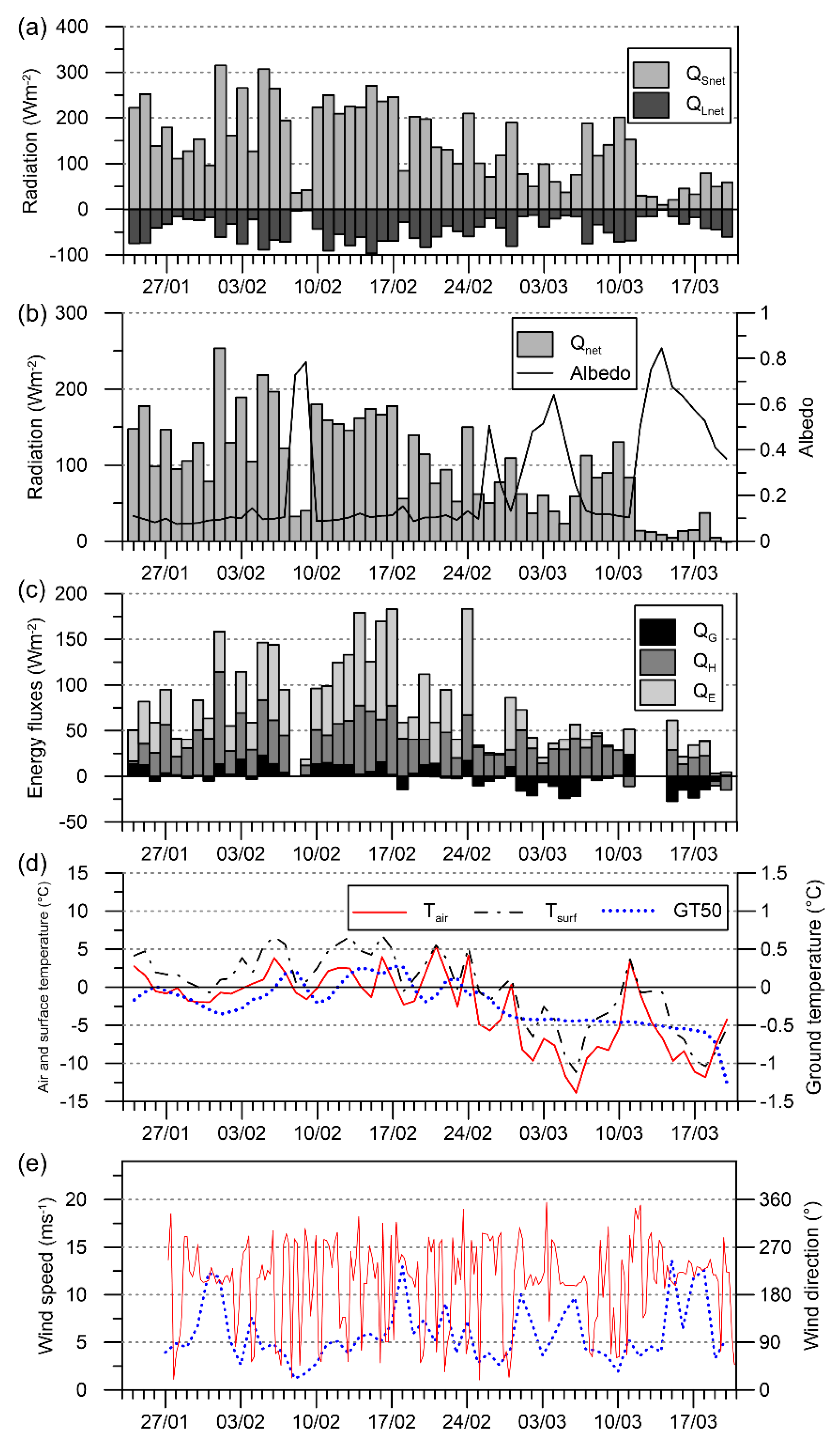
3.1. Meteorological Conditions and Energy Budget Components

From 23 January to 21 March, 2018, the mean daily air temperature on the Ulu Peninsula was −2.5 °C with a range from −13.9 °C to 5.3 °C. Daily mean air temperatures often changed from negative to positive, however, they were <0 °C after 25 February, with the exception of 28 February and 11 March (Figure 2d). On the other hand, the daily mean ground surface temperature was mostly positive before 28 February and mostly negative afterwards. The daily mean ground temperature at 50 cm was −0.2 °C, varying between −1.3 and 0.3 °C only. In 21% of the measurement period, the wind blew from south–southwest (Figure 1c), where the Bohemian Stream catchment lies. The highest mean daily wind speed of 13.6 ms⁻¹ was measured on 15 March, 2018 during south-westerly wind (Figure 2e).

Mean albedo was 0.11 when the ground surface was bare, while it rose to 0.54 on the days with snow cover (Figure 2b). On 8 and 9 February, albedo increased to over 0.70. Snow cover also intensified after 13 March and during 2–5 March, when 3-cm deep snow cover led to the albedo reaching 0.64. The snow cover periods corresponded well to a decrease in mean daily Q_net, which was mostly lower than 40 W m⁻² during the intensified snow cover period and only reached 60 W m⁻² on 3 March.

Mean Q_net was 102.5 W m⁻² and mean Q_L↓ (264.4 W m⁻²) was by 45% higher than mean Q_S↓ (182.7 W m⁻²). Mean Q_L↑ was 311.1 Wm⁻², while mean Q_S↑ was 33.4 Wm⁻² (Table A1). The highest energy budget component, apart from the radiation fluxes, was Q_E with a mean value of 33.2 W m⁻², closely followed by Q_H (32.8 W m⁻²). In both cases, standard deviations were about 1.5times the mean value of the flux. The mean Q_G was only 0.5 W m⁻² due to the averaging–out of positive and negative Q_G (Figure 2c). The residual term C reached 36.1 W m⁻² as a mean value for the study period (more information in Table A1 and Figure A1).

Both mean Q_H and Q_E depended on wind direction (Figure 3). Their mean values were the lowest when the wind was from the east and south-south-east (146.5° to 168.5°), while they were the highest for north-easterly and west-north-westerly wind (281.5° to 303.5°). When the wind was westerly, both mean Q_H and Q_E increased with increasing wind speed (data not shown). Mean Q_H was by 11.1 Wm⁻² higher than mean Q_E for the south–south-westerly wind direction (191.5° to 213.5°), while it was lower for easterly wind (Q_H: 2.5 Wm⁻², Q_E: 13.4 Wm⁻²) and for west–south-westerly to north-west-northerly wind (236.5° to 348.5°, the difference between mean Q_H and mean Q_E of up to 19.6 Wm⁻²). The 95% confidence intervals for both Q_H and Q_E were the lowest for south–south-westerly wind direction (191.5° to 213.5°) and the highest for northerly and north–north-westerly wind direction for Q_H and Q_E, respectively. It is, therefore, clear that in cases of low wind velocity (wind from the northerly sector), higher uncertainty on the closure of surface energy budget occurred and caused higher variation of both turbulent fluxes in the related wind directions.

3.2. Ground Temperature Response to the Largest Surface Energy Fluxes

The ground thermal regime was significantly influenced by individual components of the surface energy budget. Mean daily Q_E was higher than Q_H in 63% of the study period (Figure 2). The highest mean daily Q_H was 100.1 W m⁻² on 1 February (Figure 2). Between 31 January and 1 February, the daily mean ground surface temperature increased by 1.7 °C. Mean daily Q_E was the highest on 24 February (116.2 W m⁻²), when Q_H reached only 50.3 Wm⁻². A concurrent increase in air and ground surface temperature before 24 February pointed to active layer thawing (Figure 4). Between 24 and 25 February, the ground surface temperature decreased by −5.8 °C, indicating that intense evaporation might have led to energy depletion in ground surface layers, which resulted in the drop in surface temperature.

Daily mean Q_G was the highest on 11 March, when it reached 23.9 W m⁻². The Q_G on 11 March led to warming of the whole column from the ground surface to a depth of about 30 cm (Figure 4), with daily mean ground surface temperatures rising by 5.3 °C between 10 and 11 March, while the increase was by 0.2 °C at a depth of 30 cm. On 1 February, 24 February and 11 March, the change in daily mean ground temperature at a depth of 50 cm was never by more than 0.1 °C day⁻¹, even though between 1 and 4 February there was a gradual increase of ground temperature at a depth of 50 cm observed.

Active layer refreezing at the end of the thawing season occurred during 26–28 February (Figure 4). It is clear from Figure 2 that, from 25 to 27 February, daily mean values of Q_G were negative, resulting in a mean heat loss of −5.9 W m⁻². Such a negative mean three-day value of Q_G had not been seen since the start of the measurement. It was also connected to the lowest three-day value of Q_net since 23 January.

3.3. Longer-Term Influence of Surface Energy Budget Components on Ground Temperature Variation

Relationships between ground temperatures and surface energy budget components were the strongest for ground surface temperature and decreased with depth (

Table 3. Daily average correlation coefficients between ground surface temperatures (T_surf), ground temperatures at depth of 30 cm (GT₃₀), 50 cm (GT₅₀) and 75 cm (GT₇₅) and net radiation (Q_net), ground heat flux (Q_G) and air temperature (T_air) on James Ross Island during 23 January to 21 March 2018. The labels “0–3 days“ correspond to the lag of ground temperature time series.

Variable 1	Variable 2	0 Day	1 Day	2 Days	3 Days
Qnet vs.	Tsurf	0.71	0.66	0.64	0.59
	GT30	0.52	0.70	0.71	0.68
	GT50	0.48	0.64	0.67	0.64
	GT75	−0.15	−0.08	−0.01	0.01
QG vs.	Tsurf	0.84	0.72	0.58	0.54
	GT30	0.38	0.59	0.66	0.65
	GT50	0.34	0.44	0.58	0.60
	GT75	−0.01	−0.02	−0.02	0.05
Tair vs.	Tsurf	0.95	0.79	0.63	0.61
	GT30	0.66	0.77	0.77	0.71
	GT50	0.60	0.65	0.72	0.70
	GT75	−0.01	−0.01	0.02	0.11

). For Q_net, the highest correlation coefficients were 0.71 for ground surface temperature and ground temperature at a depth of 30 cm. For Q_G, the difference between the strength of correlations with ground surface temperature and ground temperature at 30 cm was nearly 0.2. For both Q_net and Q_G, correlation coefficients were the highest without a lag for ground surface temperature. Correlation coefficients were close to zero for a depth of 75 cm, which was connected to a nearly isothermal temperature regime with no daily and seasonal variation.

Daily mean Q_G also had several significant and strong relationships with other fluxes (

Table 4. Daily averages correlation matrix of shortwave downward radiation (Q_S↓), shortwave upward radiation (Q_S↑), longwave downward radiation (Q_L↓), longwave upward radiation (Q_L↑), net radiation (Q_net), albedo, ground heat flux (Q_G), sensible heat flux (Q_H), latent heat flux (Q_E), sum of fluxes (Q_G+Q_H+Q_E) and air temperature (T_air). Coefficients in bold are statistically significant on significance level of 0.05. Study site and investigation period are the same as in Table 1.

	QS↓	QS↑	QL↓	QL↑	Qnet	Albedo	QG	QH	QE	QG + QH+ QE	Tair
QS↓	1.00	−0.04	−0.19	0.72	0.91	−0.50	0.78	0.44	0.64	0.76	0.62
QS↑	−0.04	1.00	−0.28	−0.41	−0.33	0.76	−0.20	−0.19	−0.16	−0.30	−0.34
QL↓	−0.19	−0.28	1.00	0.30	0.02	−0.15	0.02	0.20	0.20	0.24	0.34
QL↑	0.72	−0.41	0.30	1.00	0.79	−0.65	0.85	0.34	0.81	0.83	0.96
Qnet	0.91	−0.33	0.02	0.79	1.00	−0.71	0.76	0.60	0.72	0.87	0.67
albedo	−0.50	0.76	−0.15	−0.65	−0.71	1.00	−0.54	−0.29	−0.41	−0.56	−0.53
QG	0.78	−0.20	0.02	0.85	0.76	−0.54	1.00	0.22	0.67	0.72	0.84
QH	0.44	−0.19	0.20	0.34	0.60	−0.29	0.22	1.00	0.50	0.71	0.18
QE	0.64	−0.16	0.20	0.81	0.72	−0.41	0.67	0.50	1.00	0.91	0.78
QG + QH + QE	0.76	−0.30	0.24	0.83	0.87	−0.56	0.72	0.71	0.91	1.00	0.75
Tair	0.62	−0.34	0.34	0.96	0.67	−0.53	0.84	0.18	0.78	0.75	1.00

). For instance, a significant anticorrelation between Q_G and albedo meant that snow cover led to more negative Q_G, hence the flux from deeper levels towards the ground surface. Furthermore, there was a strong positive relationship between Q_G and air temperature. Daily mean Q_G could be expressed by the following regression functions:

$${\mathrm{Q}}_{\mathrm{G}}=5.7+2.1{\mathrm{T}}_{\mathrm{air}}$$

(5)

and

$${\mathrm{Q}}_{\mathrm{G}}=-0.1+2.1{\mathrm{T}}_{\mathrm{surf}}$$

(6)

respectively.

Consequently, an increase in the summer air temperature of 1 °C would lead to an increase in summer Q_G on JRI by 2.1 W m⁻². The relationship between air temperature and ground surface temperature was even stronger than the relationship between air temperature and Q_G, as the correlation coefficient reached 0.95 (Table 3). The reason is that they both primarily respond to Q_net. Consistent with Fourier [42], the lag between Q_G and ground temperature increased with depth. The correlations were quite high probably due to lack of vegetation cover and dry soil, enabling fast heat transport between air and the ground.

3.4. Impact of Snow Cover and Cloudiness

The impact of snow cover and cloudiness was studied with the use of day-long case studies representing contrasting situations that occurred during the summer season. On 4 March (Figure 5b), lower-than-average Q_L↑ (−284.4 W m⁻²) connected to low surface temperature (−2.7 °C) compensated for losses due to reflection from snow cover. Q_L↓ was, for most of the time, 0–5 W m⁻² higher compared with the average daily cycle (Figure 5a) due to the cloudy sky. Q_net was below average apart from a short period between 1300 and 1400 local time when Q_S↓ increased to 940 W m⁻² because of a sudden reduction in cloud cover. Daily mean Q_G on 4 March was −12.7 W m⁻², compared with the mean value of 0.4 W m⁻² (Table 1). The decrease between 4 and 5 March was −4.1 °C day⁻¹ for air temperature and −4.9 °C day⁻¹ for ground surface temperature (Figure 4). Consequently, both the surface and deeper ground levels were losing heat, despite the isolating effect of snow.

The effect of cloudiness was studied on 18 and 15 February, when albedo <0.1 confirmed snow–free conditions. On the overcast day (18 February, Figure 6a), Q_L↓ was, for most of the time, 10–25 W m⁻² higher compared with the average daily cycle (Figure 5a). Daily mean Q_net was 44.8 W m⁻² lower than on the averaged day. Q_G responded to cloudiness by negative values apart from an increase to 10.5 W m⁻² around 1400. Consequently, the mean heat loss of the ground on 18 February was only −11.3 W m⁻², causing a drop of 2.4 °C in daily mean ground temperature at 10 cm depth (Figure 4). On the other hand, on 15 February, the sky was mostly clear apart from one episode of clouds evidenced by sudden decreases in Q_S↓ at 1000 (Figure 6b). The large value of Q_S↓ led to greater daily amplitudes of both Q_net and Q_G with daily means of 171.8 W m⁻² and 6.4 W m⁻², respectively. The supply of heat to the ground was reflected in ground temperature increases between 15 and 16 February from the surface down to 20 cm depth (Figure 4). A sudden increase in Q_E at 1430 was connected to an increase of air temperature above 0°C (Figure 6b).

4. Discussion

4.1. Surface Energy Budget Components in Polar Regions

The values of Q_net, Q_H, Q_E and Q_G from extant surface energy budget studies were only compared for February (Southern Hemisphere) and August (Northern Hemisphere) due to different lengths of measurement periods (Figure 7). Q_net on northern JRI for this month was 46–54% higher than on KGI [13] or dry tundra on Svalbard [43] or Axel Heiberg Island in northern Canada [44]. The only exception was the study from KGI by Prosek et al. [17] where Q_net was only about 10% lower than on JRI. This can be attributed to higher cloudiness on the western side of the AP and a consequent decrease in Q_S↓, as can be evidenced by a lower ratio of Q_net to Q_S↓ in this study (0.56) than in the study from KGI (0.62) by Choi et al. [13].

The value of Q_G on JRI was also slightly higher than on KGI [17], however, in both cases, Q_G comprised about 5% of Q_net on average. The amount of Q_G received by the soil decreases during summer in the ice-free polar regions (e.g., [13,24,29,38]), for instance by −0.46 W m⁻² per 10 days on KGI [17]. Therefore, it is possible that around summer solstice, the soil on JRI might have received up to 5 W m⁻². The ratio of Q_G to Q_net on JRI was 2–4 times lower than in dry Arctic tundra, where summer Q_G usually formed 10–20% of Q_net (e.g., [23,45,46]), which could have been connected to differences in ground surface properties such as vegetation cover and polar day occurrence. In Choi et al. [13], Q_G formed nearly 40% of Q_net on KGI, but the value was most likely overestimated, as it also contained the residual term.

Both on JRI and KGI [17] in February, Q_H was comparable to Q_E. Similar to dry Arctic tundra in late summer, Q_H on JRI also formed about 30% of Q_net (e.g., [44,47]). Summer Q_E in the Arctic were higher than Q_H by 20% to 100% [40] with the difference increasing as the autumn approached (Table 4 in [24,48]). That also seemed to be the case on JRI, as February mean Q_E was about 20% higher than Q_H.

Mean Q_E was higher than Q_H (Figure 3) when the wind was from the westerly sector, while it was vice versa for the south–south-westerly wind. For the westerly sector, there was a clear influence of fetch from the Prince Gustav Channel, which was often free of sea ice. For the south–south-westerly wind, it is likely that measured Q_E would be higher than calculated Q_E, as the ground is waterlogged in that direction (Figure 1).

4.2. Surface Energy Budget Impact on Ground Thermal Regime

The main heat source for ground warming on JRI was Q_net and Q_S↓, as evidenced by the co-occurrence of the most intensive ground warming with the largest Q_net (Figure 2 and Figure 4). For the most part, Q_net supplied heat to Q_G, both turbulent fluxes and ground warming. However, in 53% of the time, the ground was also contributing via Q_G to warming the air, which also occasionally happened in the dry Arctic (western Greenland) [45]. On 11 March, Q_net and Q_H were the main energy sources, as the ground was cooler than the air above (Figure 2). On that day, the available energy was penetrating well via the frozen ground due to higher thermal conductivity of frozen compared to unfrozen ground, which led to slight ground warming (Figure 4). From the surface energy budget components, the closest relationship of ground temperature was found to be with Q_G.

The energy transfer via the ground was similar on the eastern and western sides of the AP, as demonstrated, for instance, by the correlations between Q_net and ground temperatures on JRI (this study) and KGI [17]. At the measurement site on northern JRI, there was bare ground, while Prosek et al. [17] carried out measurements over regularly flooded ground covered with a 3-cm-thick vegetation cover consisting of 30% moss and 70% grass. It is, therefore, clear that the insulating effect of vegetation cover acted to delay the energy transfer, which might have consequently operated at the level of days rather than hours.

The specific climate conditions and the absence of vegetation cover on JRI study site strongly influenced the ground thermal regime, as the ground temperature at a depth of 10 cm was about 4 °C lower than for the corresponding period in Arctic lichen tundra (Figure 7 in [49]). The ground without vegetation on JRI cooled more during the night, when the ground temperature at a depth of 10 cm fell to −0.4 °C, compared with a minimum of 2.3 °C in the Arctic.

The ground thawed and froze frequently both on JRI and KGI [17], but while Prosek et al. [17] observed refreezing of the whole active layer profile on KGI within 9 days, on JRI it was only 3 days.

4.3. Snow Cover and Cloudiness Effects

On JRI, the insulating effect of snow on Q_G and the ground thermal regime was considered as rather negligible, both in this study and by Hrbacek et al. [50]. However, the maximum snow height reached only 26 cm during 23 January to 20 March, 2018 on JRI. Langer et al. [29] noticed that, at the Lena River Delta, the insulating effect was the most pronounced during winter, while, later in the year, the heat stored in the soil was depleted, meaning that snow insulation was of minor relevance. Furthermore, the high albedo of snow prevented the ground from receiving Q_S↓ [44], which would have reduced ground cooling.

The radiation paradox [51] was not observed on JRI, as the effect of cloudiness was to cool the ground surface and soil layer, since the decrease in Q_S↓ was not compensated for by an increase in Q_L↓. Such conditions also occurred in summer on Svalbard [52]. For individual days, the difference in Q_net and Q_G, due to lower cloudiness on JRI, could have been up to 120 and 17.5 W m⁻², respectively, while the difference in Q_net was only 100 W m⁻² across the tundra in Svalbard [43]. The cloud cover is usually less dense on the eastern side of the AP, as is documented, for instance, by the difference of 32 W m⁻² in Q_L↓ between this study and Hurd Peninsula glaciers on Livingston Island [14]. That could mean a significant increase in Q_net and Q_G on JRI with respect to the western side of the AP.

Neither the snow nor cloudiness affected Q_H in summer significantly, both on the eastern and western sides of the AP [13]. One reason might have been that Q_H responses to wind speed, as was shown earlier (Figure 3), and air-surface temperature differences, which do not always have to be connected to cloud cover development. Unlike on KGI [13], less energy was partitioned to Q_E on the day with snow than on the day with extensive cloud cover.

5. Conclusions

In this study, the surface energy budget and its impact on the ground thermal regime were studied on JRI during January–March 2018. The main findings were:

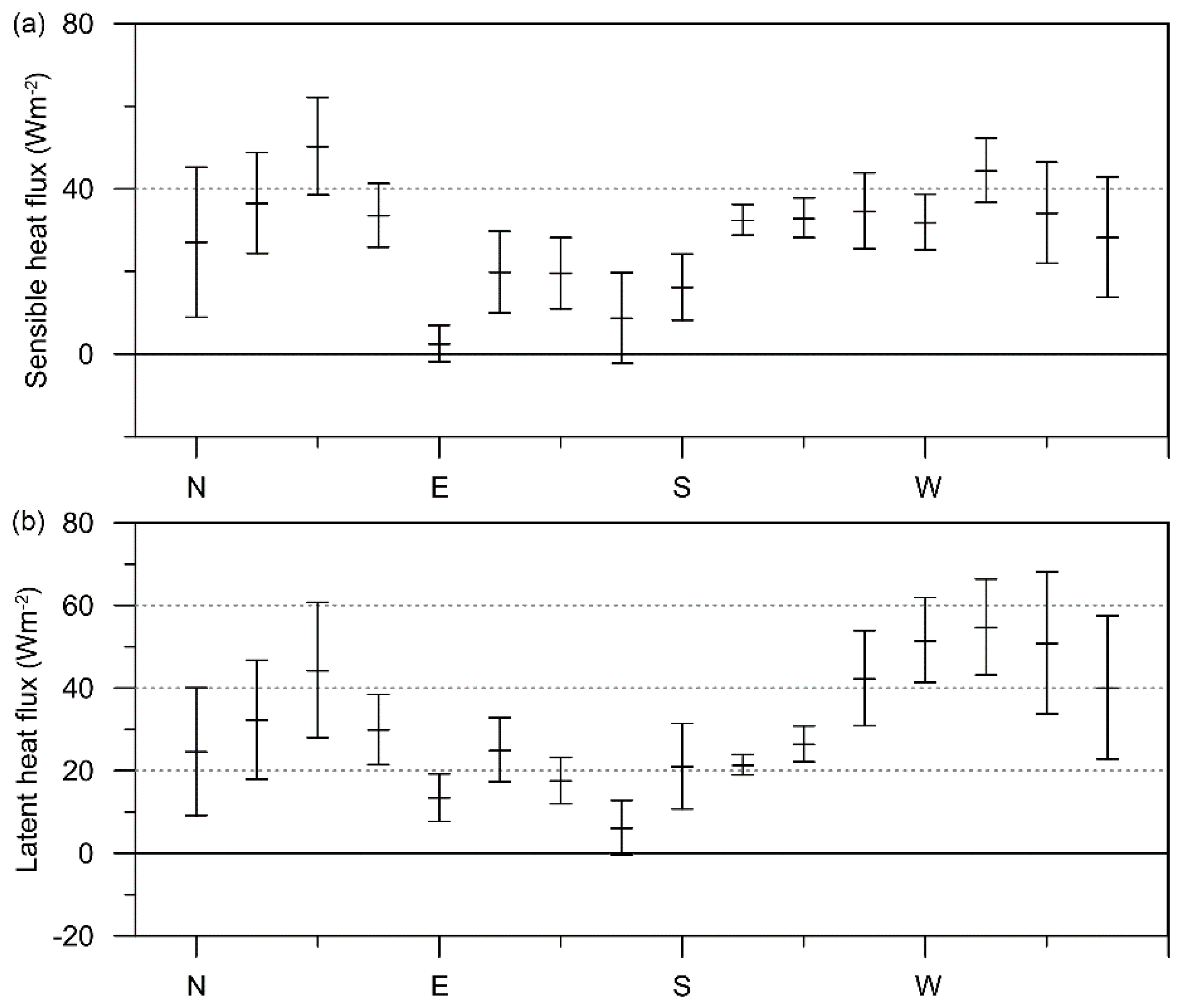
• Mean Q_net reached 102.5 W m⁻², while the highest mean daily Q_net was 253 W m⁻². Mean Q_G was only 0.5 W m⁻² and yet 46% of the time the ground was a heat source for the atmosphere. Mean Q_E was only by 0.4 Wm⁻² higher than mean Q_H. Mean Q_E was up to 19.6 W m⁻² higher than mean Q_H when the wind blew from west–south-westerly to north–west-northerly sector (236.5° to 348.5°), showing the influence of increased moisture availability from the sea.
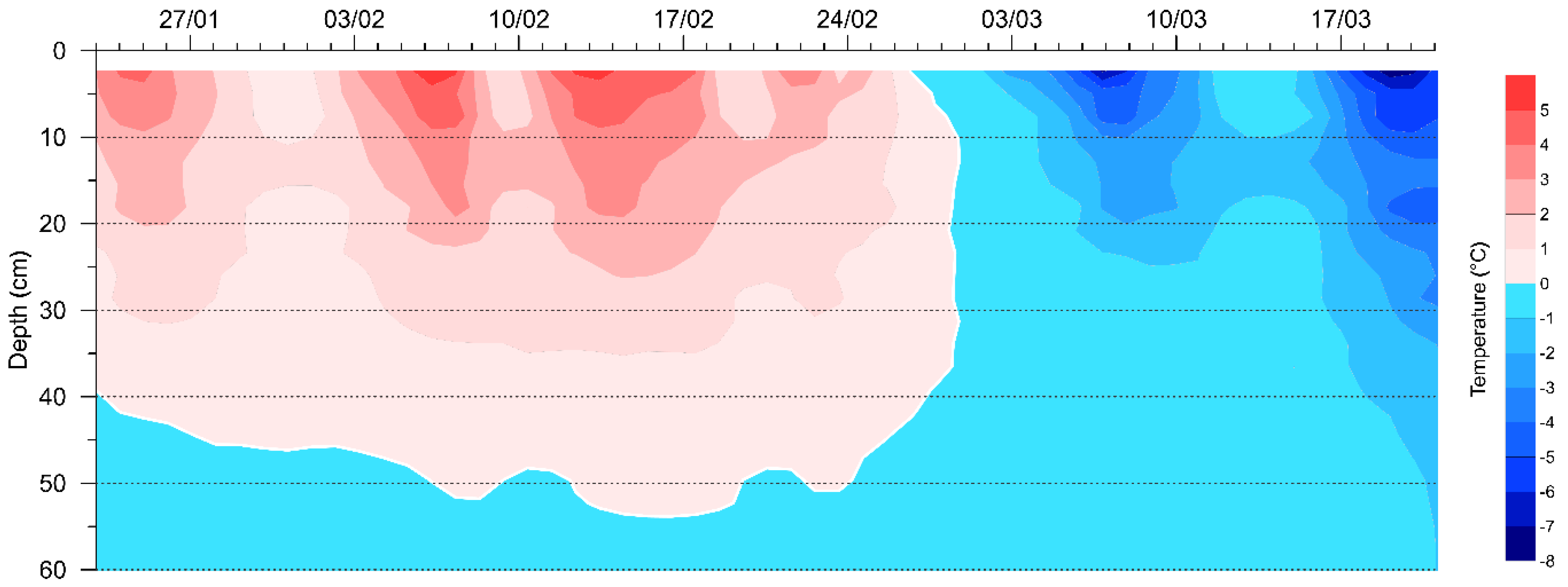
• The ground thermal regime was affected by surface energy budget components to the depth of 50 cm. The strongest relationship was found between Q_G and the ground surface temperature, with a delay growing along with increasing depth. The active layer refroze at the end of February after a sequence of three days with continuously negative Q_G.
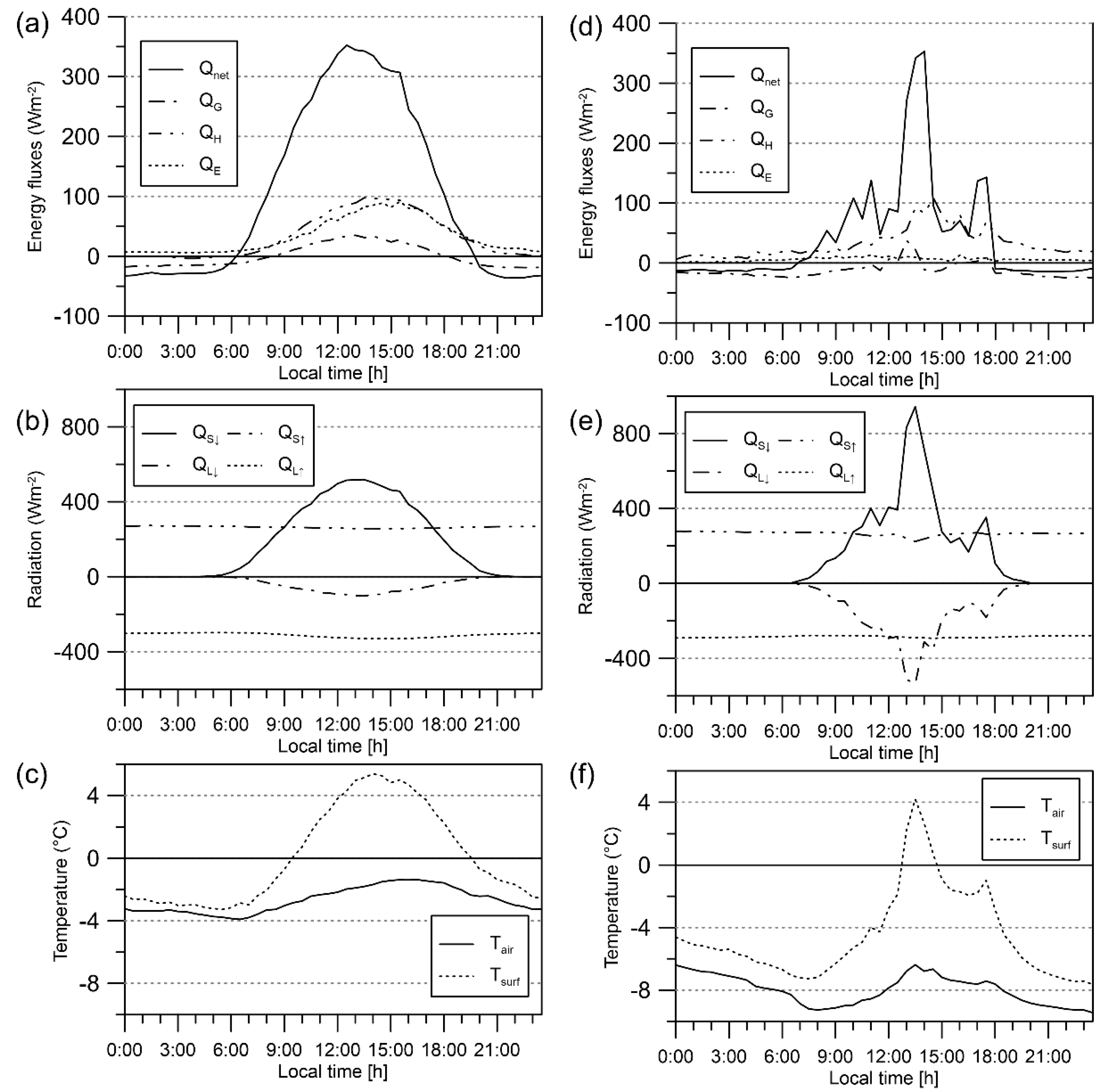
• The case studies have shown that an increase of cloud cover led to a decrease of both mean daily Q_net and Q_G which caused cooling in ground thermal profile. On a clear-sky day, the situation was vice versa.
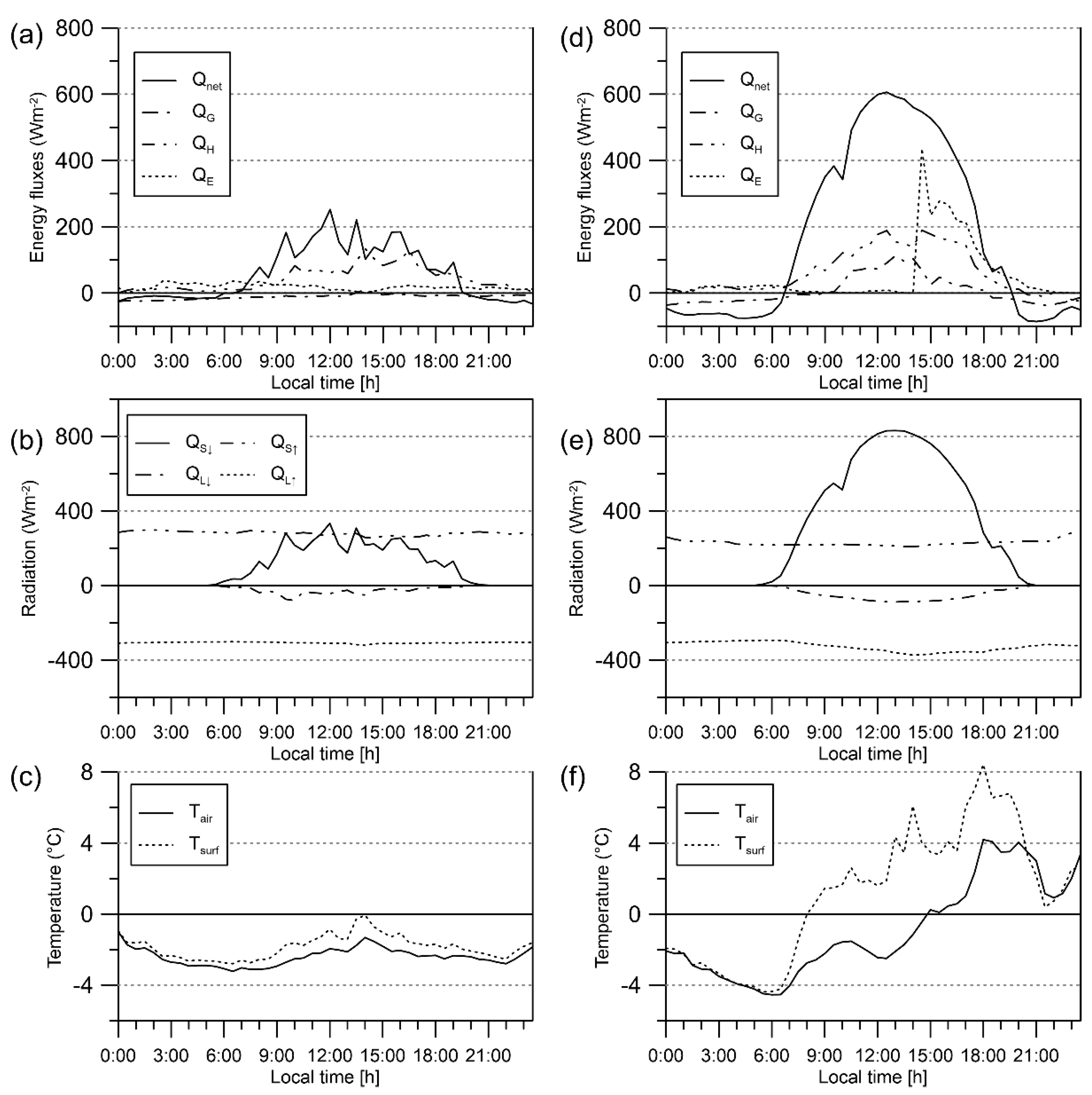
• Insulation by snow cover was not observed, as Q_G was 13.2 W m⁻² below average and the ground was cooling in the whole profile during a sample day with snow cover.
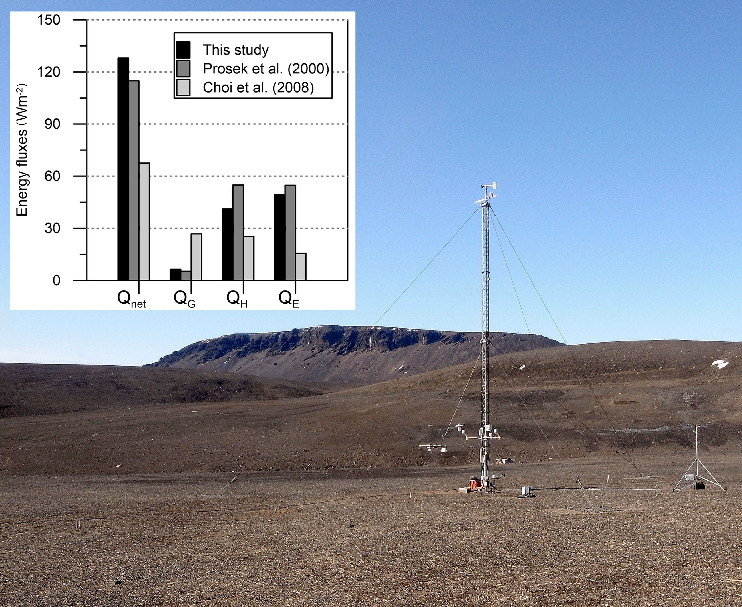
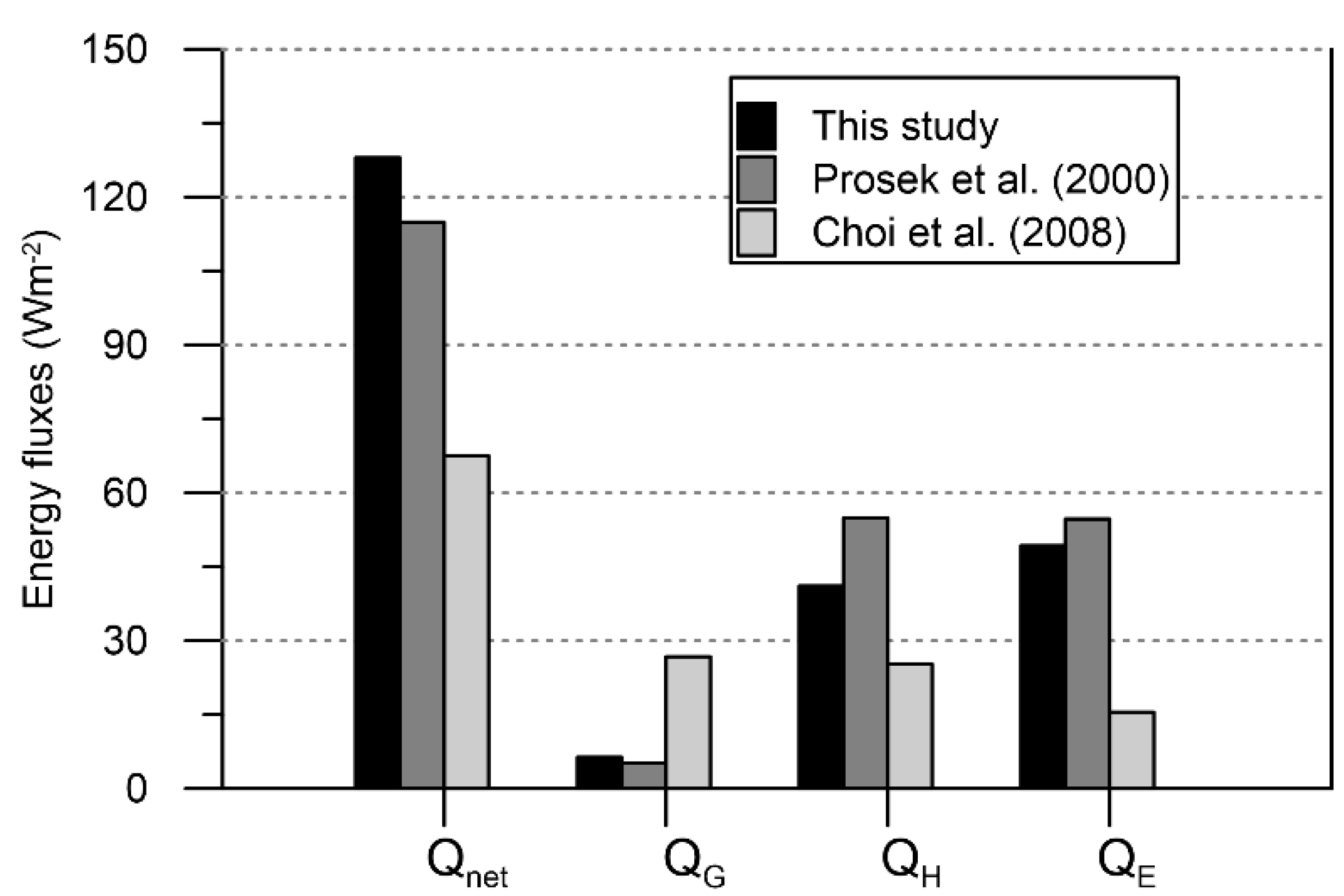
• By comparison with other studies, we concluded that Q_net was higher on the eastern side of the AP due to less cloudiness affected by regional atmospheric patterns. Mean Q_G reached similar values on the eastern and western side of the AP and comprised about 5% of Q_net, approximately four-times less than was observed in the Arctic summer months. Mean Q_E was, on both sides of the AP, approximately the same as Q_H, even though the ratio of Q_H to Q_net varied by 15% among the studies.

Summer energy fluxes (Q_H and Q_E) are crucial for the AP glaciers due to warming effect and efficient snow and ice melting (e.g., [9,14]), although they were mostly heat sources for the atmosphere in our study site. Ice-free areas might, accordingly, be an important source of energy in the AP region and should be considered in regional climate models. As all the surface energy budget studies from ice-free regions in Antarctica so far have only been seasonal, a deeper understanding of the surface energy budget would be gained from a full-year data set. The reported climate evolution of the AP region is currently slightly uncertain [8]. Should the warming observed since the 1950s continue, existing ice-free areas are more likely to be enlarged. Consequently, a study of the interannual and spatial variability in the surface energy budget in ice-free areas in Antarctica would provide valuable new information about how these new environments might influence the land-atmosphere interactions and the future climate of Antarctica.

The data that support the findings of this study are available from the corresponding author upon reasonable request.

References

1. King, J.C.; Turner, J. Antarctic Meteorology and Climatology; Cambridge University Press: Cambridge, UK, 1997; pp. 1–425. [Google Scholar]
2. Burton-Johnson, A.; Black, M.; Fretwell, P.T.; Kaluza-Gilbert, J. An automated methodology for differentiating rock from snow, clouds and sea in Antarctica from Landsat 8 imagery: A new rock outcrop map and area estimation for the entire Antarctic continent. Cryosphere 2016, 10, 1665–1677. [Google Scholar] [CrossRef] [Green Version]
3. Fox, A.J.; Cooper, A.P.R. Climate-change indicators from archival aerial photography of the Antarctic Peninsula. Ann. Glaciol. 1998, 27, 636–642. [Google Scholar] [CrossRef] [Green Version]
4. ATCM. Antarctic Trial of WWF’s Rapid Assessment of Circum-Arctic Ecosystem Resilience (RACER) Conservation Planning Tool: Results of RACER Workshop Focused on James Ross Island. Information paper by Great Britain and Czechia. In Proceedings of the 38th Antarctic Treaty Consultative Meeting, Sofia, Bulgaria, 14 December 2015. [Google Scholar]
5. Lee, J.R.; Raymond, B.; Bracegirdle TJChadès, I.; Fuller, R.A.; Shaw, J.D.; Terauds, A. Climate change drives expansion of Antarctic ice-free habitat. Nature 2017, 547, 49–54. [Google Scholar] [CrossRef] [PubMed]
6. Turner, J.; Lu, H.; White, I.; King, J.C.; Phillips, T.; Hosking, J.S.; Bracegirdle, T.J.; Marshall, G.J.; Mulvaney, R.; Deb, P. Absence of 21st century warming on Antarctic Peninsula consistent with natural variability. Nature 2016, 535, 411–415. [Google Scholar] [CrossRef] [Green Version]
7. Oliva, M.; Navarro, F.; Hrbacek, F.; Hernández, A.; Nývlt, D.; Pereira, P.; Ruiz-Fernández, J.; Trigo, R. Recent regional climate cooling on the Antarctic Peninsula and associated impacts on the cryosphere. Sci. Total Environ. 2017, 580, 210–223. [Google Scholar] [CrossRef]
8. Gonzalez, S.; Fortuny, D. How robust are the temperature trends on the Antarctic Peninsula? Antarct. Sci. 2018, 30, 322–328. [Google Scholar] [CrossRef] [Green Version]
9. Bintanja, R. The local surface energy balance of the Ecology Glacier, King George Island, Antarctica: Measurements and modelling. Antarct. Sci. 1995, 7, 315–325. [Google Scholar] [CrossRef]
10. Braun, M.; Saurer, H.; Vogt, S.; Simões, J.C.; Goßmann, H. The Influence of Large-Scale Atmospheric Circulation on the Surface Energy Balance of the King George Island Ice Cap. Int. J. Climatol. 2001, 21, 21–36. [Google Scholar] [CrossRef]
11. King, J.C.; Argentini, S.A.; Anderson, P.S. Contrasts between the summertime surface energy balance and boundary layer structure at Dome C and Halley stations, Antarctica. J. Geophys. Res. 2006, 11, D02105. [Google Scholar] [CrossRef]
12. Vihma, T.; Johansson, M.M.; Launiainen, J. Radiative and turbulent surface heat fluxes over sea ice in the western Weddell Sea in early summer. J. Geophys. Res. 2009, 114, C04019. [Google Scholar] [CrossRef] [Green Version]
13. Choi, T.; Lee, B.Y.; Kim, S.-J.; Yoon, Y.J.; Lee, H.-C. Net radiation and turbulent energy exchanges over a non-glaciated coastal area on King George Island during four summer seasons. Antarct. Sci. 2008, 20, 99–111. [Google Scholar] [CrossRef] [Green Version]
14. Jonsell, U.Y.; Navarro, F.J.; Bañón, M.; Lapazaran, J.J.; Otero, J. Sensitivity of a distributed temperature-radiation index melt model based on AWS observations and surface energy balance fluxes, Hurd Peninsula glaciers, Livingston Island, Antarctica. Cryosphere 2012, 6, 539–552. [Google Scholar] [CrossRef] [Green Version]
15. Alves, M.; Soares, J. Diurnal Variation of Soil Heat Flux at an Antarctic Local Area during Warmer Months. Appl. Environ. Soil. Sci. 2016, 2016, 9. [Google Scholar] [CrossRef] [Green Version]
16. Perrson, P.O.G.; Stone, R.S.; Grachev, A.; Matrosova, L. Processes Affecting the Annual Surface Energy Budget at High-Latitude Terrestrial Sites. In Proceedings of the EGU Conference, Vienna, Austria, 22–27 April 2012. [Google Scholar]
17. Prosek, P.; Janouch, M.; Láska, K. Components of the energy balance of the ground surface and their effect of the thermics of the substrata of the vegetation oasis at Henryk Arctowski Station, King George Island, South Shetland Islands. Polar Rec. 2000, 36, 3–18. [Google Scholar] [CrossRef]
18. Foken, T. The Energy Balance Problem: An Overview. Ecol. Appl. 2008, 18, 1351–1367. [Google Scholar] [CrossRef]
19. Lunardini, V.J. Heat Transfer in Cold Climates; Van Nostrand-Reinhold: New York, NY, USA, 1981; pp. 1–731. [Google Scholar]
20. Roth, K.; Boike, J. Quantifying the thermal dynamics of a permafrost site near Ny-Ålesund, Svalbard. Water Resour. Res. 2001, 37, 2901–2914. [Google Scholar] [CrossRef]
21. Williams, P.J.; Smith, M.W. The Frozen Earth: Fundamentals of Geocryology; Cambridge University Press: Cambridge, UK, 1989; pp. 1–306. [Google Scholar]
22. Ling, F.; Zhang, T. A numerical model for surface energy balance and thermal regime of the active layer and permafrost containing unfrozen water. Cold Reg. Sci. Technol. 2004, 38, 1–15. [Google Scholar] [CrossRef]
23. Hrbáček, F.; Kňažková, M.; Nývlt, D.; Láska, K.; Mueller, C.W.; Ondruch, J. Active layer monitoring at CALM-S site near J. G. Mendel Station, James Ross Island, eastern Antarctic Peninsula. Sci. Total Environ. 2017, 601–602, 987–997. [Google Scholar] [CrossRef] [PubMed]
24. Eugster, W.; Rouse, W.R.; Pielke, R.A.; Mcfadden, J.P.; Baldocchi, D.D.; Kittel, T.G.; Chapin, I.I.I.F.S.; Liston, G.E.; Vidale, P.L.; Vaganov, E.; et al. Land-atmosphere energy exchange in Arctic tundra and boreal forest: Available data and feedbacks to climate. Glob. Chang. Biol. 2000, 6, 84–114. [Google Scholar] [CrossRef]
25. Van Wessem, J.M.; Reijmer, C.H.; Van de Berg, W.J.; van Den Broeke, M.R.; Cook, A.J.; van Ulft, L.H.; van Meijgaard, E. Temperature and wind climate of the Antarctic Peninsula as simulated by a high-resolution regional atmospheric climate mode. J. Clim. 2015, 28, 7306–7326. [Google Scholar] [CrossRef] [Green Version]
26. Kavan, J.; Ondruch, J.; Nývlt, D.; Hrbáček, F.; Carrivick, J.L.; Láska, K. Seasonal hydrological and suspended sediment transport dynamics in proglacial streams, James Ross Island, Antarctica. Geogr. Ann. A 2017, 99, 38–55. [Google Scholar] [CrossRef]
27. Bohuslavová, O.; Macek, P.; Redčenko, O.; Láska, K.; Nedbalová, L.; Elster, J. Dispersal of lichens along a successional gradient after deglaciation of volcanic mesas on northern James Ross Island, Antarctic Peninsula. Polar Biol. 2018, 41, 2221–2232. [Google Scholar] [CrossRef]
28. Hrbáček, F.; Oliva, M.; Láska, K.; Ruiz-Fernández, J.; De Pablo, M.A.; Vieira, G.; Ramos, M.; Nývlt, D. Active layer thermal regime in two climatically contrasted sites of the Antarctic Peninsula region [Régimen termal de la capa activa en dos áreas climáticamente. contrastadas de la Península Antártica]. Cuad. Investig. Geogr. 2016, 42, 457–474. [Google Scholar]
29. Langer, M.; Westermann, S.; Muster, S.; Piel, K.; Boike, J. The surface energy balance of a polygonal tundra site in northern Siberia—Part 1: Spring to fall. Cryosphere 2011, 5, 151–171. [Google Scholar] [CrossRef] [Green Version]
30. Wilks, D. Statistical Methods in the Atmospheric Sciences; Academic Press: Cambridge, MA, USA, 2011; pp. 1–704. [Google Scholar]
31. Fuchs, M. Heat flux. In Methods of Soil Analysis. Part I. Physical and Mineralogical Methods, 2nd ed.; Klute, A., Ed.; SSSA Book Series no. 5; SSSA: Madison, WI, USA, 1986; pp. 957–968. [Google Scholar]
32. Sauer, T.J.; Horton, R. Micrometeorology in Agricultural Systems. Agronomy Monograph no. 47; American Society of Agronomy, Crop Science Society of America; Soil Science Society of America: Madison, WI, USA, 2005; pp. 1–154. [Google Scholar]
33. Foken, T. Micrometeorology; Springer: Berlin/Heidelberg, Germany, 2008; pp. 1–1306. [Google Scholar]
34. Liu, H.; Foken, T. A modified Bowen ratio method to determine sensible and latent heat fluxes. Meteorol. Z. 2001, 10, 71–80. [Google Scholar] [CrossRef]
35. Gromke, C.; Manes, C.; Walter, B.; Lehning, M.; Guala, M. Aerodynamic Roughness Length of Fresh Snow. Bound-Layer Meteorol. 2011, 141, 21–34. [Google Scholar] [CrossRef] [Green Version]
36. Liu, C.; Li, Y.; Yang, Q.; Wang, L.; Wang, X.; Li, S.; Gao, Z. On the surface fluxes characteristics and roughness lengths at Zhongshan station, Antarctica. Int. J. Digit. Earth 2019, 12, 878–892. [Google Scholar] [CrossRef]
37. Harrison, R.G. Meteorological Measurements and Instrumentation; Wiley Blackwell: Chichester, UK, 2015; pp. 1–257. [Google Scholar]
38. Westermann, S.; Lüers, J.; Langer, M.; Piel, K.; Boike, J. The annual surface energy budget of a high-arctic permafrost site on Svalbard, Norway. Cryosphere 2009, 3, 245–263. [Google Scholar] [CrossRef] [Green Version]
39. Ambrozova, K.; Laska, K.; Hrbacek, F.; Kavan, J.; Ondruch, J. Air temperature and lapse rate variation in the ice-free and glaciated areas of northern James Ross Island, Antarctic Peninsula, during 2013–2016. Int. J. Climatol. 2019, 39, 643–657. [Google Scholar] [CrossRef]
40. Wilson, K.; Goldstein, A.; Falge, E.; Aubinet, M.; Baldocchi, D.; Berbigier, P.; Bernhofer, C.; Ceulemans, R.; Dolman, H.; Field, C.; et al. Energy balance closure at FLUXNET sites. Agric. Meteorol. 2002, 113, 223–243. [Google Scholar] [CrossRef] [Green Version]
41. Burba, G.; Anderson, D. A Brief Practical Guide to Eddy Covariance Flux Measurements: Principles and Workflow Examples for Scientific and Industrial Applications; LI-COR Biosciences: Lincoln, NE, USA, 2010; 212p. [Google Scholar]
42. Fourier, J. The Analytical Theory of Heat; Dover Publications: New York, NY, USA, 1955; pp. 1–66. [Google Scholar]
43. Kejna, M.; Przybylak, R.; Araźny, A. The Influence of Cloudiness and Synoptic Situations on the Solar Radiation Balance in the Area of Kaffiøyra (NW Spitsbergen) in the Summer Seasons 2010 and 2011. Bull. Geogr. Phys. Geogr. Ser. 2012, 5, 77–95. [Google Scholar] [CrossRef] [Green Version]
44. Ohmura, A. Comparative Energy Balance Study for Arctic Tundra, Sea Surface, Glaciers and Boreal Forests. Geojournal 1984, 8, 221–228. [Google Scholar] [CrossRef]
45. Rott, H.; Obleitner, F. The Energy Balance of Dry Tundra in West Greenland. Arct. Alp. Res. 1992, 24, 352–362. [Google Scholar] [CrossRef]
46. Harding, R.J.; Lloyd, C.R. Fluxes of water and energy from high latitude tundra sites in Svalbard. Nord. Hydrol. 1998, 29, 267–284. [Google Scholar] [CrossRef]
47. Scherrer, D.; Parlow, E.; Ritter, N.; Siegrist, F. Klimaoökologie und Fernerkundung. In Methoden und Datenübersicht der Forschungsgruppen der Geowissenschaftlichen Spitzbergen-Expeditionen 1990 und 1991 zum Liefdefjorden (Datenband) Materialien zur Physiogeographie; Leser, H., Ed.; Geographisches Institut: Basel, Switzerland, 1993; Volume 15, pp. 51–58; appendix 121–151. [Google Scholar]
48. Sjøblom, A. Turbulent fluxes of momentum and heat over land in the High-Arctic summer: The influence of observation techniques. Polar Res. 2014, 33, 1–17. [Google Scholar] [CrossRef] [Green Version]
49. Migała, K.; Wojtuń, B.; Szymański, W.; Muskała, P. Soil moisture and temperature variation under different types of tundra vegetation during the growing season: A case study from the Fuglebekken catchment, SW Spitsbergen. Catena 2014, 116, 10–18. [Google Scholar] [CrossRef]
50. Hrbáček, F.; Láska, K.; Engel, Z. Effect of Snow Cover on the Active-Layer Thermal Regime–A Case Study from James Ross Island, Antarctic Peninsula. Permafr. Periglac. Process. 2016, 27, 307–315. [Google Scholar] [CrossRef]
51. Ambach, W. The Influence of Cloudiness on the Net Radiation Balance of a Snow Surface with High Albedo. J. Glaciol. 1974, 13, 73–84. [Google Scholar] [CrossRef] [Green Version]
52. Kejna, M.; Maturilli, M.; Araźny, A.; Sobota, I. Radiation balance diversity on NW Spitsbergen in 2010–2014. Pol. Polar Res. 2017, 39, 61–82. [Google Scholar] [CrossRef]
Figure 1. Antarctic Peninsula (AP) region (a), measuring site on Ulu Peninsula, James Ross Island (b) and wind rose representing wind frequencies with respect to their wind speed from study site for period from 23 January to 21 March, 2018 (c).
Atmosphere 11 00877 g001
Figure 2. Daily averages of (a) net shortwave radiation (QSnet), net longwave radiation (QLnet), (b) net radiation (Qnet) and albedo, (c) ground heat flux (QG), sensible heat flux (QH) and latent heat flux (QE), (d) air temperature (Tair), ground surface temperature (Tsurf) and ground temperature at depth of 50 cm (GT50), (e) wind speed (WS) and wind direction (as six-hourly immediate values, WD). Note that latent heat flux was calculated.
Atmosphere 11 00877 g002
Figure 3. Mean and 95% confidence interval of sensible heat flux (a) and latent heat flux (b) depending on wind direction at study site between 23 January and 21 March 2018.
Atmosphere 11 00877 g003
Figure 4. Ground temperature development at study site between 23 January and 21 March 2018.
Atmosphere 11 00877 g004
Figure 5. Daily regimes of surface energy budget components on James Ross Island between 23 January and 21 March 2018: averaged day (left column) and day with snow cover (right column, 4 March). (a,d): net radiation (Qnet), ground heat flux (QG), sensible heat flux (QH) and latent heat flux (QE). (b,e): incoming shortwave radiation (QS↓), outgoing shortwave radiation (QS↑), incoming longwave radiation (QL↓) and outgoing longwave radiation (QL↑). (c,f): air temperature (Tair) and ground surface temperature (Tsurf).
Atmosphere 11 00877 g005
Figure 6. Daily regimes of surface energy budget components: day with overcast sky (left column, 18 February) and day with clear sky (right column, 15 February. (a,d): net radiation (Qnet), ground heat flux (QG), sensible heat flux (QH) and latent heat flux (QE). (b,e): incoming shortwave radiation (QS↓), outgoing shortwave radiation (QS↑), incoming longwave radiation (QL↓) and outgoing longwave radiation (QL↑). (c,f): air temperature (Tair) and ground surface temperature (Tsurf).
Atmosphere 11 00877 g006
Figure 7. February mean net radiation (Qnet), ground heat flux (QG), sensible heat flux (QH) and latent heat flux (QE) on James Ross Island (this study) and King George Island according to studies by Prosek et al. [17] and Choi et al. [13].
Atmosphere 11 00877 g007